Orbital and freshwater forcing during the last interglacial: analysis of climate and vegetation response patterns

(1)

HAL Id: hal-00298162

https://hal.archives-ouvertes.fr/hal-00298162

Submitted on 5 Dec 2006

HAL is a multi-disciplinary open access

archive for the deposit and dissemination of sci-entific research documents, whether they are pub-lished or not. The documents may come from teaching and research institutions in France or abroad, or from public or private research centers.

L’archive ouverte pluridisciplinaire HAL, est destinée au dépôt et à la diffusion de documents scientifiques de niveau recherche, publiés ou non, émanant des établissements d’enseignement et de recherche français ou étrangers, des laboratoires publics ou privés.

Orbital and freshwater forcing during the last

interglacial: analysis of climate and vegetation response

patterns

G. Lohmann

To cite this version:

G. Lohmann. Orbital and freshwater forcing during the last interglacial: analysis of climate and vegetation response patterns. Climate of the Past Discussions, European Geosciences Union (EGU), 2006, 2 (6), pp.1221-1247. �hal-00298162�

(2)

CPD

2, 1221–1247, 2006 Orbital and freshwater forcing: climate and vegetation patterns G. Lohmann Title Page Abstract Introduction Conclusions References Tables Figures ◭ ◮ ◭ ◮ Back Close

Full Screen / Esc

Printer-friendly Version Interactive Discussion

Clim. Past Discuss., 2, 1221–1247, 2006 www.clim-past-discuss.net/2/1221/2006/ © Author(s) 2006. This work is licensed under a Creative Commons License.

Climate of the Past Discussions

Climate of the Past Discussions is the access reviewed discussion forum of Climate of the Past

Orbital and freshwater forcing during the

last interglacial: analysis of climate and

vegetation response patterns

G. Lohmann

Alfred Wegener Institute for Polar and Marine Research, Bremerhaven, Germany

Received: 20 November 2006 – Accepted: 26 November 2006 – Published: 5 December 2006 Correspondence to: G. Lohmann ([email protected])

(3)

CPD

Full Screen / Esc

Abstract

Large-scale atmospheric patterns are examined on orbital timescales using the ECHO-G which explicitly resolves the atmosphere – ocean – sea ice dynamics. It is shown that in contrast to boreal summer where the climate mainly follows the local radiative forcing, the boreal winter climate is strongly determined by modulation of the atmo-5

spheric circulation. We find that during a positive phase of the Arctic Oscillation/North Atlantic Oscillation the convection in the tropical Pacific is below normal. The atmo-spheric circulation patterns induce non-uniform temperature anomalies, much stronger in amplitude than by the direct solar insolation. Together with the direct solar insola-tion this provides for a temperature drop over the Northern Hemisphere continents for 10

115 000 years before present, large areas over northern Asia and Alaska become a desert, and the grass land expanded to the north. The spatial pattern of temperature and vegetation changes differs from a more hemisphere-wide cooling, i.e. induced by oceanic freshwater in the northern North Atlantic. The signatures of different forcing mechanisms are important for the interpretation of proxy data as well as for the under-15

standing of underlying mechanisms at the end of the last interglacial.

1 Introduction

Various terrestrial and marine records show that the Holocene and the last interglacial were marked by coherent patterns of climate variability at a regional or global scale. Pollen-based temperature reconstructions suggest a temperature drop from 120 to 20

115 ky BP (ky BP: 1000 years before present) in northern and central Europe for boreal winter and summer (K ¨uhl and Litt, 2003). Coral data from the northern Red Sea sug-gest a modulation of the seasonal cycle for the Eemian and late Holocene climate (Felis et al., 2004). These patterns of past climate variability are often related to changes in major phenomena that dominated the climate variability during the last century, like the 25

(4)

Ki-CPD

Full Screen / Esc

toh and Murakami, 2002) or the Arctic Oscillation/North Atlantic Oscillation (AO/NAO) (Keigwin and Pickart, 1999; Rimbu et al., 2003, 2004; Lorenz et al., 2006).

Recently, Sirocko et al. (2005) presented evidence for multi-centennial cooling events in the central European continent, and suggested a possible weakening of the oceanic meridional overturning circulation during this time interval. Such cooling may be anal-5

ogous to the 8.2 kyr BP event, both in the mechanism and duration. The 8.2 kyr BP event was the most prominent climatic event occurring in the early Holocene (Alley et al., 1997), and is evident in numerous proxy records. A salinity anomaly in the North Atlantic caused by the outflow of two Laurentide glacial lakes is thought to be a trig-ger for the event, transferring its effects globally (Renssen et al., 2001). Such events 10

induce global environmental responses, at least in the Northern Hemisphere, but the magnitude, spatial expression and mechanisms are not well understood. Global cli-mate proxy records will be collated in the future and compared to assess the varying nature of recorded environmental changes. Here, we show different climate patterns in order to understand Related global teleconnections and mechanisms will enlarge our 15

understanding of climate variations during interglacials.

The spatial heterogeneity of interglacial climate evolution is examined by applying general circulation models and addressing the modulation of large-scale climate modes on orbital time scales. We concentrate on the dynamic evolution of the Northern Hemi-sphere atmospheric circulation during the past 140 000 years with special emphasis on 20

the last interglacial temperature evolution, making use of coupled atmosphere-ocean-sea ice general circulation models.

2 Methodology

2.1 Orbital forcing

The Earth’s orbital parameters are the eccentricity of the Earth’s orbit, the angle be-25

tween the vernal equinox and the perihelion on the orbit, and the obliquity (Milankovitch, 1223

(5)

CPD

Full Screen / Esc

1941). The calculation follows Berger (1978) providing the incoming solar radiation at the top-of-atmosphere as a function of latitude and time.

Figure 1shows the changing solar irradiance due to the slowly evolving orbital pa-rameters from 140 ky BP until 100 ky BP at the boreal summer and winter, respec-tively. The insolation achieves its maximum between 130 and 125 ky BP and around 5

105 ky BP at Northern Hemisphere summer solstice. This is due to both, a larger tilt of the Earth’s rotation axis and the precession cycle, moving the passage of the Earth through its perihelion from boreal summer in the early Eemian to the beginning of January today. In the Eemian and early Holocene the insolation achieved a strong deviation from today’s values. This is due to both a larger tilt of the Earth’s rotation axis 10

and the precession cycle, moving the passage of the Earth through the perihelion from boreal summer in the last interglacial and early Holocene to the beginning of January today. At the winter solstice, a lack of insolation during the last interglacial is strongest at about 127 ky BP and is centered around the equator. This is due to the precession cycle, since the distance to the Sun is then at its maximum in boreal winter. The large 15

excentricity during the Eemian provides for a large difference between the Holocene and Eemian conditions for the stregth of the precessional cycle.

2.2 Climate model ECHO-G driven by orbital parameters

For the simulation of interglacial climate changes owing to orbital forcing, we apply the coupled atmosphere-ocean general circulation model ECHO–G (Legutke and Voss, 20

1999). The atmospheric part of this model is the circulation model ECHAM4 (Roeckner et al., 1996) with T30 horizontal resolution (approximately 3.8◦

×3.8◦) and 19 vertical levels. The ECHO-G model has been adapted to account for the influence of the annual distribution of solar radiation due to the slowly varying orbital parameters. The ocean model includes a dynamic-thermodynamic sea-ice model with snow cover and has a 25

resolution of approximately 2.8◦

×2.8◦. The model consists of 20 irregularly spaced vertical levels with 10 levels covering the upper 300 m.

(6)

CPD

Full Screen / Esc

pre-industrial era (280 ppm CO₂, 700 ppb CH₄, and 265 ppb N₂O) and modern irradi-ance. This experiment has been integrated over 3000 years of model simulation into a pre-industrial climate state, which is regarded as the quasi-equilibrium response of the model to pre-industrial boundary conditions. It serves as a baseline and initialization of the simulations.

5

Computer resources for running a complex model like ECHO-G over the time period of the last interglacial and the Holocene are very demanding. Therefore, the time scale of the orbital forcing has been shortened by an acceleration factor of 100, which im-plies that the response of the system to insolation forcing is completed after centuries. In effect, this procedure decouples any slowly responding portions of the system (e.g., 10

deep water properties) from the feedback structure. For our long-term simulations we neglect possible changes in deep-ocean circulation and concentrate on the atmo-spheric dynamics.

In our earlier paper (Lorenz and Lohmann, 2004), we presented arguments that the overturning circulation is only slightly affected through the insolation forcing during the 15

Holocene. With our method, we have excluded effects like that the surface conditions in the Southern Ocean may experience a delayed response to radiative forcing due to the influence of the deep-ocean circulation (Goosse and Renssen, 2001).

The long runs over the last 140 000 years are continued to the next 30 000 years into the future. The last 140 000 years are therefore represented in 1400 model years. For a 20

detailed description we refer to Lorenz and Lohmann (2004) where the effect of the ac-celeration factor is evaluated on Holocene climate trends. It is found that the magnitude of orbitally forced Holocene trends is largely independent of the chosen acceleration factor. Throughout the whole experiments fixed greenhouse gas concentrations (latest Holocene values: 280 ppm CO2, 700 ppb CH4, 265 ppb N2O) and modern values for 25

vegetation, land-ocean and continental ice distribution, and sea level were used. As discussed by Joussaume and Braconnot (1997) a precise comparison of astro-nomical seasons under different orbital parameters would be to define the length of the months on the basis of their current angle on the earth’s orbit. Due to Kepler’s Law,

(7)

CPD

Full Screen / Esc

on the elliptical orbit the track speed is not constant. For example, the respectively defined time interval for the today’s JJA season (1 June to 30 August concerning the model’s year of 360 days) lies for the 130 ky BP time slice from 25 May until 19 August (85 days in 130 ky BP instead of 90 days today). We calculated the new “JJA” and “DJF” surface temperature field for different time slices on this basis and found that the 5

maximum error is less than 1◦_{C with much lower values at low latitudes (not shown).} Therefore, we stick to the simple calculation by using the fixed 90 days for the DJF and JJA seasons in our analysis.

2.3 Global vegetation model LPJ

The Lund-Potsdam-Jena dynamic global vegetation model (LPJ) by Sitch et al. (2003) 10

combines process-based descriptions of the terrestrial ecosystem structure (vegeta-tion composi(vegeta-tion, biomass and height) and func(vegeta-tion (energy absorp(vegeta-tion, carbon cy-cling). Vegetation composition is described by nine different plant functional types (PFT), which are distinguished according to their physiological, morphological (tree, grass) and phenological (deciduous, evergreen) attributes.

15

The model is run on a grid-cell basis with a specified atmospheric CO2concentration and soil texture. Monthly fields of temperature, precipitation and radiation are taken from the output of ECHO-G. Each grid-cell is divided into fractions covered by PFTs and bare ground. Both the presence and the covered fraction of PFTs within a grid-cell depend on their specific environmental limits and on resource competition among the 20

PFTs.

The vegetation dynamics is calculated for the period 140 to 100 ky BP, where mov-ing chunks of 10-years output of the atmospheric GCM are used to create the forcmov-ing, which is necessary to resolve the typical timescale of the vetation dynamics. Prior to the transient run, the vegetation model is run for 3000 years of integration into equilib-25

rium, using 15 years of monthly data from the period 140 ky BP repeatedly as input for the LPJ model.

(8)

CPD

Full Screen / Esc

2.4 ECHAM3/LSG: release of freshwater

In order to analyse the climatic effect of a catastrophic release of freshwater into the Labrador Sea, the coupled atmosphere-ocean circulation model ECHAM3/LSG (Voss et al., 1998) has been employed. The ocean model has a free surface and includes a thermodynamic sea-ice model. The coupled model has a horizontal resolution of about 5

5.6◦

.

In the experiment, a large freshwater anomaly in the northern North Atlantic is re-leased in equal parts to two grid points on the Canadian coast of the Labrador Sea. The experimental setup of this scenario is described elsewhere (Schiller et al., 1997; Lohmann, 2003). The freshwater input to the Labrador Sea forces a transient shutdown 10

of the THC reducing the northward heat transport in the Atlantic Ocean. The circulation recovers completely after about 600 years when the freshwater input was switched off (Schiller et al., 1997). For our analyses, the model output of years 140–150 is taken. At this time, the overturning circulation is at about 50% of its present-day value of 18 Sv (1 Sv=1×106m3s−1₎

.

15

3 Results

3.1 Climate model ECHO-G forced by orbital parameters

Figure 2 displays the temperature evolution of the Northern Hemisphere from 140 ky BP until 30 ky after present under astronomical forcing. The only forcing in the experiment is given by the insolation changes due to earth orbital parameters. The 20

temperature evolution for the boreal summer and winter are dominated by the preces-sional cycle (modulated by eccentricity), and are mainly out of phase. For the boreal summer, a long-term cooling trend for 15 to 0 ky BP is detected. At 3 ky BP, the insola-tion at the top of the atmosphere almost reached the present energy level. In the next millenia, an increase in the boreal summer and a lowered boreal winter insolation is 25

(9)

CPD

Full Screen / Esc

linked to the precessional cycle. For comparison, the red lines in Fig.2show the tem-perature evolution for the the period 1900–2000 AD as evaluated with the same model, but with increased greenhouse gas concentrations (Lorenz and Lohmann, 2004). The model simulations can be interpreted as climate evolution for the interglacial periods, where changes in ice sheets played a minor role compared to the last glacial period. 5

The amplitudes of insolation changes are much larger for the last interglacial, than for the Holocene, because the eccentricity – affecting the precessional cycle – is around 4.1% compared to roughly 1.7% in the Holocene. The changes in the future are go-ing to further decrease, since the eccentricity, followgo-ing its 100 and 400 kyr cycles, decreases nearly to zero during the following 50 kyr (Berger and Loutre, 2002).

10

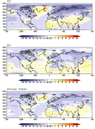
Figure3displays the surface air temperature simulated for boreal winter (December– January–February, DJF), summer (June–July–August, JJA), and annual mean at 115 minus 120 ky BP. In our model, the surface temperature trends, especially during DJF, show pronounced spatial heterogeneity. The Labrador Sea warms up, whereas large parts of Europe tend to cool. The summer warming in the Labrador Sea area is due 15

to the stored winter signal in the oceanic mixed layer. Such an anomaly pattern is detected for weakening of the Icelandic Low. The boreal summer cooling trend is very pronounced which is linked to the insolation forcing (Fig.1a). Figure 4 displays the anomalous sea level pressure (SLP) where the weakening of the Icelandic Low is detected. The weakened westerlies over the northern North Atlantic associated with 20

the AO/NAO in its negative phase (Fig. 4) is associated to the spatial heterogeneity seen in the regional temperatures (Fig.3a). At southern high latitudes, a polar warm-ing is accompanied by reduced westerlies (Fig. 4). The amplitude of the circulation changes are higher for the upper levels in the atmosphere (not shown). Furthermore, a baroclinic relation between SLP and surface air temperature (high DJF pressure and 25

temperatures over the Nordic Seas) shows that the atmospheric circulation is induced by temperature change. The high temperatures in the Nordic Seas would otherwise be associated with a thermodynamically-induced low pressure system in this area.

(10)

in-CPD

Full Screen / Esc

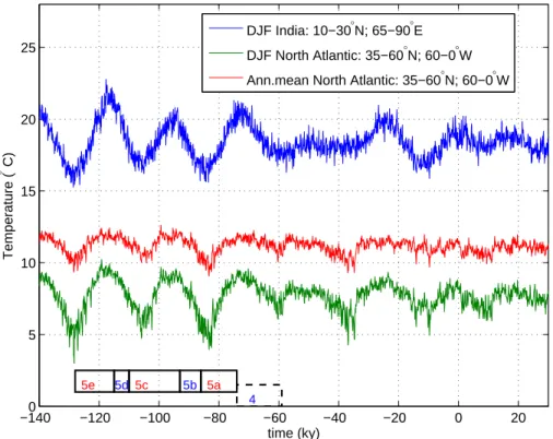
terglacial values for 125 to 115 ky BP for boreal winter and spring (not shown). For 115 ky BP, the winter surface temperature anomaly indicates a tendency toward a low AO/NAO index state, with cold winters in central Europe due to reduced advection of warm oceanic air from the west. The boreal winter circulation changes cannot be explained by local insolation, but with atmospheric circulation anomalies. The time evo-5

lution for the winter Northern Hemisphere temperature indices are displaced in Fig.5. It shows that the annual mean temperature evolution is linked to the boreal winter North Atlantic temperature. The winter signal is out of phase with that of the the boreal sum-mer. The Indian surface temperature is laging the North Atlantic index by 1000 years caused by insolation (Fig.5).

10

3.2 Evolution of the vegetation cover

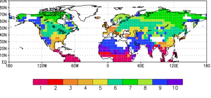
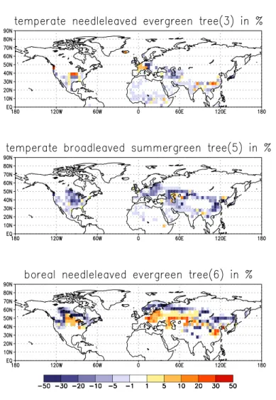
In order to test the sensitivity of the Northern Hemisphere vegetation cover with respect to the different climate conditions, the LPJ dynamical vegetation model is used as a diagnostic tool for the last interglacial climate evolution. The LPJ model calculates, besides other results, the fraction of the PFT with respect to the varying climate of 15

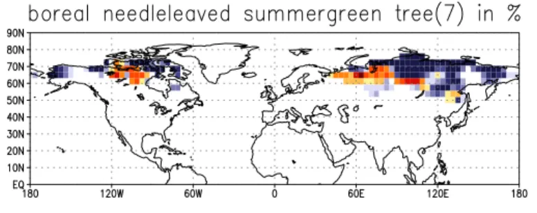
the ECHO-G experiments (Fig.6). The analysis of the vegetation distribution for 120 and 115 ky BP indicates a strong southward shift of the boreal trees. The fraction of boreal needleleaved evergreen trees (Fig.7) and boreal summergreen trees (Fig. 8) decreases by 50%. Large areas over northern Asia and Alaska become a desert (Fig.6), over Scandinavia and parts of North America, the C3 perennial grass becomes 20

the dominant PFT. The tropical PFTs show little variations and are therefore not shown in Figs.7,8.

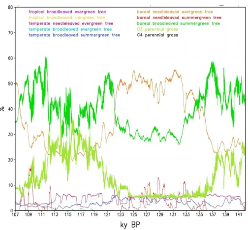
Figure9shows the evolution of the plant functional types over northern Europe (north of 50◦_{N, 0–40}◦_{E). For the period 122 to 132 ky BP, about 50% of Northern Europe was} covered by boreal needleleaved evergreen trees, followed by an abrupt increase of bo-25

real broadleaved summergreen trees. These summergreen trees were partly relaced in the period around 115 ky BP by C3 grass. It is interesting to note that the temperature and precipitation temporal characteristics in this area is smooth.

(11)

CPD

Full Screen / Esc

3.3 Interglacial meltwater pulse

Furthermore, the effect of a freshwater release into the Labrador Sea is shown for in-terglacial background conditions mimicking a perturbation induced by runoff or calving from the North American continent. Caused by the freshwater release to the North Atlantic, the THC slows down to 9 Sv (Lohmann, 2003) and the northern North Atlantic 5

cools considerably (Fig.10) where the strongest cooling is over the Nordic Seas caused by advanced sea-ice cover. The summer cooling is less extended with only half of the temperature response of the winter signal (Fig.10). Figure 11 shows surface winds during the freshwater release for the boreal winter season. We find enhanced south-ward winds in the Greenland Sea, over the Denmark Strait, and south of Greenland 10

favouring the transport of polar water masses into the North Atlantic.

4 Discussion and conclusions

A major factor in the pacing of climate change on time scales of tens of thousands of years, seems to be the change in seasonal sunlight distribution or insolation induced by variations in the Earth’s orbital parameters (e.g., Imbrie et al., 1993; Berger et al., 15

1993). The shape of the Earth’s orbit shifts from more elliptical to more circular at periodicities of about 100 000 years. Other rhythms are linked to the tilt of the Earth’s axis (periodicities of 29 000, 41 000, and 54 000 years), and the timing of the seasons relative to the Earth’s closests position to the Sun on the orbit (periodicities of 19 000 and 23 000 years).

20

For the orbital forcing, an acceleration technique is applied that has enabled us to run the coupled GCM for the equivalent of 140 000 years. With a normal setup of such models, this would not have been feasible due to the considerable computing require-ments of these models. The applied acceleration technique for ECHO-G assumes that the impact of changes in the deep ocean on surface temperatures is small compared 25

(12)

CPD

Full Screen / Esc

The basic assumption in the ECHO-G model setup is that the time scales of the astronomical forcing at the above mentioned frequencies can be separated from the much shorter time scales of the atmosphere-ocean-sea ice system, and that variations of the thermohaline circulation during interglacials played a minor role compared to other periods. These assumptions justify our procedure in the model configuration, 5

where the astronomical forcing is accelerated (Lorenz and Lohmann, 2004).

Here, we concentrate on the effect of orbital forcing on the dynamics during the last interglacial and the glacial inception. We focus on the boreal winter season since it strongly determines the long-term signal in SST. The fact that part of the winter SST signal is seen in the summer anomaly pattern (Fig.3) is due to the rectifying effect of the 10

ocean: Upper-ocean temperature anomalies are preserved over summer and reappear in the following fall and winter. This could have implications for the documentation of the temperature signal in proxies. The winter signal is preserved for long-term climate variability, and the documented signal can be biased toward the winter climate signal, even when not identical with the season when blooming takes place.

15

Furthermore, we find a non-linear response of the vegetation plant functional types over northern Europe (Fig.9). Abrupt shifts in vegetation cover are detected at 115, 122, 132 ky BP. It is conceivable that the vegetation cover reacts in a nonlinear way to smooth climate variations due to thresholds. This finding emphasizes that a proper transfer function is required in order to translate the vegetation signal into a climate 20

signal.

There are evidences for multi-centennial cooling events possibly induced by the oceanic meridional overturning circulation (Sirocko et al., 2005). Here, we compare the seasonal signal of such cooling events with that induced by orbital forcing. In an-other model set-up, we performed freshwater perturbation experiments in the northern 25

North Atlantic for an interglacial background state (Fig.10). Although a direct com-parison with the simulations for the effect of Earth’s orbital parameters is not possible due to another model and model resolution, it can be seen that the sudden freshwater input (Fig.10) has a stronger effect on climate than the gradual Milankovitch forcing for

(13)

CPD

Full Screen / Esc

115 ky BP (cf. Fig.3).

Caused by the freshwater release and cold climate in the North Atlantic, surface winds are affected. We find enhanced southward winds in the Greenland Sea, over the Denmark Strait, and south of Greenland (Fig.11) favouring the transport of polar water masses into the North Atlantic. This may be an analogous situation with the 5

8.2 ky BP event as well as with the Great Salinity Anomaly in the late sixties (Dickson et al., 1988) with a freshwater transport out of the Arctic Ocean. Such freshening event which temporarily interrupted deep water renewal in the Labrador Sea are probably reinforced by southward winds in the Greenland Sea. It can be speculated whether this positive feedback is responsible for long-persisting temperature anomalies in the 10

North Atlantic on multidecadal time scales.

We find that the temperature reduction from 120 to 115 ky BP in northern and central Europe is up to 6◦_{C for boreal winter and up to 3}◦_{C for boreal summer, respectively} (Fig. 3). The effect is strongest where the sea ice cover changed north of Sibiria, a similar amplifying mechanism is also detected for the Holocene (Lohmann et al., 15

2005). The simulated temperature changes are matched by pollen-based temperature reconstructions that reveal an approx. 3◦_{C summer cooling and a 10}◦_{C winter cooling at} the end of the Eemian in central Europe (K ¨uhl and Litt, 2003). The strong winter cooling in the model is due to the change in circulation (Fig. 4) associated to a weakened Icelandic Low.

20

Our finding of the Icelandic Low modulation on orbital time scales is consistent with alkenone-based SST reconstructions for the Holocene (Lorenz et al., 2006). A positive phase of the AO/NAO at 6 ky BP relative to present-day is accompanied by low insola-tion in the tropical region. Furthermore, modelling experiments reveal that changes in the regional circulation in the Nordic Seas during the Holocene is compatible with the 25

Milankovitch forcing (Lohmann et al., 2005). Additional high resolution spatio-temporal proxy data sets are necessary to examine the spatial and temporal patterns of climate variability during the last interglacial.

(14)

CPD

Full Screen / Esc

proxy records indicating mild winters in Europe (Zagwijm, 1996; Aalbersberg and Litt, 1998; Klotz et al., 2003) and associated cold winters in the northern Red Sea (Felis et al., 2004). The astronomically driven circulation in the model is in line with the analysis of the seasonal signal in an atmospheric circulation model (Hall et al., 2005). Consistent with pollen-based temperature reconstructions (K ¨uhl and Litt, 2003), we find 5

a temperature drop from 120 to 115 ky BP in northern and central Europe for boreal winter and summer, respectively. A large part of the strong winter cooling is due to the change in Northern Hemisphere circulation associated to a weakened Icelandic Low. It can be speculated that the glacial inception is due to the direct effect of insolation and atmospheric dynamics, i.e. summer cooling in combination with a negative phase 10

of the AO/NAO during winter. A similar argument may be valid for the MIS5a to 4 transition crossing a potential threshold from the the last interglacial to glacial climate. As a logical next step, future studies should include the interactions of atmospheric dynamics with other climate components such as vegetation and land ice, possibly amplifying the climate response as detected in our simulation.

15

Acknowledgements. Thanks go to S. Schubert, S. Lorenz, and M. Scholze for their support.

Part of this work was supported by the Bundesministerium f ¨ur Bildung und Forschung through DEKLIM, and by the Deutsche Forschungsgemeinschaft through DFG Research Centre Ocean Margins at Bremen University.

References

20

Aalbersberg, G. and Litt, T.: Multiproxy climate reconstructions for the Eemian and Early We-ichselian, J. Quat. Sci., 13, 376–390, 1998.

Alley, R. B., Sowers, T., Mayewski, P. A., Stuiver, M., Taylor, K. C., and Clark, P. U.: Holocene cli-matic instability: A prominent, widespread event 8200 yr ago, Geology, 25, 483–486, 1997. Berger, A. L.: Long-term variations of daily insolation and Quaternary climatic changes, J. 25

Atmos. Sci., 35, 2362–2367, 1978

Berger, A. and Loutre, M.-F.: An exceptionally long interglacial ahead?, Science, 297, 1287– 1288, 2002.

(15)

CPD

Full Screen / Esc

Berger, A., Loutre, M.-F., and Tricot, C.: Insolation and Earth’s Orbital Periods, J. Geophys. Res., 98(D6), 10 341–10 362, 1993.

Clement, A. C., Seager, R., and Cane, M. A.: Orbital controls on ENSO and the tropical climate, Paleoceanography, 14, 441–456, 1999.

Dickson, R. R., Meincke, J., Malmberg, S. A., and Lee, A. J.: The “Great Salinity Anomaly” in 5

the northern Atlantic 1968–1982, Prog. Ocean., 20, 103–151, 1988.

Felis, T., Lohmann, G., Kuhnert, H., Lorenz, S. J., Scholz, D., P ¨atzold, J., Al-Rousan, S. A., and Al-Moghrabi, S. M.: Increased seasonality in Middle East temperatures during the last interglacial period, Nature, 429, 164–168, 2004.

Hall, A., Clement, A., Thompson, D. W. J., Broccoli, A., and Jackson, C.: Atmospheric dynamics 10

govern northern hemisphere wintertime climate variations forced by changes in earth’s orbit, J. Climate, 18, 1315, 2005.

Imbrie, J., Berger, A., Boyle, E. A., Clemens, S. C., Duffy, A., Howard, W. R., Kukla, G., Kutzbach, J., Martinson, D. G., McIntyre, A., Mix, A. C., Molfino, B., Morley, J. J., Peterson, L. C., Pisias, N. G., Prell, W. L., Raymo, M. E., Shackleton, N. J., and Toggweiler, J. R.: On the 15

structure and origin of major glaciation cycles: 2. the 100,000-year cycle, Paleoceanography, 8, 701–738, 1993.

Joussaume, S. and Braconnot, P.: Sensitivity of paleoclimate simulation results to season defi-nitions, J. Geophys. Res., 102(D2), 1943–1956, 1997.

Keigwin, L. D. and Pickart, R. S.: Slope Water Current over the Laurentian Fan on Interannual 20

to Millennial Time Scales, Science, 286, 520–523, 1999.

Klotz, S., Guiot, J., and Mosbrugger, V.: Continental European Eemian and early Wuermian climate evolution: Comparing signals using different quantitative reconstruction approaches based on pollen, Global Planetary Change, 36(4), 277–294, 2003.

K ¨uhl, N. and Litt, T.: Quantitative time series reconstruction of Eemian temperature at three 25

European sites using pollen data, Veget. Hist. Archaeobot., 12, 205–214, 2003.

Legutke, S. and Voss, R.: The Hamburg atmosphere-ocean coupled circulation model ECHO-G, Technical report No. 18, Deutsches Klimarechenzentrum, Hamburg, 1999.

Lohmann, G., Lorenz, S. J., and Prange, M.: Northern high-latitude climate changes dur-ing the Holocene as simulated by circulation models, in: The Nordic Seas: An Integrated 30

Perspective, edited by: Drange, H., Dokken, T., Furevik, T., Gerdes, R., and Berger, W., Geophysical Monograph 158, American Geophysical Union, Washington D.C., pp. 273–288, doi:10.1029/158GM18, 2005.

(16)

CPD

Full Screen / Esc

Lohmann, G.: Atmospheric and oceanic freshwater transport during weak Atlantic overturning circulation, Tellus, 55 A, 438–449, 2003.

Lorenz, S. J. and Lohmann, G.: Acceleration technique for Milankovitch type forcing in a cou-pled atmosphere-ocean circulation model: method and application for the Holocene, Clim. Dyn., 23, 727–743, doi:10.1007/s00382-004-0469-y, 2004.

5

Lorenz, S. J., Kim, J.-H., Rimbu, N., Schneider, R. R., and Lohmann, G.: Orbitally driven insolation forcing on Holocene climate trends: evidence from alkenone data and climate modeling, Paleoceanography, 21, PA1002, doi:10.1029/2005PA001152, 2006.

Milankovitch, M.: Kanon der Erdbestrahlung und seine Anwendung auf das Eiszeitenproblem, 133, Royal Serb. Acad. Spec. Publ., Belgrad, 1941.

10

Renssen, H., Goosse, H., Fichefet, T., and Campin, J.-M.: The 8.2 kyr BP event simulated by a global atmosphere-sea-ice-ocean model, Geophys. Res. Lett., 28, 1567–1570, 2001. Rimbu, N., Lohmann, G., Kim, J.-H., Arz, H. W., and Schneider, R.: Arctic/North Atlantic

Os-cillation signature in Holocene sea surface temperature trends as obtained from alkenone data, Geophys Res. Lett., 30(6), 1280, doi:10.1029/2002GL016570, 2003.

15

Rimbu, N., Lohmann, G., Lorenz, S. J., Kim, J.-H., and Schneider, R.: Holocene climate variability as derived from alkenone sea surface temperature reconstructions and coupled ocean-atmosphere model experiments, Clim. Dyn., 23, 215–227, doi:10.1007/s00382-004-0435-8, 2004.

Roeckner, E., Arpe, K., Bengtsson, L., Christoph, M., Claussen, M., D ¨umenil, L., Esch, M., 20

Giorgetta, M., Schlese, U., and Schulzweida, U.: The atmospheric general circulation model ECHAM-4: Model description and simulation of the present-day climate, Report 218, Max-Planck-Institut f ¨ur Meteorologie, 1996.

Schiller, A., Mikolajewicz, U., and Voss, R.: The stability of the thermohaline circulation in a coupled ocean-atmosphere general circulation model, Clim. Dyn., 13, 325–347, 1997. 25

Sitch S., Smith, B., Prentice, I. C., Arneth, A., Bondeau, A., Cramer, W., Kaplan, J. O., Levis, S., Lucht, W., Sykes, M. T., Thonicke, K., and Venevsky, S.: Evaluation of ecosystem dynamics, plant geography and terrestrial carbon cycling in the LPJ dynamic global vegetation model, Global Change Biol., 9, 161–185, doi:10.1046/j.1365-2486.2003.00569.x., 2003.

Sirocko, F., Seelos, K., Schaber, K., Rein, B., Dreher, F., Diehl, M., Lehne, R., J ¨ager, K., 30

Krbetschek, M., and Degering, D.: A late Eemian aridity pulse in central Europe during the last glacial inception, Nature, 436, 833–836. doi:10.1038/nature03905, 2005.

Tudhope, A. W., Chilcott, C. P., McCulloch, M. T., Cook, E. R., Chappell, J., Ellam, R. M., Lea, 1235

(17)

CPD

Full Screen / Esc

D. W., Lough, J. M., and Shimmield, G. B.: Variability in the El Ni ˜no-Southern Oscillation through a glacial-interglacial cycle, Science, 291, 1511–1517, 2001.

Zagwijn, W. H.: An analysis of Eemian climate in Western and Central Europe, Quat. Sci. Rev., 15, 451–469, 1996.

(18)

CPD

Full Screen / Esc

Printer-friendly Version Interactive Discussion −120 −100 −80 −60 −40 −20 0 20 500 550 600 650 700 750 Time (ky) Insolation (W/m 2 ) 5e 5d 5c 5b 5a 4 30° N July 75° N July Eq. July Eq. January

Fig. 1. Evolution of the distribution of solar radiation at the outer boundary of the atmosphere

for 130 ky BP to 30 ky into the future, following Berger (1978). Units are Wm−2_{. The marine}

isotope stages MIS-5 and 4 are included for orientation.

(19)

CPD

Full Screen / Esc

Printer-friendly Version Interactive Discussion −120 −100 −80 −60 −40 −20 0 20 17 17.5 18 18.5 19 19.5 20 20.5 21

Boreal Summer (JJA). ECHOG model forced by insolation

time (ky) NH Temperature ( ° C) −120 −100 −80 −60 −40 −20 0 20 5 5.5 6 6.5 7 7.5 8 8.5 9

Boreal Winter (DJF). ECHOG model forced by insolation.

time (ky)

NH Temperature (

° C)

Fig. 2. Simulated Northern Hemisphere evolution of surface air temperature for boreal summer

(JJA) and winter (DJF). Periods where the climate is close to interglacials without huge North American and Eurasian ice sheets are indicated by grey bars. For comparison, the red lines show the temperature evolution for the the period 1900–2000 AD as evaluated with the same model.

(20)

CPD

Full Screen / Esc

Fig. 3. Surface air temperature for 115 minus 120 ky BP, for winter (DJF), summer (JJA), and

annual mean. The values represent an average over 20 years of the simulation (representing 2000 years) centered at 115 and 120 ky BP, respectively. Units are◦_C.

(21)

CPD

Full Screen / Esc

Fig. 4. Boreal winter sea level pressure and surface wind anomaly for 115 minus 120 ky BP.

(22)

CPD

Full Screen / Esc

Printer-friendly Version Interactive Discussion −1400 −120 −100 −80 −60 −40 −20 0 20 5 10 15 20 25 time (ky) Temperature ( ° C) 5e 5d 5c 5b 5a 4 DJF India: 10−30°N; 65−90°E DJF North Atlantic: 35−60°N; 60−0°W Ann.mean North Atlantic: 35−60°N; 60−0°W

Fig. 5. Temperature evolution for different index regions for 130 ky BP to 30 ky into the future.

The marine isotope stages MIS-5 and 4 are included for orientation.

(23)

CPD

Full Screen / Esc

Fig. 6. Vegetation distribution of the dominant plant functional types. The values represent an

(24)

CPD

Full Screen / Esc

Fig. 7. Vegetation distribution of the different plant functional types. The values represent an

average over 2000 years centered at 115 and 120 ky BP, respectively. 1243

(25)

CPD

Full Screen / Esc

Fig. 8. Vegetation distribution of the different plant functional types. The values represent an

(26)

CPD

Full Screen / Esc

Fig. 9. Evolution of the plant functional types over northern Europe (north of 50◦_{N, 0–40}◦_E).

Note abrupt shifts in vegetation cover at 115, 122, 132 ky BP.

(27)

CPD

Full Screen / Esc

Fig. 10. Surface air temperature for a meltwater pulse in an interglacial background climate, for

(28)

CPD

Full Screen / Esc

Fig. 11. Boreal winter sea level pressure and surface wind anomaly for a meltwater pulse in

an interglacial background climate. Units are hPa and m s−1_.