Ecohydrologic controls on vegetation density and evapotranspiration partitioning across the climatic gradients of the central United States

HAL Id: hal-00298934

https://hal.archives-ouvertes.fr/hal-00298934

HAL is a multi-disciplinary open access

archive for the deposit and dissemination of sci-entific research documents, whether they are pub-lished or not. The documents may come from teaching and research institutions in France or abroad, or from public or private research centers.

L’archive ouverte pluridisciplinaire HAL, est destinée au dépôt et à la diffusion de documents scientifiques de niveau recherche, publiés ou non, émanant des établissements d’enseignement et de recherche français ou étrangers, des laboratoires publics ou privés.

Ecohydrologic controls on vegetation density and

evapotranspiration partitioning across the climatic

gradients of the central United States

J. P. Kochendorfer, J. A. Ramírez

To cite this version:

J. P. Kochendorfer, J. A. Ramírez. Ecohydrologic controls on vegetation density and evapotranspi-ration partitioning across the climatic gradients of the central United States. Hydrology and Earth System Sciences Discussions, European Geosciences Union, 2008, 5 (2), pp.649-700. �hal-00298934�

HESSD

Full Screen / Esc

Printer-friendly Version Interactive Discussion

Hydrol. Earth Syst. Sci. Discuss., 5, 649–700, 2008 www.hydrol-earth-syst-sci-discuss.net/5/649/2008/ © Author(s) 2008. This work is distributed under the Creative Commons Attribution 3.0 License.

Hydrology and Earth System Sciences Discussions

Papers published in Hydrology and Earth System Sciences Discussions are under open-access review for the journal Hydrology and Earth System Sciences

Ecohydrologic controls on vegetation

density and evapotranspiration

partitioning across the climatic gradients

of the central United States

J. P. Kochendorfer and J. A. Ram´ırez

Department of Civil and Environmental Engineering, Colorado State University, Ft. Collins, CO 80523, USA

Received: 17 January 2008 – Accepted: 17 January 2008 – Published: 11 March 2008 Correspondence to: J. A. Ram´ırez ([email protected])

HESSD

Full Screen / Esc

Printer-friendly Version Interactive Discussion Abstract

The soil-water balance and plant water use are investigated over a domain encom-passing the central United States using the Statistical-Dynamical Ecohydrology Model (SDEM). The seasonality in the model and its use of the two-component Shuttleworth-Wallace canopy model allow for application of an ecological optimality hypothesis in

5

which vegetation density, in the form of peak green leaf area index (LAI), is maximized, within upper and lower bounds, such that, in a typical season, soil moisture in the latter half of the growing season just reaches the point at which water stress is experienced. Another key feature of the SDEM is that it partitions evapotranspiration into transpira-tion, evaporation from canopy interceptranspira-tion, and evaporation from the soil surface. That

10

partitioning is significant for the soil-water balance because the dynamics of the three processes are very different. The partitioning and the model-determined peak in green LAI are validated based on observations in the literature, as well as through the cal-culation of water-use efficiencies with modeled transpiration and large-scale estimates of grassland productivity. Modeled-determined LAI are seen to be at least as

accu-15

rate as the unaltered satellite-based observations on which they are based. Surprising little dependence on climate and vegetation type is found for the percentage of total evapotranspiration that is soil evaporation, with most of the variation across the study region attributable to soil texture and the resultant differences in vegetation density. While empirical evidence suggests that soil evaporation in the forested regions of the

20

most humid part of the study region is somewhat overestimated, model results are in excellent agreement with observations from croplands and grasslands. The implication of model results for water-limited vegetation is that the higher (lower) soil moisture con-tent in wetter (drier) climates is more-or-less completely offset by the greater (lesser) amount of energy available at the soil surface. This contrasts with other modeling

stud-25

HESSD

Full Screen / Esc

Printer-friendly Version Interactive Discussion 1 Introduction

One of the foci of the emerging discipline of ecohydrology is to gain a better under-standing of the role of plant water use in the soil-water balance (Rodriguez-Iturbe, 2000). Many water balance models lump plant water use, i.e., transpiration, with evap-oration from canopy interception and from the soil surface under the rubric of

evapo-5

transpiration. Recently, Newman et al. (2006) identified the partitioning of evapotran-spiration as one of six challenges for ecohydrologic research. That partitioning is im-portant for physically based modeling of the soil water balance because the dynamics of the three component processes are very different – and hence respond to climate variability and change in different ways. Despite that fact, it is often lacking in many

10

water balance models, particularly those designed for use in rainfall-runoff models. On the other hand, it is included in many soil-vegetation-atmosphere transfer schemes (SVATS), which are generally designed for use as the land surface component of cli-mate models. However, such models disagree widely as to the relative magnitude of each component. For example, a comparison study of 14 SVATS (Mahfouf et al.,

15

1996) involved application of each model to a soybean crop in southwestern France over the five months of the 1986 growing season. For the 13 models that include it, soil evaporation as a percentage of total evapotranspiration ranged from 1.5% to 44%. Fur-thermore, SVATs often show a strong dependence of evapotranspiration partitioning on climate as controlled by differences in LAI (e.g., Choudhury et al., 1998; Lawrence et

20

al., 2007). While this should clearly be the case with all else being equal (e.g., Schulze et al., 1994) it may not be for water-limited natural vegetation and rain-fed crops given that soil moisture is the main control on peak green LAI; even though greater energy for soil evaporation is available under conditions of low LAI, soil moisture is also gen-erally low if the low LAI is due to aridity. It is quite possible then for both transpiration

25

and soil evaporation to go to zero in near proportion to one another as the aridity of water-limited natural systems increases.

associ-HESSD

Full Screen / Esc

Printer-friendly Version Interactive Discussion

ated partitioning of evapotranspiration over a domain encompassing the central United States using the Statistical-Dynamical Ecohydrology Model (SDEM) as coupled to the Shuttleworth and Wallace (SW; 1985) two-component canopy model (Kochendorfer and Ramirez, 2008). The SDEM is based on the seminal soil-vegetation-climate an-nual water balance model of Eagleson (Eagleson, 1978a–g). Enhancements to the

5

original Eagleson model include implementation at the monthly time scale, separate root and recharge zones, frozen soil and snow accumulation and melt, and a more realistic representation of evapotranspiration partitioning. The latter is achieved by us-ing separate rates of potential transpiration, potential evaporation for the soil surface and evaporation from canopy interception. All three rates are estimated using the SW

10

model, which uses leaf area index (LAI) as the principal measure of vegetation density and subsequent control on conductance of the land surface to energy and water fluxes. Kochendorfer and Ramirez (2008) apply the coupled SDEM and SW model to the estimation of the mean monthly water balance at two grassland sites in the US Great Plains. They find that the coupled model is able to match the observed peak in

15

green LAI by varying the peak such that root-zone moisture, at its low point in Au-gust, just reaches the point at which the dominant grass species experiences water stress. Largely because that “critical” level of soil moisture is close to the wilting point, the results of Kochendorfer and Ramirez are not conclusive evidence of an optimal use of water, i.e., one that implies that the greatest reproduction is achieved through

20

a balance of the likelihood of water stress and greater productivity. Rather, the near exhaustion of root-zone moisture may – at least in part – be the result of competition between individual plants in which plants take a “use it or loose it” strategy. The result is a “tragedy of the commons” in which the combined reproductive capacity of all indi-viduals is lower than if individual plants were able to optimize their use of soil water to

25

which they have sole access (e.g., Zea-Cabrera et al., 2006). In this paper, we take another look at the use of the critical soil moisture level as a predictor of the peak in green LAI, while examining at the same time the related processes of plant water use and evapotranspiration partitioning.

HESSD

Full Screen / Esc

Printer-friendly Version Interactive Discussion

The coupled SDEM-SW model is applied at a half-degree resolution to the area of the United States bounded on the east and west by 87.5◦W and 105◦W, and on the south and north by 32.5◦N and 45◦N. That area encompasses most of the semi-arid Great Plains, plus more humid regions to the east. As humidity increases, factors other than water – namely light and nutrients – become more important in limiting

5

plant growth. Nonetheless, in drier years water may be the most important factor in determining the peak in green LAI. In order to capture the impact of water availability on the interannual variability in vegetation density and evapotranspiration partitioning, we implemented the coupled model in a time series mode over the period 1951–1980. In each year, the peak in green LAI was adjusted, up to a maximum of six, such that

10

the critical soil matric potential is just reached in the latter part of the growing season. To account for the interannual controls on plant growth, the peak in green LAI in a given year is limited to ±50% of the 30-yr mean. That percentage is based on the mapping of the interannual variation of grassland productivity over the U.S. Great Plains by Sala et al. (1988). The time series approach, in which the model is driven at monthly time

15

steps, is to be contrasted with equilibrium approach employed by Kochendorfer and Ramirez (2008) in which the expected values of the components of the monthly water balance and the peak in green LAI are solved for using long-term averages of the climatic drivers. Given the many nonlinearities in the soil-water balance, the present approach is likely to give more accurate estimates of the mean water balance and the

20

mean peak in green LAI. Although the time series approach also produces estimates of the interannual variability of LAI and the water balance, examination of those results are left to a future paper.

2 Overview of the statistical-dynamical ecohydrology model and its coupling the Shuttleworth-Wallace canopy model

25

Kochendorfer and Ramirez (2008) present in detail the formulation of the SDEM and SW model. Here we provide only a brief overview of the SDEM and its coupling to the

HESSD

Full Screen / Esc

Printer-friendly Version Interactive Discussion

SW model.

The SDEM is a one-dimensional representation of vertical soil-moisture dynamics as forced by the Poisson rectangular pulse (PRP) stochastic precipitation model and deterministic rates of potential evaporation from the soil surface, potential transpiration and evaporation from canopy interception. In the PRP model, a single interstorm/storm

5

event is completely described by the time between storms, t_b, the storm duration, t_r, and the storm intensity,i. The storm depth, h (= itr), is also an important characteristic.

tb, tr and i are assumed to be independent and well approximated by exponential

distributions.h is taken to be gamma-distributed for the sake of analytical tractability. The potential rates of transpiration and evaporation and evaporation from canopy

10

interception are calculated using the SW canopy model, which is a one-dimensional energy combination model, similar in form to the better-known Penman-Monteith (PM) model (Monteith, 1965). Like the PM model, the SW model employs the concept of aerodynamic and surface resistances, but, unlike the single vegetated surface of the PM model, the SW model divides the land surface into a coupled, two-component

sys-15

tem comprised of the soil surface and the vegetation canopy. The coupling occurs principally through the division of available energy between the two surfaces and the combination of the sensible and latent heat fluxes from the two surfaces at a hypo-thetical point of “mean canopy flow.” The control that vegetation density exerts on the magnitude of the resistances and the partitioning of incoming energy is captured

20

through the parameterization of those quantities as functions of leaf area index (LAI). The parameterizations are based on those in: Sellers (1965); Shuttleworth and Wal-lace (1985); Woodward (1987); Choudhury and Monteith (1988); Lafleur and Rouse (1990); and Sellers et al. (1996).

Infiltration and surface runoff during storms are modeled using a modified version

25

of Phillip’s (1969) approximate analytical solution to the concentration-dependent diffu-sion equation (i.e., the Richards equation) that makes use of the so-called time com-pression approximation (Eagleson, 1978e). The conceptual framework is as follows. Initially the intensity of rainfall is below the infiltration capacity of the soil. The

infiltra-HESSD

Full Screen / Esc

Printer-friendly Version Interactive Discussion

tion capacity decreases as the soil profile becomes increasingly saturated and, at some point (referred to as the ponding time), may drop below the rainfall intensity, thereby producing infiltration-excess surface runoff.

Evaporation from the soil surface during inter-storm periods is modeled in a way analogous to infiltration: it proceeds at the constant potential rate as long as that rate

5

is below the exfiltration capacity of the soil (typically referred to as stage-one or climate-controlled evaporation). As the soil profile dries, the exfiltration capacity decreases. At some point it may drop below the potential rate, thereby bringing the evaporation rate under the control of the availability of soil moisture (typically referred to as stage-two or soil-controlled evaporation).

10

In contrast to Eagleson’s (1978d) assumption of a uniform sink, the SDEM incor-porates root uptake of soil moisture into the Richards equation as a sink distributed exponentially through the root zone. The strength of that sink is equal to the potential transpiration rate as long as the matric potential in the root zone (as calculated from the monthly average soil moisture content) is above a critical value, Ψuc. Below that 15

value it decreases linearly with moisture content to zero at the permanent wilting point, Ψl c.

Using a derived-distribution approach, the one-dimensional physical model is com-bined with the probability distributions of the stochastic precipitation model to arrive at expected values (i.e., means) of single storm and interstorm fluxes of infiltration and

20

evaporation from the soil surface and from canopy interception. These values are then aggregated to monthly values by multiplying by the expected number of storms in the month. Percolation to groundwater is modeled as steady-state gravity drainage from the recharge zone. The movement of soil moisture between the root and recharge zones is governed by Darcy’s Law for unsaturated flow and also assumed to be in

25

HESSD

Full Screen / Esc

Printer-friendly Version Interactive Discussion 3 Application of the coupled models to the study region

The predominant climatic feature of the Great Plains is a strong longitudinal gradient in annual precipitation superimposed on a latitudinal gradient in temperature. The study region also contains a wide range of soils and vegetation. The database of the Veg-etation/Ecosystem Modeling and Analysis Project (VEMAP; Kittel et al., 1995), which

5

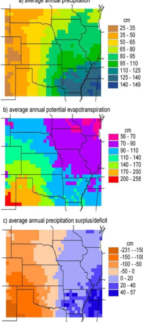
covers the entire United States at a resolution of one-half of one degree, meets many of the data needs of the model. Specifically, it contains monthly climate variables over the period 1895–1993, as well as information on soils and vegetation types. Figure 1a depicts the average annual precipitation in the VEMAP database for the period 1951– 1980 [as estimated by the Parameter-elevation Regressions on Independent Slopes

10

Model (PRISM; Daly et al., 1994)]. Figure 1b depicts the average annual potential evapotranspiration (PET) as calculated with the SW model using the LAI values deter-mined with the coupled models. We define PET as the sum of potential soil evapo-ration, potential transpiration and evaporation from canopy interception. As such it is not independent of either the type or the density (namely, LAI) of the vegetation. As

15

compared to a reference-crop calculation of PET (such as Penman’s (1948) original equation), the amounts in Fig. 1b cover a wider range, being greater (larger) in regions of small (large) LAI. The differences between annual average precipitation and PET (Fig. 1c) divide the study region longitudinally into dry and humid halves according to Thornthwaite’s (1948) classification of climate.

20

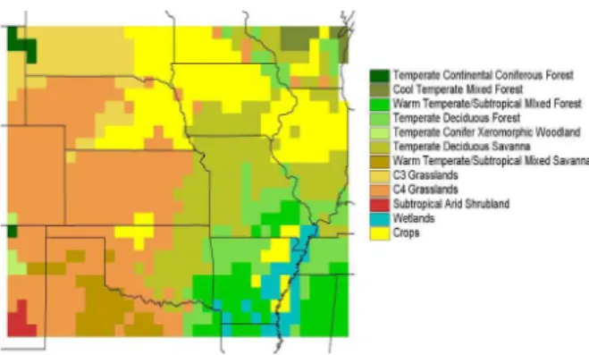
The VEMAP vegetation types are depicted in Fig. 2. A mask of grid cells that are pre-dominantly crops has been applied over the natural vegetation types. We also changed the natural vegetation class for a few cells to the dominant type of the surrounding cells in order to isolate individual vegetation classes to climatically similar regions. The dry half of the study region is dominated by grasses, savanna and shrubs, and the humid

25

half by forests, savanna and crops.

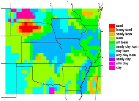
The USDA soil texture classes based on grid-cell averages of sand, silt and clay percentages in the VEMAP database are shown in Fig. 3. Considerable effort was

re-HESSD

Full Screen / Esc

Printer-friendly Version Interactive Discussion

quired to translate those percentages to values of the soil hydraulic parameters, as well as to develop a one-half-degree dataset of the parameters of the stochastic precipita-tion model from observaprecipita-tions of hourly precipitaprecipita-tion. Estimaprecipita-tion of parameter values and monthly climatic drivers are detailed below.

3.1 Soil hydraulic parameters

5

The soil hydraulic parameters in the SDEM are those of Brooks and Corey (1966), who formulate the dependency of the soil matric potential on soil moisture content as

Ψ(s) = Ψss−1/m (1)

where Ψ(s) is the soil matric potential at a relative soil saturation of s, Ψs is the

bub-bling matric potential (i.e., the value at which air entry begins), andm is the pore size

10

distribution index.s is defined by

s = θt− θr nt− θr

(2)

where θ_t is the total volumetric soil water content, θ_r is the residual volumetric soil water content, and n_t total porosity. Brooks and Corey formulate the dependency of the unsaturated hydraulic conductivity ons as

15

K (s) = Kssc (3)

wherec is the pore disconnectedness index, which the authors show to be related to the pore size distribution index by

c = 2 + 3m_m (4)

Grid-cell mean bulk density and percentages of sand, silt and clay from the VEMAP

20

database were used to estimate values of the Brooks-Corey soil hydraulic parame-ters. Those data are given for two soil layers: 0–50 cm and 50–150 cm, where the

HESSD

Full Screen / Esc

Printer-friendly Version Interactive Discussion

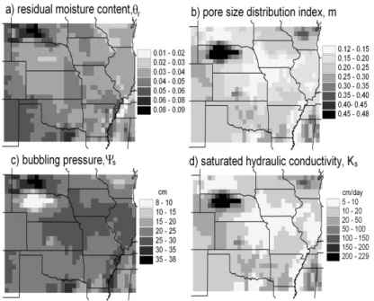
data for the former are used for root zone and the data for the latter are used for the recharge zone, regardless of the actual values used for the depth of the soil layers. Bulk density was converted to total porosity with the standard assumption of a mineral density of 2.65 g/cm3. Kochendorfer (2005) modeled the dependence of θ_r, Ψs and

m on soil texture by multivariate linear regression. The results of application of the

5

regression equations to the VEMAP sand and clay percentages for the 0–50 cm layer are presented in Fig. 4a–c. Following Rawls et al. (1982), Kochendorfer related the Brooks-Corey parameters toKs using an equation derived by Brutsaert (1967) based

on a permeability model developed by Childs and Collis-George (1950). The equation was scaled to fit the textural-class geometric means reported by Cosby et al. (1984)

10

and Rawls et al. (1982). Shown in Fig. 4d are the results for the root zone after a lower limit of 5.0 cm/d was placed onK_s.

3.2 Storm statistics

Kochendorfer (2005) derived monthly values for the statistics of the PRP precipitation model from hourly observations of precipitation as compiled by the National Climatic

15

Data Center (NCDC) and made available on CD-ROM by EarthInfo, Inc. (EarthInfo, 1999). Those observations were taken by recording rain gauges located at National Weather Service, Federal Aviation Administration, and Cooperative Observer stations. Thousands of these stations began making observations in and soon after 1948 and continue through the present. The 50-year period from 1949 to 1998 was selected for

20

estimation of the parameter values of the precipitation model. Stations in the NCDC database were included in the analysis if they have records for at least 40 of the 50 years and have no more than 20% missing data for the available years. Within an area extending 2.5◦ _{latitude and longitude beyond the boundaries of the study}

re-gion, 706 stations met those criteria. Ordinary kriging [detailed descriptions of which

25

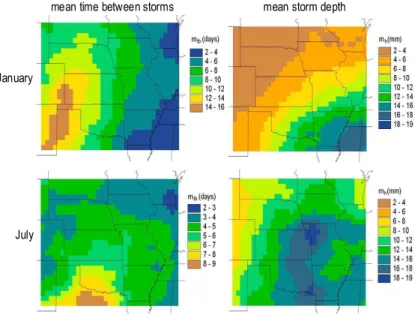
can be found elsewhere (e.g., Kitanidis, 1993)] was selected a priori as the preferred method for interpolating the station statistics to the half-degree grid of the study re-gion. The results for January and July are presented in Fig. 5 for two of the more

HESSD

Full Screen / Esc

Printer-friendly Version Interactive Discussion

important statistics: m_tb, the mean time between storms, andm_h, the mean depth of storms. The former primarily controls the frequency with which stage-two soil evapo-ration is reached, while the latter primarily controls the partitioning between infiltevapo-ration and surface runoff.

In an equilibrium calculation of the monthly water balance, the PRP statistics are

5

all that are needed (see Kochendorfer and Ramirez, 2008). In Eagleson’s application of his original model to estimating the interannual variability of runoff, he perturbs the model with variations in annual precipitation as sampled from its PDF (as predicted by the PRP model), while leaving the values of the PRP statistics alone (Eagleson, 1978g). However, a given value of precipitation over some period that is larger (smaller)

10

than long-term mean increases the likelihood of greater (fewer) number of storms for that time period, as well the likelihood for deeper (shallower) storms than the mean depth. By applying Bayes’ Theorem to the PRP model, Salvucci and Song (2000) derive probability distributions for the number of storms and the mean storm depth over a given period conditioned on the actual precipitation for that period. We use their

15

methodology to condition the monthly mean values of the PRP statistics in each month on the observed VEMAP/PRISM total for the given month and grid cell. Details can be found in Kochendorfer (2005).

3.3 Monthly climate variables

In addition to being the source of monthly precipitation, the VEMAP database provided

20

monthly mean temperatures, as well as two other variables necessary for implemen-tation of the SW model: incoming solar radiation and water vapor pressure. Four variables necessary for implementation of the SW model not included in the VEMAP database are net long-wave radiation, surface albedo, air pressure and monthly wind-speed (the last being provided only as a seasonal climatology). Net long-wave radiation

25

was estimated from cloudiness, surface temperature and humidity using a methodology outlined by Sellers (1965). Cloudiness was estimated as a linear function of the ratio of solar radiation incident at the surface to that incident at the top of the atmosphere, with

HESSD

Full Screen / Esc

Printer-friendly Version Interactive Discussion

the slope and intercept visually calibrated to maps of a climatology of observed percent sunshine (Baldwin, 1973). Surface albedo was taken from a gridded, monthly climatol-ogy created by Hobbins et al. (2001) based on Gutman (1988). Surface air pressure and surface windspeed were interpolated from monthly values produced by the NOAA-CIRES Center for the Diagnosis of Climate (http://www.cdc.noaa.gov/cdc/reanalysis/)

5

from results of the NCEP/NCAR reanalysis project (Kalnay et al., 1996). The remain-ing, water-vapor-related variables were calculated from vapor pressure, air temperature and air pressure using standard formulas presented by Shuttleworth (1993).

3.4 Green leaf area index

As discussed in Sect. 1, the peak in green LAI in the SW model is adjusted in each

10

year, within upper and lower bounds, such that the level of soil moisture at which the vegetation experiences water stress is just reached. LAI in each month is scaled by the same factor, thereby keeping the phenology (seasonal progression) of LAI fixed. To estimate that phenology, we use the multi-year LAI dataset of Buermann et al. (2002), which was derived from the Normalized Difference Vegetation Index (NDVI) as

mea-15

sured by Advanced High Resolution Radiometer (AVHRR). In addition to being publicly available at the half-degree resolution of the VEMAP data, we found it to be more rep-resentative of ground-based observations of peak green LAI over the study region than other datasets, most notably that of Los et al. (2000). From a version of the dataset posted by the authors athttp://cybele.bu.edu, we calculated monthly averages of green

20

LAI over the study region for the period July 1981 to June 1991 (Fig. 6). The upper bound in the dataset of six is the reason for using the same upper bound in the SW model.

Because the estimation of the interannual variability of LAI in the coupled model is predicated on water being the main limitation to growth, we examine the extent to which

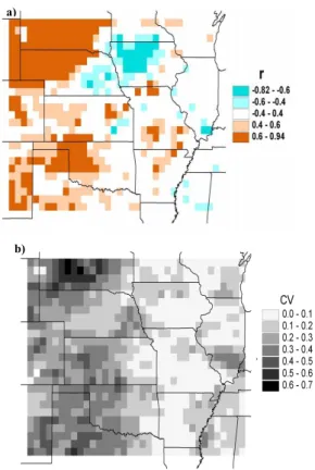
25

this is evident in observed LAI. Correlation coefficients between January-July total pre-cipitation and July observed LAI from 1980 to 1991 are depicted in Fig. 7a, along with the coefficients of variation in observed LAI in Fig. 7b. With a sample size of only ten,

HESSD

Full Screen / Esc

Printer-friendly Version Interactive Discussion

the confidence limits are wide, and so only values outside the range of –0.4 to 0.4 are shown. Over most of the grasslands region the correlation coefficients are greater than 0.5. Over most of the rest of the study area, values are scattered both positive and neg-ative. The exception is over the region of high crop density centered on west central Iowa (see Fig. 2), where the correlation is significantly negative. In their discussion of

5

the interannual variability of crop production in Iowa, Prince et al. (2001) note that two of the lowest levels of NPP occurred during a year with a very wet spring and one with summer flooding. Therefore, the negative correlation in that area may indeed be a real phenomenon. In general, the lack of significant positive correlation over cropped areas highlights the importance of management factors, such as fertilization and irrigation,

10

and climatic factors other than the availability of soil moisture. The low correlation and interannual variability in most of the humid half is likely in part due to the somewhat arbitrary upper bound of six in the observed LAI. To wit, ground-based observations of LAI as high as 10 have been made at the Coulee Experimental Forest in southwest Wisconsin (Scurlock et al., 2001). Nonetheless, the correlation results over the humid

15

half of the study region – along with the related fact that the coefficients of variation of observed LAI are generally low – suggest that it may be more appropriate to hold LAI at fixed values for crops and other vegetation for which water limitation is relatively unimportant on an interannual basis. However, the availability of water may still play a role in the long-term mean LAI of the vegetation in the humid half. The extent to which

20

this evident in model results is explored in Sect. 4.3.

It should be noted that since the Buermann et al. (2002) LAI data were acquired in the spring of 2002, the authors have posted a newer version on their website. Our comparison of that version with the original data showed it to contain significantly higher (by up to a factor of three for grasslands) averages of peak LAI over the study region.

25

It is suggested in Sect. 4.3 that the original data do in fact underestimate LAI over much of the grasslands, but not to the degree implied by the newer data. In addition, the authors believe that the newer data in general overestimate LAI (Myneni 2003, personal communication). In that light and in consideration of the evidence for the

HESSD

Full Screen / Esc

Printer-friendly Version Interactive Discussion

representativeness of the original data presented in Buermann et al. (2002), we elected to continue to use their original data. Again we note that the LAI observations are used only to provide a fixed phenology of green LAI, which is scaled by a single factor. 3.5 Parameter values specific to vegetation class

Parameters values specific to each of the 12 VEMAP vegetation classes in the study

5

region are listed in Table 1. Sources for parameter values are identified in the table and include other modeling studies, field studies and literature surveys. The precision applied to estimating a parameter value was a function of the availability, range and uncertainty of values in the literature, as well as of the sensitivity of model results to the given parameter. Many values, such as canopy height and leaf width, are only order

10

of magnitude estimates. Careful consideration was given to the monthly timescale at which the model is implemented, especially with regard torsmin, the minimal stomatal

resistance. In selecting parameter values, we also considered the degree to which vegetation classes other than the designated one are present. For example, much of the area parameterized as wetland and temperate deciduous savanna is cultivated

15

cropland. Significant calibration was performed for the values of only two parameters: rsminandrss, the soil-surface resistance. In initially estimating values ofrss, we took the

view that they are mainly due to the litter layer. The calibration process consisted mainly of visually matching modeled mean annual runoff to contours of observed streamflow. All parameters values were kept well within their range of uncertainty, and their original

20

rank by vegetation class was preserved.

As the main determinant of the absolute amount of water available for transpiration, the root zone depth,z_u, is one of the more important parameters in SVAT models (Jack-son et al., 2000; Mahfouf et al., 1996). The distribution of roots below a given stand of vegetation is a complex function of plant speciation and phenology, chemical and

25

physical properties of the soil, and climate. Many of those factors converge to produce similar root distributions within a given biome (Schenk and Jackson, 2002). Jackson et al. (1996) compiled a database of 250 root studies, which they grouped into 11 biomes.

HESSD

Full Screen / Esc

Printer-friendly Version Interactive Discussion

They fit an exponential equation to plots of cumulative root fraction versus soil depth within each biome. We used the resulting decay constants to calculate root zone depth as the depth that contains 95% of the root biomass. Because temperate savanna and wetlands are not amongst the biome classes used by Jackson et al. (1996), we se-lected values intermediate between grasses and forests. Likewise, the root zone depth

5

of conifer woodland was taken as intermediary between that of savanna and forest. Evapotranspiration estimates with the model are much less sensitive to the depth of the recharge zone, zd, which mainly controls the phase and amplitude of the annual

cycle in groundwater recharge. A recharge zone of about twice the depth of the root zone gave seasonality in groundwater recharge (and hence base flow) consistent with

10

the observed seasonality in streamflow across the study region (e.g., Geraghty and Miller, 1973). Accordingly, values for z_d of 100, 150 and 200 cm were assigned to vegetation classes based on the closest match to twice the corresponding value ofz_u. As the determinant of the moisture content at which transpiration begins to decrease below the potential rate (and consequently a determinant of the peak in green LAI), the

15

critical soil matric potential, Ψuc, is also a relatively important parameter. That such a

point exists is based on a resistance model of transpiration typically attributed to Cowan (1965), following the work of Gardner (1960) and van den Honert (1948). The model indicates that Ψucshould be a function of the transpirative demand of the atmosphere,

as well as the density of the roots and of the transpiring leaf area. Rather than try

20

to estimate the resistances in the Cowan model, we assume that Ψuc is relatively

invariant within given climatic regions and associated vegetation classes at the time of the year when water stress is most likely to occur. Assuming fixed values of Ψuc is

fairly common in the modeling of transpiration (Guswa et al., 2002).

4 Results and discussion

25

As noted above, we calibrated the soil surface resistances and minimum stomatal re-sistances of the SW model by vegetation class via a visual fit of modeled mean annual

HESSD

Full Screen / Esc

Printer-friendly Version Interactive Discussion

runoff to contours of observed streamflow. Because the streamflow contours were de-veloped as an average for the period 1951–1980 (Gebert et al., 1987), we used that 30-yr period. No separate validation period is examined. Rather, the validity of the model is established through the realism with which it reproduces not only runoff but also all other components of the water balance, including soil moisture, green LAI, soil

5

evaporation and transpiration. 4.1 Annual runoff

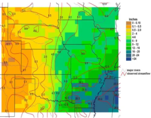
The contours of observed streamflow overlay modeled annual runoff in Fig. 8. An ex-cellent match to overall climatic trends was obtained. The model even does a reason-able job of capturing the higher runoff over the topographically complex Black Hills and

10

Ozark Mountains based on grid-cell average climate alone. Nonetheless, for a num-ber of individual cells and small clusters of cells with runoff greater than two inches, differences between the contours and model results are as high as about ±50%. In addition, on a relative basis, the model substantially overestimates streamflow over most of the driest part of the study region (i.e., New Mexico and the Texas and

Okla-15

homa panhandles.) This is likely due to an overestimate in surface runoff in the region (Kochendorfer, 2005). Many other reasons could be cited for the differences between observed stream flow and modeled runoff. Some of the most significant not associated with measurement and interpolation error in the contours, nor with error in the water balance model, have to do with scale and the fact that runoff calculated from

stream-20

flow may not necessarily be representative of actual watershed runoff. In general, the one-dimensional form of the SDEM and its lack of interaction with groundwater is a significant limitation to predicting runoff and streamflow at basin scales. However, our main interest in comparing modeled runoff and observed streamflow is as a validation of modeled evapotranspiration for a typical upland site within each grid cell. In that

25

HESSD

Full Screen / Esc

Printer-friendly Version Interactive Discussion

4.2 Soil moisture

We identified four sets of long-term records of observed soil moisture encompassing a range of climatic conditions across the study region. The first two datasets come from two grassland sites in the Great Plains: the Central Plains Experimental Range (CPER) in north-central Colorado and the USDA-ARS R-5 experimental watershed

5

near Chickasha, Oklahoma. Those two sites are used by Kochendorfer and Ramirez (2008) to test the LAI-optimization hypothesis with the coupled models. The third set of soil moisture data comes from another USDA-ARS experimental watershed: an 83-acre cropped watershed near Treynor, Iowa, designated as W-2. The collection of soil moisture data from W-2 lasted from 1972 until 1994. Those data, as well as the fourth

10

dataset, were downloaded from the Global Soil Moisture Data Bank (Robock et al., 2000). The fourth and final set of soil moisture data is from the Illinois Climate Network (Hollinger and Isard, 1994). We used the data from 1983 to 2001 for 15 soil-moisture stations that are grass covered and located in the silt loam and silty clay loam soils that dominate the state.

15

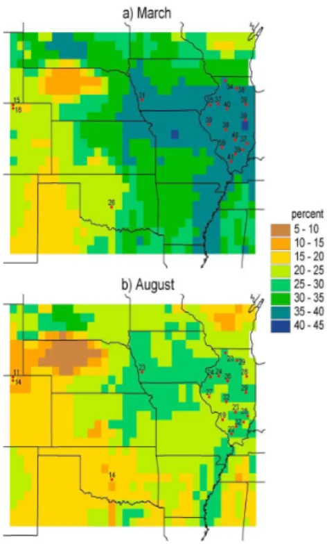
The observations of mean root-zone (as defined by the values ofzuin Table 1)

volu-metric soil moisture over the given periods of record are plotted on top of model results in Fig. 9 for March (with the exception of the Iowa site, for which April is plotted due to the lack of March measurements) and August. Those months are the respective months in which modeled soil moisture most frequently reaches its annual maximum

20

and minimum. Based on the plots, large-scale variations in the magnitude and sea-sonality of moisture content appear to be captured by the model. The influence of soil texture is seen throughout the study region, mostly noticeably in the differences in moisture content between the Sand Hills of north-central Nebraska and the Pierre Shale Plains of south-central South Dakota. In the CPER observations, the

signifi-25

cance of subgrid variability in soil texture is seen in the higher moisture retention of the clay-loam soil in comparison to the sandy-loam soil (where the latter has been plotted above the former). Over Illinois, there is no clear spatial structure to either observed or

HESSD

Full Screen / Esc

Printer-friendly Version Interactive Discussion

modeled soil moisture. Apparently, the slight north-to-south increase in annual precip-itation over Illinois is more-or-less completely offset by the north-to-south increase in potential evapotranspiration. For both March and August, using the t-test for unequal variances, there is no significant difference at the 95% confidence level between the mean of the 15 observed values and the mean of modeled values for the grid cells in

5

which the observations fall. Finally, we note that in contrast to that for the two grass-land sites, modeled mean August soil moisture values for the Iowa and Illinois sites are somewhat above the critical value, indicating that in many years the model reaches the maximum peak green LAI of six.

4.3 Model-determined leaf area index and above-ground net primary productivity

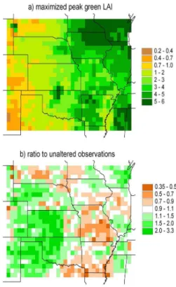
10

Figure 10 depicts the 30-yr averages of model-determined peak green LAI and com-pares them to the unaltered NDVI-based observations. The model-determined LAI preserve the general climatic trend of increasing LAI with increasing humidity, while largely missing more regional-scale variations. The model-determined LAI tend to be higher than the unaltered observations in the drier regions and lower in the wetter

15

regions. As a whole, the model-determined LAI, with a mean of 2.79 and standard de-viation of 1.61, tends to be slightly larger and slightly less variable than the unaltered observations, which possess a mean of 2.66 and a standard deviation of 1.78. Given the uncertainties in the NDVI-based observations discussed in Sect. 3.4, we cannot assume that the unaltered observations are a more accurate representation of actual

20

LAI. Using ground-based observations and productivity data, we examine below the likely accuracy of the model-determined LAI as compared to the unaltered observa-tions. Our primary interest is with the water-limited grasslands of the western half of the study region.

Because of the labor-intensive nature of data collection, ground-based observations

25

of LAI are sparse. Scurlock et al. (2001) compiled a global dataset of field-measured LAI as reported by numerous researchers. Several sites contained in that dataset are located within the study region of this paper. For the most part, those sites are

HESSD

Full Screen / Esc

Printer-friendly Version Interactive Discussion

in grid cells where there is generally good agreement between the model-determined peak in green LAI and the unaltered NDVI-based observations. Taken together with their limited spatial and temporal extent, the values reported at nearly all the sites are uncertain and varied enough that both the model-determined LAI and the unaltered observations can be assessed comparable to the field measurements.

5

Over the humid half of the study area, the differences between the model-determined peak in green LAI and the unaltered observations show some spatial structure (Fig. 10b). The greatest association with vegetation type or soil texture is a low bias in the model-determined values in lower Mississippi River valley, which is dominated by crops and wetlands over silty clay loam soils (see Figs. 2 and 3). We were unable

10

to find ground based observations of LAI in this region. Both raw NDVI data and the unaltered NDVI-derived LAI observations in Fig. 6, show it to be a region of lower pro-ductivity. However, actual mean peak LAI may not be as low as the 1–2 range predicted by the model, indicating that the soil hydraulic parameters or the critical matric potential for crops and wetlands, or both, may produce a higher than actual value of the

criti-15

cal soil moisture content. Furthermore, the fact that the difference between modeled and observed peak LAI in the humid half of the study region is relatively unbiased in the mean is likely due to the upper bound being 6. Therefore, vis- `a-vis the discussion above and in Sect. 3.4, we cannot conclude that the use of the critical matric potential to estimate peak green LAI during years in which water may be limiting improves the

20

unaltered NDVI-based observations in the humid half of the study region

As seen in Fig. 10b, the model-determined LAI are greater than the unaltered ob-servations over most of the grassland region. The area of greatest disagreement is centered midway along the border between Nebraska and Oklahoma. The dataset of Scurlock et al. contains LAI measurements at two sites within this area. The first is

25

an LAI of 7.5 for a 1997–1998 harvest of a wheat crop located at 36.75◦N 97.08◦W. For the corresponding grid cell, which is parameterized as C₄ grasses, the model-determined LAI is 5.9, indicating that for most years the upper bound of 6.0 is reached. In contrast, the unaltered NDVI-derived peak in green LAI is only 2.1. The second

HESSD

Full Screen / Esc

Printer-friendly Version Interactive Discussion

site is located in the adjacent grid cell to the east at 36.85◦_{N 96.68}◦_{W. The vegetation}

there is reported as grass, with two undated LAI measurements of 5.4 and 5.8. For the grid cell, the model-determined LAI is 2.1, and the unaltered NDVI-derived peak is 1.9. We suspect that the field measurements are biased towards the high side, but nonetheless, they suggest a region of higher productivity. Also indicative of the

poten-5

tial for higher productivity is the fact that a group of seven cells just to the west of the field measurements are mostly in crops (see Fig. 2). Located at the southern end of the area of higher model-determined LAI, at 35.15◦N 97.75◦W, is the R-5 experimental watershed. For this grassland catchment, two hydrologic modeling studies were found that use field-based estimates of peak green LAI of 2.5 (Ritchie et al., 1976) and 3.2

10

(Luxmoore and Sharma, 1980). For the corresponding grid cell, the model-determined LAI is 2.1, and the unaltered NDVI-derived observation is 1.1 – further evidence that the latter underestimates peak green LAI in this area of the grasslands.

Given the paucity of field-measured LAI, we turn to another measure of vegetation density, aboveground net primary production (ANPP). Zheng et al. (2003) integrated

15

15 studies containing mostly empirical estimates of net primary productivity (NPP) for a variety of terrestrial biomes across the globe. The end product of that effort is a one-half-degree gridded dataset of ANPP and total NPP (TNPP). Of relevance to the present study, estimates of grassland productivity are provided over most of the US Great Plains. The sources of those data are three studies using grassland

productiv-20

ity data from the USDA Natural Resource Conservation Service. The most spatially extensive is that of Tieszen et al. (1997), who correlated potential rangeland produc-tion estimates with NDVI data from 1989 to 1993 to estimate ANPP at a one-kilometer resolution for 13 major grassland seasonal land cover classes. In Fig. 11a, the model-determined peak in green LAI values for those cells designated as grassland in the

25

model parameterization are plotted against the corresponding Tieszen et al. (1997) estimates of ANPP (as resampled to the half-degree grid by Zheng et al., 2003). The unaltered observations of peak-green LAI are plotted against the ANPP estimates in Fig. 11b. Based on a power curve fit, the ANPP data is substantially more correlated

HESSD

Full Screen / Esc

Printer-friendly Version Interactive Discussion

to the model-determined LAI (R2=0.59) than to the unaltered observations (R2=0.42). We note that both the LAI observations and the ANPP estimates are derived from the NDVI data – albeit in very different ways. For this reason, the higher correlation be-tween LAI and ANPP brought about by the model adjustment is a particularly strong endorsement of that process for water-limited grasslands.

5

The most distinct exceptions to the trend in the grasslands region of a model-determined LAI larger than the unaltered observations are the high-clay-content re-gions of the Pierre Shale Plains and east-central Texas (see Fig. 3). In contrast to the Pierre Shale Plains, where the grid cells contain the highest percentages of clay within the larger study region, the Sand Hills region is the locus of the highest

per-10

centages of sand. Over the entire Sand Hills region the model-determined LAI are larger than the observations, with the ratio greater than two for a few of the cells. The contrast in model-determined LAI between the two regions is reflected in the Tieszen-et-al. ANPP data; in the Pierre Shale Plains, ANPP generally falls in the range of 60 to 110 g/cm2, while in the Sand Hills, it generally falls in the range of 120 to 170 g/cm2

15

(see Fig. 13b for a plot of the TNPP data, which are derived from the ANPP data.) The model-determined LAI in the corresponding grid cells range from 0.7 to 0.9 and 1.3 to 1.9, respectively – the same approximate one-to-two ratio as ANPP. In contrast, the unaltered observations of peak green LAI (see Fig. 10) are actually higher over the Pierre Shale Plains than over the Sand Hills. That the model reproduces the higher

20

productivity of the Sand Hills suggests that it is able to capture the inverse texture effect (Noy-Meir, 1973). Kochendorfer and Ramirez (2008) evaluate that ability more rigorously using model results for the CPER site and the R-5 watershed

We cannot compare the model-determined LAI against the unaltered observations without addressing the impact of land use. Grazing is the predominant land use in the

25

grasslands region. The significance of grazing intensity can be seen in comparison of the R-5 catchment, which was moderately grazed, with the adjacent R-7 catch-ment, which has similar soils but was intensely grazed. As a result of the overgrazing and subsequent erosion, the vegetation cover was significantly smaller over the R-7

HESSD

Full Screen / Esc

Printer-friendly Version Interactive Discussion

catchment; Ritchie et al. (1976) indicate a peak green LAI value of 0.5 for the R-7 catchment, and Luxmoore and Sharma (1980) report a value of 0.75. The model-determined LAI may thus be more representative of a “potential” LAI, which would be achieved in the absence of overgrazing, fire, infestation, disease or other significant disturbances (e.g., Nemani and Running, 1995). At least some of the difference

be-5

tween the model-determined LAI and the unaltered observations over the grasslands is then attributable to one or more of those disturbances, grazing being the most likely culprit on a long-term basis.

Second in importance in the grasslands to grazing is crop production. While only a handful of cells within the grassland region are designated as crops in the model

10

parameterization, crops are raised throughout. For example, the April and May peak in green LAI over much of the central and southern grasslands (see Fig. 2) is an in-dication of the prevalence of winter wheat there. Because it occurs when transpira-tional demand is still relatively low, the early peak in fact allows for the relatively high model-determined LAI in this region. The model-determined LAI may thus be more

15

representative of wheat than the more predominant grasslands. On the other hand, management factors, such as fertilizer application and irrigation, likely play a role in the model-determined LAI underestimating the observed grid-cell averages. In fact, many of the cells in the grassland region where the model-determined LAI is less than the unaltered observations correspond to areas of high levels of irrigation (USGS, 1993).

20

These areas include the plains along the Front Range of the Rocky Mountains and around the Black Hills, and the Platte River valley in southern Nebraska. Other areas of intense irrigation appear as just localized reductions in the generally high ratio be-tween the model-determined LAI and the unaltered observations. These areas include a few cells in the southwest corners of Kansas and the Texas panhandle (see Fig. 10b).

25

4.4 Potential and actual soil evaporation

Results from application of the SW model to the calculation of potential rates of soil evaporation with model-determined LAI are depicted in Fig. 12a–c for March, August

HESSD

Full Screen / Esc

Printer-friendly Version Interactive Discussion

and for the sum of all months. The results for March, when green LAI is low or nonex-istent, are primarily controlled by the latitudinal temperature gradient. The results for August, being higher in areas of lower LAI, are indicative of the growing season (see Fig. 10a). Because evapotranspiration takes place predominantly in the growing sea-son, a similar pattern is seen for the annual totals. Actual soil evaporation is depicted

5

in Fig. 12d–f as depths, and in Fig. 12g–i as a percentage of the potential. In the humid half of the study region in March, soil evaporation is virtually always under climate con-trol (i.e., stage-two evaporation is seldom reached) as a result of the seasonally high moisture content and low potential soil evaporation. As one moves to the southwestern corner, the degree of soil control rapidly increases to the point of being almost entirely

10

limited by the availability of soil moisture (i.e., stage-two evaporation is reached soon after the end of storms.) In August, when potential rates are at or near their highest and soil moisture values at their lowest, most of the dry half of the study region undergoes strongly soil-moisture-limited evaporation.

Figure 13 depicts total evapotranspiration and the percentage that is soil

evapora-15

tion for July and for the entire year. The remaining percentages are dominated by transpiration, with canopy interception accounting for no more than about 10% on both a seasonal and annual basis. In July, when green LAI is at or near its peak, soil evap-oration falls in the range of 10% to 30% of total evapotranspiration for the majority of the cells, with the percentages being more variable in the dry half of the study region.

20

On an annual basis, soil evaporation comprises between 30% and 60% of total evapo-transpiration for nearly all the cells. The distribution of percentages shows surprisingly little correlation to vegetation class or climate. This suggests that the generally lower vegetation cover and lower soil-surface resistances in the dry half of the study region are more-or-less completely offset by the drier soil.

25

In contrast to vegetation class and climate, the influences of soil texture are clear in the percentages in Fig. 13. The differences in LAI resulting from the differences in soil texture between the Pierre Shale Plains and the Sand Hills manifest themselves as, respectively, regionally higher and lower percentages of soil evaporation. In the

HESSD

Full Screen / Esc

Printer-friendly Version Interactive Discussion

humid half of the study region, the highest percentages of soil evaporation (i.e., those in excess of 60%) are associated with the high-clay soils of the lower Mississippi River valley and Northeast Texas (see Fig. 3). The proximate cause of these higher percent-ages is also the greater potential soil evaporation (see Fig. 12b, c) that results from the regionally lower LAI (see Fig. 10a). This might suggest that the inverse texture effect

5

is also in operation here, in the humid half of the study region. However, based on soil texture, the available water capacity of the corresponding cells is actually lower than in the surrounding cells. Furthermore, if we look at soil evaporation as a percentage of potential soil evaporation (see Fig. 12g–i), we see that the percentages are slightly higher than the surrounding cells in the high clay areas of the humid half, while slightly

10

lower in the Pierre Shale Plains. This suggests that the lower diffusivity of the high-clay soils has a greater offsetting effect to the higher moisture content in the Pierre Shale Plains than in the humid regions. The difference has mainly to do with the degree to which soil evaporation is controlled by moisture content; in the humid half of the study region, at least 60% of the potential demand is met for nearly all the cells on an annual

15

basis.

Although relatively new isotopic, sap-flow and eddy-covariance methods are increas-ingly being applied (e.g., Smith and Allen, 1996), separate observation of soil evapora-tion and transpiraevapora-tion has historically been difficult, and continues to be, particularly at the stand and larger scales, and over time periods representative of average climatic

20

conditions. Therefore, there are not many data that can be used to validate the par-titioning of evapotranspiration in the model results. Nonetheless, a few studies were identified at sites in or near the study region. Of particular interest are the stable iso-tope study of Ferretti et al. (2003) and the energy-balance measurement and modeling study of Massman (1992) conducted at the CPER. Those studies were reviewed by

25

Kochendorfer and Ramirez (2008) and found to be in good agreement with model re-sults for the CPER. Their SDEM-SW rere-sults show that, over the growing season, soil evaporation is the dominant component of evapotransiration in April and May and a neglible component in August and September, with the June and July percentages

ap-HESSD

Full Screen / Esc

Printer-friendly Version Interactive Discussion

proximating the average over the whole growing season. Even in the sparse canopy of the shortgrass steppe, measured peak LAI at the CPER ranges from 0.4–0.6 (Hazlett, 1992; Knight, 1973), growing-season soil evaporation appears to average one third or less of total evapotranspiration. Measurement-based studies from more arid environ-ments in the southwest USA (Dugas et al., 1996; Stannard and Weltz, 2006) indicate

5

that transpiration dominates there as well.

In comparison, to natural vegetation, more evapotranspiration partitioning studies have been conducted of crops, with a tendency to focus on irrigated systems. The cu-mulative impression from several such studies (Ashktorab et al., 1994; Klocke, 2003; Leuning et al., 1994; Massman and Ham, 1994; Peters and Russell, 1959; Villabalobos

10

and Fereres, 1990), as well as from a review paper (Burt et al., 2005), is that cumulative growing-season soil evaporation ranges from 20% to 50% of total evapotranspiration for well-watered crops–both irrigated and rain-fed. Thus crop percentages in the litera-ture are similar to those for semi-arid grasslands and also in good agreement with the model results in Fig. 13 (which were produced under the assumption of rain-fed crops.)

15

Variations in the literature values appear to be more dependent on irrigation and tilling schemes than on climate or crop type.

Finally, we consider the empirical data on evapotranspiration partitioning in forests in the humid half of the study region. Eddy covariance measurements in deciduous forests near the eastern edge of our study region (Grimmond et al., 2000; Wilson et al.,

20

2001) show evaporation from the forest floor to be about 10% of total evapotranspiration at peak LAI. Because model results in Fig. 13 show a contribution in July from soil evaporation of 10–30%, we can conclude that the model tends to overestimate soil evaporation in humid forests. This may be the result of the upper bound on LAI being limited to six. Another possible source of model error is the values of surface soil

25

resistance for forests in Table 1 underestimating the mulching effect of the litter layer. In general, greater consideration needs to be given to the limitations of applying the two-component SW model (which was originally developed for sparse crop canopies) to the taller and generally heterogeneous, multi-leveled canopies of forests, woodlands

HESSD

Full Screen / Esc

Printer-friendly Version Interactive Discussion

and savannas.

4.5 Transpiration, total net primary productivity and water use efficiency for the grass-lands

We further validate the partitioning of evapotranspiration in the grasslands through the calculation of water-use efficiency (WUE), which (by the definition that we use among

5

many possible) measures total plant production per amount of water transpired. The grassland productivity data in the NPP database of Zheng et al. (2003) are particularly useful in this regard. Of most interest, Tieszen et al. (1997) combined their ANPP data with below-ground NPP calculated using an algorithm derived by Gill et al. (2002).

We re-ran the model for the base 30-yr period with all the cells for which the native

10

vegetation is C3 or C4 grassland parameterized as such. Cells in which the native

vegetation is either one of the two savanna classes were also parameterized as C₄ grassland. By dividing the TNPP values (Fig. 14b) by the corresponding values of annual transpiration (Fig. 14a) in cm and multiplying by 0.1, we arrived at WUE in units of g-C/kg-H₂O (Fig. 14c). For the C₄grasslands, the pattern is one of increasing WUE

15

as one moves out from the southwest (i.e., in the direction of increasing humidity.) This is consistent with the physiology behind WUE; using a resistance model of the diffusion of CO₂ and water vapor across stomata, Kramer (1983) shows that WUE is inversely proportional to the difference in the vapor pressure of water inside and outside the leaf. The four cells of very high water-use efficiency in Northeast Texas are probably

20

mostly the result of the soil hydraulic parameters underestimating the plant-available water of the associated silty clay soils. That LAI (and hence transpiration) has been underestimated in this region is also suggested by Fig. 10b.

Despite the clear climatic dependence of WUE, generalized values for specific species or classes of vegetation can be found scattered throughout the plant

physi-25

ology literature. Based on a number of sources, Larcher (1980) presents single values and ranges of values for “transpiration ratios” categorized by life form, photosynthetic pathway and species. For C₃grains and C₄plants, the author lists ranges of 500–650

HESSD

Full Screen / Esc

Printer-friendly Version Interactive Discussion

and 220–350 “liters of transpired water per kg of dry matter produced,” respectively. Us-ing a conversion factor of 0.45 g-C per g-dry matter (Zheng et al., 2003), those ranges correspond to WUE of 0.69–0.90 and 1.3–2.0 g-C/kg-H2O, respectively. Although the

focus of the WUE values presented by Larcher is more on cultivated crops than on pasture grasses, we might assume that the WUE of C₃ grasses fall somewhere in the

5

former range and those of C4grasses fall in the latter range. The relative productivity

of C3 and C4 grasses across the western half of the Great Plains varies along a

pri-marily north-to-south gradient, such that, for those cells in the study region designated as C4grassland, the relative productivity of C4species ranges from near 100% in

cen-tral Texas to around 50% in the northern Nebraska, while for the C3-grassland cells, it

10

varies from 50% in northern Nebraska to 20% in central South Dakota (Epstein et al., 1997a). If we approximate the average relative productivity of C4 grasses to be 35%

in the C3 cells of the study region and 75% in the C4 cells, then we expect WUE to

fall in the range of 0.90 to 1.29 g-C/kg-H₂O for the C₃grasslands and in the range of 1.15 to 1.73 g-C/kg-H2O for the C4 grasslands. The mean and standard deviation of

15

the calculated WUE are 1.06 and 0.25, respectively, for the C3 grasslands and 0.86

and .31, respectively, for the C₄grasslands. The WUE for the C₄grasslands are lower than for the C3 grasslands despite their higher stomatal resistance in the model

pa-rameterization (see Table 1). We might take those results as an indication that the model overestimates transpiration for C₄ grasslands (possibly due to overestimating

20

LAI, vis- `a-vis Fig. 10b). Alternatively, the TNPP estimates of Tiezsen et al. (1997) may be biased low; the database of Zheng et al. (2003) also contains grassland TNPP es-timates from the study of Sala et al. (1988) for about fifty scattered grid cells, which on average run 75% of the corresponding estimates from Tiezsen et al. (1997). Equally plausible, however, is that the ranges of WUE reported by Larcher are more

represen-25

tative of humid climates, especially because they are crop-based values. In fact, the calculated WUE for C4 grid cells that are on the more humid side of the grasslands

HESSD

Full Screen / Esc

Printer-friendly Version Interactive Discussion

5 Summary and conclusions

The SDEM as coupled to the SW canopy model has been applied to the central United States over a half-degree grid using vegetation, soil and climate data from the Veg-etation/Ecosystem Modeling and Analysis Project (VEMAP), among other sources. An excellent match of modeled mean annual runoff to contours of streamflow was

5

achieved with only minimal calibration of two evapotranspiration parameters, indicating that mean annual evapotranspiration is approximated well by the coupled models.

The interannual variation in LAI is modeled through application of the hypothesis that, in any year in which water is significantly limiting, vegetation will draw soil mois-ture down in the latter half of the growing season approximately to the point at which

10

the vegetation just begins to experience water stress. The hypothesis is applied to maximize the annual peak in green LAI, within upper and lower bounds, by scaling the seasonal LAI curve by a single factor. Grid-cell specific curves were determined from NDVI-based estimates of green LAI. For the water-limited grassland region, com-parison of the means of model-determined peak green LAI and those of the unaltered

15

NDVI-based observations with ground-based observations of LAI and with a gridded datasets of above-ground net primary production indicated that the model-determined values are at least as accurate as the unaltered observations. The lack of positive correlation between accumulated precipitation and the peak in observed green LAI for vegetation in the humid half of the study region suggest that the optimization

hypothe-20

sis is of limited use in this region. However, the somewhat arbitrary upper bound of six in both observed and modeled green LAI may be masking greater spatial and interan-nual variability and, consequently, the role of water in determining the long-term mean peak, particularly in the forested areas.

The partitioning of evapotranspiration in model results showed little dependence on

25

climate and vegetation type, with most of the variation across the study region at-tributable to soil texture and the resultant differences in vegetation density. The im-plication is that the higher (lower) soil moisture content in wetter (drier) climates is