Magnetically dominated structures as an important component of the solar wind turbulence

HAL Id: hal-00318855

https://hal.archives-ouvertes.fr/hal-00318855

Submitted on 29 Aug 2007

HAL is a multi-disciplinary open access

archive for the deposit and dissemination of

sci-entific research documents, whether they are

pub-lished or not. The documents may come from

teaching and research institutions in France or

abroad, or from public or private research centers.

L’archive ouverte pluridisciplinaire HAL, est

destinée au dépôt et à la diffusion de documents

scientifiques de niveau recherche, publiés ou non,

émanant des établissements d’enseignement et de

recherche français ou étrangers, des laboratoires

publics ou privés.

Magnetically dominated structures as an important

component of the solar wind turbulence

R. Bruno, R. d’Amicis, B. Bavassano, V. Carbone, L. Sorriso-Valvo

To cite this version:

R. Bruno, R. d’Amicis, B. Bavassano, V. Carbone, L. Sorriso-Valvo. Magnetically dominated

struc-tures as an important component of the solar wind turbulence. Annales Geophysicae, European

Geosciences Union, 2007, 25 (8), pp.1913-1927. �hal-00318855�

www.ann-geophys.net/25/1913/2007/ © European Geosciences Union 2007

Annales

Geophysicae

Magnetically dominated structures as an important component of

the solar wind turbulence

R. Bruno1, R. D’Amicis1, B. Bavassano1, V. Carbone2, and L. Sorriso-Valvo3

1_{INAF-Istituto Fisica Spazio Interplanetario, 00133 Roma, Italy}

2_{Dipartimento di Fisica Universit`a della Calabria, 87036 Rende (Cs), Italy} 3_{LICRYL – INFM/CNR, 87036 Rende (Cs), Italy}

Received: 21 February 2006 – Revised: 16 July 2007 – Accepted: 23 July 2007 – Published: 29 August 2007

Abstract. This study focuses on the role that magnetically

dominated fluctuations have within the solar wind MHD tur-bulence. It is well known that, as the wind expands, magnetic energy starts to dominate over kinetic energy but we lack of a statistical study apt to estimate the relevance of these fluc-tuations depending on wind speed, radial distance from the sun and heliographic latitude. Our results suggest that this kind of fluctuations can be interpreted as non-propagating structures, advected by the wind during its expansion. In particular, observations performed in the ecliptic revealed a clear radial dependence of these magnetic structures within fast wind, but not within slow wind. At short heliocentric distances (∼0.3 AU) the turbulent population is largely dom-inated by Alfv´enic fluctuations characterized by high values of normalized cross-helicity and a remarkable level of energy equipartition. However, as the wind expands, a new-born population, characterized by lower values of Alfv´enicity and a clear imbalance in favor of magnetic energy becomes visi-ble and clearly distinguishavisi-ble from the Alfv´enic population largely characterized by an outward sense of propagation. We estimate that more than 20% of all the analyzed intervals of hourly scale within fast wind are characterized by normal-ized cross-helicity close to zero and magnetic energy largely dominating over kinetic energy. Most of these advected mag-netic structures result to be non-compressive and might rep-resent the crossing of the border between adjacent flux tubes forming, as suggested in literature, the advected background structure of the interplanetary magnetic field. On the other hand, their features are also well fitted by the Magnetic Field Directional Turnings paradigm as proposed in literature.

Keywords. Interplanetary physics (Plasma waves and

tur-bulence; Solar wind plasma) – Space plasma physics (Turbu-lence)

Correspondence to: R. Bruno (bruno@ifsi-roma.inaf.it)

1 Introduction

Belcher and Davis Jr. (1971) introduced, for the first time, the concept that propagating Alfv´en modes could be inter-mixed with static structures advected by the solar wind. This idea came out from the observational evidence that Alfv´enic correlations were less pure within slow velocity regions com-pared to high velocity streams. Afterwards, several authors corroborated this concept using additional experimental ev-idences (Bruno and Bavassano, 1991; Klein et al., 1993; Bruno and Bavassano, 1993) which showed that a high de-gree of Alfv´enicity, intended as correlation between field δb and velocity δv fluctuations, is generally correlated with low compressibility of the medium although, in some cases, compressibility is not the only cause for a low Alfv´enicity (Roberts et al., 1991, 1992; Roberts, 1992).

Detailed studies performed by Matthaeus et al. (1990) on the two-dimensional correlation function of solar wind fluc-tuations at 1 AU, generally known in literature as the “Mal-tese Cross”, showed that interplanetary turbulence was made of two primary ingredients, namely Alfv´enic fluctuations and 2-D turbulence. This two-dimensional turbulence is charac-terized for having both the wave vector k and the perturb-ing field δb⊥ to the ambient field B0. However, given that the analysis did not separate fast from slow wind, it is likely that most of the the slab (Alfv´enic) correlations came from the fast wind while the 2-D correlations came from the slow wind. Anisotropic turbulence has been studied both theo-retically (Montgomery, 1982; Zank and Matthaeus, 1992) and through numerical simulations (Shebalin et al., 1983; Oughton et al., 1994). In particular, these simulations fo-cused on non-linear spectral transfer within MHD turbulence in presence of a strong mean magnetic field. It was ob-served that a remarkable anisotropy is created during the tur-bulent process and much of the power is transferred to fluc-tuations with higher k_⊥and less to fluctuations with higher k_k. Further theoretical models (Marsch and Tu, 1989; Tu and

Marsch, 1990; Zhou and Matthaeus, 1989) showed that the existence of 2-D non compressive turbulence comes out nat-urally from the structure of the transport equations. Bieber et al. (1996) formulated an observational test to distinguish the slab (Alfv´enic) from the 2-D component within interplan-etary turbulence. Several tests conducted by these authors as-signed a fraction of ∼80% to the 2-D component and the re-maining percentage to the Alfv´enic or slab component. How-ever, data used for this analysis were recorded near times of solar energetic particle events. Moreover, most of the data belonged to slow solar wind (Wanner and Wibberenz, 1993) and as such, this analysis is not representative of the whole phenomenon of turbulence in the solar wind. As a matter of fact, using Ulysses observations at high latitude, when the s/c was imbedded in the polar fast wind, Smith (2003) found that in these conditions the percentage of slab and 2-D components was about the same, say the high latitude slab component results unusually higher as compared to ecliptic observations Horbury et al. (2005).

The decrease of Alfv´enicity has also been associated with a particular type of uncompressive events which Tu and Marsch (1991) discovered and called Magnetic Field Di-rectional Turnings or MFDTs. A single case study, which might belong to the 2-D turbulence, was described during a study performed within slow wind (Tu and Marsch, 1991) and was characterized by very low value of normalized cross-helicity σC, close to zero, and low values of the Alfv´en

ra-tio rA, around 0.2. We like to remind the reader that while σC= (e+−e−)/(e++e−) measures the predominance of the

energy associated to one of the two possible Alfv´en modes e+_{or e}−_{, rAmeasures the ratio between kinetic Ekand}

mag-netic energy Ebof the fluctuations at a given time scale. This

interval was only weakly compressive, and short period fluc-tuations, from a few minutes to about 40 min, imbedded in it were nearly pressure balanced. In these structures most of the fluctuating energy resides in the magnetic field rather than velocity with the consequence that the energies associated to e+ and e− result to be comparable and, consequently, the derived parameter σC→0. Tu and Marsch (1991) suggested

that these fluctuations might derive from a special kind of magnetic structures, which obey the MHD equations, for which (B·∇)B=0, magnetic field magnitude, wind velocity, proton density and temperature are all constant. However, as remarked by Tu and Marsch (1995), such a description is too simple since velocity fluctuations δV are never 0 and Sig-mac is never exactly −1. Another way to call these static, advected structures suggested by these authors is “tangen-tial turnings” which might be considered as the large scale counterpart of tangential discontinuities (TDs hereafter), just like Alfv´en waves are the counterpart of rotational disconti-nuities.

The same authors suggested the possibility of an in-terplanetary turbulence mainly made of outwardly propa-gating Alfv´en waves and advected structures represented by MFDTs (Tu and Marsch, 1993). In other words, this

model assumed that the spectrum of e−_{would be caused by}

MFDTs. The different radial evolution of the power associ-ated with these two kind of components would determine the radial evolution observed in both σC and rA. However, the

results of this model (Tu and Marsch, 1993) showed only a qualitative agreement with the observations and, we like to remark, we still do not have a convincing solution able to ex-plain why rAtends to a value less than unit during the wind

expansion (see ample discussion and references reported in Bruno and Carbone, 2005, and also recent results from direct numerical simulations (M¨uller and Grappin, 2005)).

Although Tu and Marsch (1991) concluded their paper with the recommendation to carry out more case studies and statistical studies on the existing data sets to establish the real importance of these structures in the solar wind turbulence, the first studies, to our knowledge, which statistically located a whole family of magnetically dominated structures, within the zoo of interplanetary MHD fluctuations, were presented by Bavassano et al. (1998, 2000). These authors studied the distributions of the events characterized by given values of normalized cross-helicity σCand normalized residual energy σR=(Ek−Eb)/(Ek+Eb) for different heliospheric regions

crossed by Ulysses during its first orbit. They discovered that a predominance of outward fluctuations (positive values of σC) and of magnetic fluctuations (negative values of σR)

represented a general feature of interplanetary MHD fluctua-tions. Besides the fact that the most Alfv´enic region resulted to be the one at high latitude and at shorter heliocentric dis-tance, in all the analyzed regions they clearly found a relative peak of the distribution at σC≃0 and σR≃−1 strongly

remi-niscent of those magnetic structures found by Tu and Marsch (1991) in the ecliptic, namely the MFDTs. Bavassano et al. (1998) stressed the necessity to perform a systematic study in the inner heliosphere “to get a term of comparison with Ulysses results and hence improve our knowledge about their features and their dependence on wind speed regime and ra-dial distance.”

Following this recommendation, we performed a study similar to that of Bavassano et al. (1998) in the ecliptic, be-tween 0.3 and 1 AU, and within the southernmost latitudinal excursion of Ulysses, not analyzed by these authors. Results relative to this analysis will be reported and discussed in the following sections.

2 Data analysis

In the following we will illustrate results obtained from the analysis of data recorded by Helios 2 in the inner helio-sphere between ∼0.3 and ∼0.9 AU in 1976, WIND at the La-grangian point [1 AU] during 1995/1996 and, finally, Ulysses during its south passage at high latitude in 1994. In partic-ular, we like to stress that all the time periods considered in this analysis belong to minimum phases of the solar activity cycle.

Table 1. From top to bottom, selected time intervals for Helios 2, WIND and Ulysses spacecraft, respectively. The analysed time interval,

heliocentric distance and latitude, average solar wind speed, number of analysed data points and length of data average are shown from left to right. The specification “fast” and “slow” adopted for WIND indicates that the analysis has been performed for solar wind samples faster than 550 km/s or slower than 400 km/s, respectively.

s/c time interval radial distance heliographic _{<|V |>} No. samples Length of [yy.ddd:hh–yy.ddd:hh] [AU] latitude [◦] [km/s] data average [s] Helios2 76.46:00–76.48:00 0.90 −6.36 433 2109 81 Helios2 76.49:00–76.52:12 0.88 −6.55 637 3685 81 Helios2 76.72:00–76.74:00 0.69 −7.23 412 2095 81 Helios2 76.74:18–76.77:18 0.65 −7.23 627 3152 81 Helios2 76.101:00–76.103:00 0.32 −1.08 368 1751 81 Helios2 76.104:12–76.110:00 0.29 3.16 716 5647 81 WIND-fast 95.1:00–96.121:00 1.00 _−7.25:7.25 621 26231 240 WIND-slow 95.1:00–96.121:00 1.00 −7.25:7.25 350 77 220 240 Ulysses 94.190:00–94.330:00 2.75:1.77 _−72:−62 745 24 819 480

2.1 Helios 2 observations between 0.3 and 0.9 AU

The present data analysis is based on 81 s averages of so-lar wind parameters recorded by Helios 2 during its primary mission to the sun in 1976 when the s/c was lucky enough to repeatedly observe the same corotating stream at three dif-ferent heliocentric distances, during three consecutive solar rotations (Bavassano et al., 1982b). For each stream we se-lected a time interval within the trailing edge and a slow wind interval ahead of it, having care of avoiding to include the stream-stream interface within which dynamical interaction mainly develops. The selected intervals, the relative average heliocentric distance and the average solar wind speed are reported in Table 1. For each of these data sets, we built the three components of both Els¨asser variables z+and z−. Fol-lowing Els¨asser (1950); Dobrowolny et al. (1980); Goldstein et al. (1986); Grappin et al. (1989); Marsch and Tu (1989); Tu and Marsch (1990); Tu et al. (1989), in a plasma popu-lated by Alfv´en modes, it is useful to introduce the Els¨asser variables which are defined as

z±_{= v ±√}b

4πρ (1)

where v and b are the proton velocity and the magnetic field measured in the s/c reference frame which can be looked at as an inertial reference frame and ρ the plasma density. The sign in front of b, in Eq. (1), depends on sign[−k·B0]. In

other words, for an outward directed mean field B0, a

neg-ative correlation would indicate an outward directed wave vector k and vice-versa. However, it is more convenient to define the Els¨assers variables in such a way that z+always refers to waves moving outward and z−to waves moving in-ward. In order to do so, the magnetic field of each single 81 s average was artificially rotated by 180◦every time its projec-tion on the background magnetic field B0pointed away from

the sun along B0, in other words, magnetic sectors were

rec-tified (Roberts et al., 1987a,b).

Successively, we followed a type of analysis similar to that of Bavassano et al. (1998). We computed the normalized cross helicity σCand the residual energy σRwithin a window

of 1 h that was repeatedly shifted by 81 s across the whole data set. Although this procedure (not adopted by Bavassano et al., 1998), makes the 1 h sub-intervals not longer indepen-dent on each other, it considerably enhances the statistics by a factor larger than 44, without altering the validity of the results that, as we checked, fully reflect the results that we would obtain using independent 1 h sub-intervals.

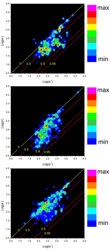
The first results we report in Fig. 1 show the 2-D histogram of e−_{versus e}+_{in Log-Log scale, being e}−_{and e}+_{the power}

associated to δz−and δz+ fluctuations, computed from the trace of the corresponding variance matrix of the compo-nents. These variances were discarded whenever the number of elements within each 1 h interval was less than 30% of the total number, i.e. less than 14. The three panels of this figure refer, from top to bottom, to results obtained for the fast wind observed at 0.29, 0.65 and 0.88 AU (Table 1), respectively. Moreover, the colored straight lines indicate constant values of σC. The distribution, which at 0.29 AU shows a well

de-fined single peak between 0.9 and 0.95 σC lines, becomes

less defined at 0.65 AU, shifts the main core of the distribu-tion towards smaller values of e+and starts to develop a tail towards much lower values of σC. This tendency becomes a

clear evidence at 0.88 AU when a second distribution is es-tablished along the σC∼0 line. This second family is located

above the main distribution and is due to enhanced values of e−rather than to depleted values of e+. If we try to estimate the number of values forming the upper distribution, choos-ing σC=0.5 as the border line between the two distributions,

we come out with a remarkable fraction of ∼30% of the total number of elements.

Because of its definition, σC=0H⇒e+=e− and, in turn, e+_=e−_{H⇒δv ⊥ δb, i.e. complete misalignment, or E}b or Ek=0. In order to understand the role played by magnetic

2.0 2.5 3.0 3.5 4.0 4.5 5.0 5.5 1.0 1.5 2.0 2.5 3.0 3.5 4.0 4.5 0.95 0.9 0.5 0 1.000 8.375 15.75 23.13 30.50 37.88 45.25 52.63 60.00 Log(e+ ) L o g (e -) 2.0 2.5 3.0 3.5 4.0 4.5 5.0 5.5 1.0 1.5 2.0 2.5 3.0 3.5 4.0 4.5 0.95 0.9 0.5 0 1.000 3.375 5.750 8.125 10.50 12.88 15.25 17.63 20.00 Log(e+) L o g (e -) 2.0 2.5 3.0 3.5 4.0 4.5 5.0 5.5 1.0 1.5 2.0 2.5 3.0 3.5 4.0 4.5

max

min

min

max

max

min

0. 0.5 0.95 0.9 1.000 2.750 4.500 6.250 8.000 9.750 11.50 13.25 15.00 Log(e+ ) L o g (e -)

Fig. 1. From top to bottom: frequency histograms of log(e−) ver-sus log(e+) for fast wind observed by Helios 2 at 0.29, 0.65 and 0.88 AU, respectively. The color code, for each panel, is normalized to the maximum of the distribution. Colored straight lines indicate constant values of σ_C.

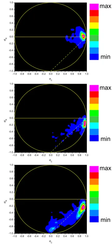
and kinetic energy in the previous distributions, we built a 2-D histogram of σR versus σC values for the same data

in--1.0 -0.8 -0.6 -0.4 -0.2 0.0 0.2 0.4 0.6 0.8 1.0 -1.0 -0.8 -0.6 -0.4 -0.2 0.0 0.2 0.4 0.6 0.8 1.0 2.000 25.50 49.00 72.50 96.00 119.5 143.0 166.5 190.0 σ C σ R -1.0 -0.8 -0.6 -0.4 -0.2 0.0 0.2 0.4 0.6 0.8 1.0 -1.0 -0.8 -0.6 -0.4 -0.2 0.0 0.2 0.4 0.6 0.8 1.0 1.000 6.500 12.00 17.50 23.00 28.50 34.00 39.50 45.00 σ C σ R -1.0 -0.8 -0.6 -0.4 -0.2 0.0 0.2 0.4 0.6 0.8 1.0 -1.0 -0.8 -0.6 -0.4 -0.2 0.0 0.2 0.4 0.6 0.8 1.0

max

min

min

max

min

max

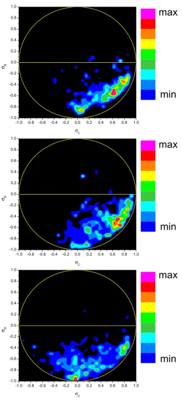
2.000 7.375 12.75 18.13 23.50 28.88 34.25 39.63 45.00 σ C σ R

Fig. 2. From top to bottom: frequency histograms of σR versus

σC for fast wind observed by Helios 2 at 0.29, 0.65 and 0.88 AU,

respectively. The color code, for each panel, is normalized to the maximum of the distribution. The yellow circle represents the lim-iting value given by σC2+σR2=1 while, the yellow dashed line

represents the relation σR=σC−1, see text for details. .

tervals analyzed in Fig. 1. These results, shown in Fig. 2, highlight the presence of a radial evolution of the fluctuations

towards a double-peaked distribution during the expansion of the wind. While at 0.3 AU the peak of the distribution, well centered around σR∼0 and σC∼1, suggests the

overwhelm-ing presence of outwardly propagatoverwhelm-ing Alfv´en modes, the distribution corresponding to 0.7 AU denotes the formation of a tail towards negative values of σR and lower values of σCwith a consequent depletion of the main peak with respect

to the whole distribution. Moreover, this peak loses some of the Alfv´enic character it showed in the previous panel since it is located at negative σR. This tendency ends up with

the appearance of a sort of secondary peak when the wind reaches 0.88 AU. This new born peak forms around σR∼−1

and σC∼0. These characteristics suggest that this new-born

family might be made of MFDT structures just like those found by Tu and Marsch (1991). Parallel to the appearance of these fluctuations, the main peak characterized by Alfv´en-like fluctuations moves to lower and lower values of σR and σC loosing much of the original character it had at 0.3 AU.

At this point, we can introduce a new limit on σRin order to

better identify those fluctuations which do not have Alfv´enic character and are characterized by a clear excess of magnetic energy. Thus, if we count all the intervals for which σC<0.5

and σR<−0.6 we end up with a population of about 23% of

the total number of intervals.

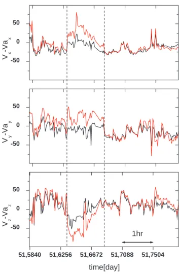
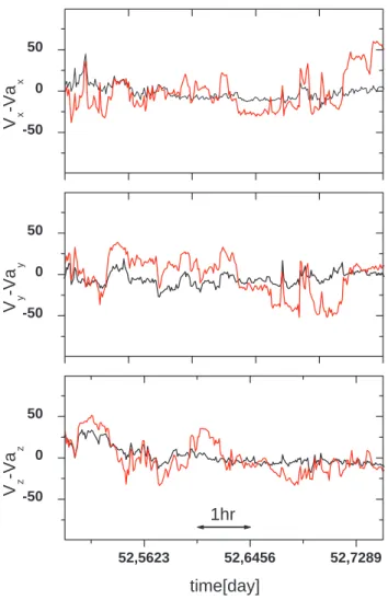
In the next Fig. 3 we take a look at one of these events located within the trailing edge of the high velocity stream observed at 0.88 AU. The three panels, from top to bottom, show the 81 s fluctuations of the three components of ve-locity (black solid line) and magnetic field (red solid line), expressed in Alfv´en units, relative to their respective aver-age values. The two vertical dashed lines highlight a sub-interval lasting more than 1 h during which magnetic fluc-tuations largely dominate over kinetic flucfluc-tuations. More-over, it is interesting to notice how this interval is located between two regions characterized by much better Alfv´enic correlations and energy equipartition. As a matter of fact, this central region shows also a higher level of variability in terms of magnetic field intensity, plasma density and temper-ature (not shown here) which would suggest a sort of pres-sure balance structure. Together with these relatively short intervals there are also much longer time intervals during which magnetic energy dominates and Alfv´enic correlation is very low. One of these intervals is shown in Fig. 4 and is taken from the trailing edge of the same high velocity stream previously discussed. This case differs from the one shown before mainly because it lasts several hours and closely re-sembles the events shown by Tu and Marsch (1991) that they called MFDTs.

Tu and Marsch (1991) made the hypothesis that fluctua-tions were made solely by Alfv´en waves outwardly propa-gating and advected MFDTs, and derived a simple expres-sion relating the Alfv´en ratio rA=Ek/Ebto σC

rA= σC/(2 − σC) -50 0 50 V x -Va x -50 0 50 V y -Va y 51,5840 51,6256 51,6672 51,7088 51,7504 -50 0 50 1hr time[day] V z -Va z

Fig. 3. From top to bottom: 81 s fluctuations of the three

com-ponents of velocity (black solid line) and magnetic field (red solid line), expressed in Alfv´en units, relative to their respective average values. This time interval belongs to the trailing edge of a high speed stream observed at 0.88 AU. Distance between two consecu-tive tick marks on the “X” axis corresponds to 1 h.

which, however, only qualitatively agreed with Helios ob-servations, as can be seen from their Fig. 8. This expres-sion, taking into account that the normalized residual energy σRcan be expressed in terms of rAas σR=(rA−1)/(rA+1),

would also bring the following linear relation between σRand σC(Bavassano et al., 1998):

σR= σC− 1 (2)

which would replace the canonical quadratic relation σ_R2_+σC2_{≤1 and would be satisfied by a magnetic field} vec-tor b=v+c where v is the velocity vecvec-tor and c an arbitrary vector ⊥ v and due to MFDTs. These magnetic fluctua-tions would then alter the b, v alignment due to the presence of outwardly propagating Alfv´enic fluctuations, reducing the value of σC. However, the yellow dashed line shown in the

-50 0 50 V x -Va x -50 0 50 V y -Va y 52,5623 52,6456 52,7289 -50 0 50 1hr time[day] V z -Va z

Fig. 4. From top to bottom: 81 s fluctuations of the three

compo-nents of velocity and magnetic field in the same format as of Fig. 3. Also this time interval belongs to the trailing edge of the same high speed stream.

to provide a satisfactory, quantitative fit to the distribution. This result confirms similar conclusions drawn by Tu and Marsch (1991) in their original analysis.

Another way to look at the same data is shown in Fig. 5 where the average value of σRcomputed for each square bin

log(e−_)×log(e+_{) is shown for the same three time intervals.}

The color code indicates that only fluctuations observed at the shortest heliocentric distance (top panel) are character-ized by values of σR close to equipartition between Eb and Ek. As the wind expands, σR becomes more and more

neg-ative although high values of σC around the 0.95 line are

still present even at 0.88 AU (bottom panel). Finally, the new population that clearly appears at 0.88 AU around σC∼0, is

totally characterized by values of σR∼−1, indicating that

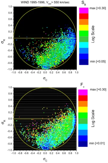
magnetic field fluctuations dominate the turbulent dynamics. At this point, it is interesting to look at the compressive level of these fluctuations as shown in Fig. 6. The up-per panel of Fig. 6 shows the histogram of magnetic field

2.0 2.5 3.0 3.5 4.0 4.5 5.0 5.5 1.0 1.5 2.0 2.5 3.0 3.5 4.0 4.5 0.95 0.9 0.5 0. σ R -1.000 -0.8625 -0.7250 -0.5875 -0.4500 -0.3125 -0.1750 -0.03750 0.1000 Log(e+₎ L o g (e -) 2.0 2.5 3.0 3.5 4.0 4.5 5.0 5.5 1.0 1.5 2.0 2.5 3.0 3.5 4.0 4.5 0.95 0.9 0.5 0. σ R -1.000 -0.8625 -0.7250 -0.5875 -0.4500 -0.3125 -0.1750 -0.03750 0.1000 Log(e+) L o g (e -) 2.0 2.5 3.0 3.5 4.0 4.5 5.0 5.5 1.0 1.5 2.0 2.5 3.0 3.5 4.0 4.5 0.95 0.9 0.5 0. σ R -1.000 -0.8625 -0.7250 -0.5875 -0.4500 -0.3125 -0.1750 -0.03750 0.1000 Log(e+₎ L o g (e -)

Fig. 5. From top to bottom: distribution of the average value of

σRcomputed within each square bin log(e−)×log(e+) for fast wind

observed by Helios 2 at 0.29, 0.65 and 0.88 AU, respectively. The color code, for each panel, indicates the interval value of σR.

compression defined as SB= q

σ_B2_/<|B|>2_{as a function of}

σR versus σC while, the lower panel shows the histogram

of FC=σB2/σxyz2 which measures the ratio of the variance of

-1.0 -0.8 -0.6 -0.4 -0.2 0.0 0.2 0.4 0.6 0.8 1.0 -1.0 -0.8 -0.6 -0.4 -0.2 0.0 0.2 0.4 0.6 0.8 1.0 L o g Sca le max [>0.3] min [<0.05] S_B 0.05000 0.06255 0.07825 0.09790 0.1225 0.1532 0.1917 0.2398 0.3000 σ C σ R -1.0 -0.8 -0.6 -0.4 -0.2 0.0 0.2 0.4 0.6 0.8 1.0 -1.0 -0.8 -0.6 -0.4 -0.2 0.0 0.2 0.4 0.6 0.8 1.0

Helios 2 at 0.88 AU within Fast Wind

L o g Sca le min [<0.01] max [>0.3] F_C 0.01000 0.01530 0.02340 0.03580 0.05477 0.08379 0.1282 0.1961 0.3000 σ C σ R

Fig. 6. From top to bottom: average value of SB and FC (see text

for definitions) computed within each square bin σR×σCfor Helios

2 observations at 0.88 AU within fast wind.

and σ_xyz2 the standard deviation of the magnetic field inten-sity and the trace of the variance matrix of the components, respectively (Bavassano et al., 1982a; Bruno and Bavassano, 1991). Both panels clearly indicate that the two regions char-acterized by σC∼1 and σR∼0 and σC∼0 and σR∼−1,

re-spectively, show the lowest magnetic compressive level. In particular, the lower panel indicates that most of the total vector variability is due to directional rather than compres-sive fluctuations, being this aspect, as already remarked in this paper, an intrinsic feature of Alfv´enic fluctuations and MFDTs. Thus these results would support the idea that these two populations would be due mainly to Alfv´enic outward fluctuations and MFDTs (Tu and Marsch, 1991, 1993), re-spectively. However, we cannot exclude that also Tangential Discontinuities, whose rate is expected to be at least one per hour (Tsurutani and Smith, 1979), might contribute to en-hance the imbalance in favor of magnetic energy.

0.5 1.0 1.5 2.0 2.5 3.0 3.5 4.0 4.5 0.5 1.0 1.5 2.0 2.5 3.0 3.5 4.0 4.5 0 0.5 0.9 0.95 1.000 1.625 2.250 2.875 3.500 4.125 4.750 5.375 6.000 Log(e+) L o g (e - ) 0.5 1.0 1.5 2.0 2.5 3.0 3.5 4.0 4.5 0.5 1.0 1.5 2.0 2.5 3.0 3.5 4.0 4.5 0.95 0. 0.9 0.5 1.000 1.875 2.750 3.625 4.500 5.375 6.250 7.125 8.000 Log(e+) L o g (e - ) 0.5 1.0 1.5 2.0 2.5 3.0 3.5 4.0 4.5 0.5 1.0 1.5 2.0 2.5 3.0 3.5 4.0 4.5

min

min

min

max

max

max

0 0.95 0.9 0.5 1.000 1.750 2.500 3.250 4.000 4.750 5.500 6.250 7.000 Log(e+) L o g (e - )

Fig. 7. From top to bottom: frequency histograms of log(e−) ver-sus log(e+) for slow wind observed by Helios 2 at 0.32, 0.69 and 0.90 AU, respectively. The color code, for each panel, is normalized to the maximum of the distribution.

Completely different is the situation within slow wind as shown in Fig. 7 where the 2-D histograms of log(e−) ver-sus log(e+) refer to the three intervals listed in Table 1. First of all, the distributions are quite spread and already

-1.0 -0.8 -0.6 -0.4 -0.2 0.0 0.2 0.4 0.6 0.8 1.0 -1.0 -0.8 -0.6 -0.4 -0.2 0.0 0.2 0.4 0.6 0.8 1.0 1.000 1.875 2.750 3.625 4.500 5.375 6.250 7.125 8.000 σ C σ R -1.0 -0.8 -0.6 -0.4 -0.2 0.0 0.2 0.4 0.6 0.8 1.0 -1.0 -0.8 -0.6 -0.4 -0.2 0.0 0.2 0.4 0.6 0.8 1.0 1.000 1.875 2.750 3.625 4.500 5.375 6.250 7.125 8.000 σ C σ R -1.0 -0.8 -0.6 -0.4 -0.2 0.0 0.2 0.4 0.6 0.8 1.0 -1.0 -0.8 -0.6 -0.4 -0.2 0.0 0.2 0.4 0.6 0.8 1.0

min

min

min

max

max

max

1.000 2.125 3.250 4.375 5.500 6.625 7.750 8.875 10.00 σ C σ R

Fig. 8. From top to bottom: frequency histograms of σR versus

σCfor slow wind observed by Helios 2 at 0.32, 0.69 and 0.90 AU,

respectively. The color code, for each panel, is normalized to the maximum of the distribution.

at 0.3 AU are not characterized by a single dominant peak as it was the case for fast wind. Moreover, the radial evo-lution is much less impressive than that for the fast wind. At 0.3 AU the main body of the distribution lies along the σC∼0.5 line and ends up at σC∼0 by the time the slow wind

reaches 0.88 AU. Consequently, also the σR-σC histograms

in Fig. 8 do not show a striking radial evolution. Although high values of σCcan be encountered also within slow wind

they are statistically much less relevant than in fast wind and a well defined population characterized by σC∼0 and σR∼−1, already present at 0.3 AU, becomes one of the

dom-inant peaks of the histogram when the wind reaches 0.88 AU. This last feature represents the most striking difference with what happens in fast wind. It is also worth noticing that, when the wind reaches 0.88 AU, some population with neg-ative σCclearly appears. However, the highly negative value

of the associated σR suggests that these elements cannot be

considered as inward propagating Alfv´en modes but rather as advected structures.

Figure 9, in the same format of Fig. 5, shows that highly negative values of σRare generalized and not exclusively

re-lated to any particular combination of e+ and e−, i.e. any particular value of σC, no matter what the heliocentric

dis-tance might be. On the other hand, values of σR close to 0

sporadically appear at all distances. This result confirms that in slow wind magnetic energy always dominates the fluctua-tions (see references in Bruno and Carbone, 2005) but rules out the possibility that this is solely due to an increased pres-ence of MFDTs (Tu and Marsch, 1993).

Finally, we like to underline that results, entirely similar to those shown so far in the present paper, have been obtained analyzing Helios 1 observations during its first solar mission in 1975 between 0.3 and 1 AU. However, we do not show them for sake of brevity.

2.2 WIND observations at 1 AU

To corroborate the results shown in the previous section with a more robust statistics, we employed WIND s/c data recorded for 14 months from the beginning of 1995 to day 121 of 1996. The data used in this analysis are 240 s averages of solar wind magnetic field and plasma. We removed all the magnetospheric crossings which represented about 7% of the selected time interval. The available number of 240 s aver-ages used for the analysis is then slightly more than 162 000. Proceeding like we did for Helios data, we computed the same quantities described in Sect. 2.1. During the time inter-val within which WIND’s data were analyzed, the solar wind was characterized mostly by corotating high velocity streams as expected for a typical minimum phase of the solar cycle (Bruno and Carbone, 2005). As suggested by Helios’ results in Sect. 2.1, we performed two analyses for fast and slow wind, separately (see Table 1 for details). For the fast wind we set up a lower speed limit of 550 km/s while, for the slow wind, we set up an upper speed limit of 400 km/s.

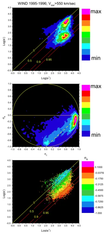
Results relative to fast wind are shown in Fig. 10 where, the top panel, shows the 2-D histogram for loge− and loge+ in the same format of Fig. 1, the lower panel shows the relative σR-σC histogram and the bottom panel shows

0.5 1.0 1.5 2.0 2.5 3.0 3.5 4.0 4.5 0.5 1.0 1.5 2.0 2.5 3.0 3.5 4.0 4.5 σ R σ R σ R 0.95 0.9 0.5 0. -1.000 -0.8625 -0.7250 -0.5875 -0.4500 -0.3125 -0.1750 -0.03750 0.1000 Log(e+ ) L o g (e -) 0.5 1.0 1.5 2.0 2.5 3.0 3.5 4.0 4.5 0.5 1.0 1.5 2.0 2.5 3.0 3.5 4.0 4.5 0.95 0.9 0.5 0. -1.000 -0.8625 -0.7250 -0.5875 -0.4500 -0.3125 -0.1750 -0.03750 0.1000 Log(e+ ) L o g (e -) 0.5 1.0 1.5 2.0 2.5 3.0 3.5 4.0 4.5 0.5 1.0 1.5 2.0 2.5 3.0 3.5 4.0 4.5 0.95 0.9 0.5 0. -1.000 -0.8625 -0.7250 -0.5875 -0.4500 -0.3125 -0.1750 -0.03750 0.1000 Log(e+ ) L o g (e -)

Fig. 9. From top to bottom: distribution of the average value of

σR computed within each square bin log(e−)×log(e+) for slow

wind observed by Helios 2 at 0.32, 0.69 and 0.90 AU, respectively. The color code, for each panel, indicates the interval value of σR.

log(e−_)×log(e+) in the same format of Fig. 5. Also in this case, as it already happened for the fast wind observed by He-lios at 0.88 AU, fluctuations appear to be divided into 2 main populations, namely Alfv´enic fluctuations and fluctuations

-1.0 -0.8 -0.6 -0.4 -0.2 0.0 0.2 0.4 0.6 0.8 1.0 -1.0 -0.8 -0.6 -0.4 -0.2 0.0 0.2 0.4 0.6 0.8 1.0 WIND 1995-1996; V_SW>550 km/sec 1.500 10.06 18.63 27.19 35.75 44.31 52.88 61.44 70.00 σ C σ R -0.5 0.0 0.5 1.0 1.5 2.0 2.5 3.0 3.5 4.0 4.5 -0.5 0.0 0.5 1.0 1.5 2.0 2.5 3.0 3.5 4.0 4.5 0 0.5 _0.9 0.95 1.500 10.06 18.63 27.19 35.75 44.31 52.88 61.44 70.00 Log(e+) L o g (e - ) -0.5 0.0 0.5 1.0 1.5 2.0 2.5 3.0 3.5 4.0 4.5 -0.5 0.0 0.5 1.0 1.5 2.0 2.5 3.0 3.5 4.0 4.5

max

max

min

min

0.95 0.9 0 0.5 σ R -1.000 -0.8625 -0.7250 -0.5875 -0.4500 -0.3125 -0.1750 -0.03750 0.1000 Log(e+) L o g (e - )

Fig. 10. Fast wind, with speed larger than 550 km/s, observed by

WIND s/c during 1995 and the first 4 months of 1996. From top to bottom: frequency histograms of log(e−) versus log(e+), fre-quency histograms of σR versus σC, distribution of the average

value of σR computed within each square bin log(e−)×log(e+),

respectively.

magnetically dominated. In order to evaluate the relevance of this second population we can adopt the same limits for

-0.5 0.0 0.5 1.0 1.5 2.0 2.5 3.0 3.5 4.0 4.5 -0.5 0.0 0.5 1.0 1.5 2.0 2.5 3.0 3.5 4.0 4.5 0 _0.5 0.9 0.95 1.200 26.05 50.90 75.75 100.6 125.4 150.3 175.1 200.0 Log(e+ ) L o g (e -) -1.0 -0.8 -0.6 -0.4 -0.2 0.0 0.2 0.4 0.6 0.8 1.0 -1.0 -0.8 -0.6 -0.4 -0.2 0.0 0.2 0.4 0.6 0.8 1.0

max

min

min

max

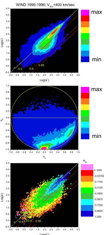
WIND 1995-1996; V_SW<400 km/sec 1.500 18.81 36.13 53.44 70.75 88.06 105.4 122.7 140.0 σ C σR -0.5 0.0 0.5 1.0 1.5 2.0 2.5 3.0 3.5 4.0 4.5 -0.5 0.0 0.5 1.0 1.5 2.0 2.5 3.0 3.5 4.0 4.5 0.95 0.9 0.5 0 σ R -1.000 -0.8625 -0.7250 -0.5875 -0.4500 -0.3125 -0.1750 -0.03750 0.1000 Log(e+) L o g (e -)

Fig. 11. Same format as of Fig. 10 but referring to slow wind, with

speed less than 400 km/s.

σC and σR that we used for Helios observations at 0.88 AU

within fast wind and we end up with a rough estimate around 25% of the total number, not far from the rough estimate we made in Sect. 2.1. Finally, it is worth noticing that the distri-bution shown in the middle panel has a sort of ridge which is well fitted by the yellow dashed line referring to Eq. (2). This

suggests that in some cases the simple model proposed by Tu and Marsch (1993) could be able to reproduce the observed situation to a good level and deserves some more careful and extensive analysis which cannot be done in this paper.

Next Fig. 11, in the same format of Fig. 10, shows the re-sults obtained for the slow wind, i.e. solar wind speed lower than 400 km/s. The distribution in the top panel is dominated by an elongated peak centered around σC=0 but located at

high values of e− and e+. Moreover, the same distribu-tion shows a bulge extending towards higher values of σC.

The lower panel clearly shows that the highest peak of the distribution belongs to a family characterized by σC≃0 and σR≃−1. On the other hand, the Alfv´enic population, which

dominates the fast wind, has almost disappeared. However, the bottom panel clearly suggests that those events strongly dominated by magnetic energy are mainly due to the largest values of e−_{and e}+_{as indicated by the color code. Also in}

this case, similarly to what we found for Helios 2 within fast wind (see Fig. 6) studying the compressive character of the fluctuations, WIND observations reveal that the lowest level of magnetic compression corresponds to those two popula-tions that we identifies as Alfv´enic fluctuapopula-tions and magnet-ically dominated events (Fig. 12). In particular, the general level of compression appears larger than in the Helios 2 be-cause our selection of WIND’s time intervals was done auto-matically after we set up a threshold in the speed and, con-sequently, some intervals belonging to stream-stream inter-face or other compressive regions might have been included. However, also in this case, the lower panel indicates that most of the total vector variability is due to directional rather than compressive fluctuations.

2.3 Ulysses observations out of the ecliptic

A further confirmation of the existence of two dominat-ing distinct families of MHD fluctuations in the solar wind comes from Ulysses observations at high latitude. As a mat-ter of fact, these observations, together with those relative to the ecliptic, provide a complete picture in the 3-D helio-sphere. The time period we chose for Ulysses spans from day 190 to day 330 of 1994. During this period of time the radial distance of the s/c was between 2.75 and 1.77 AU, the heliographic latitude varied between −72◦and −62◦with a maximum excursion at −80◦and the s/c was constantly im-mersed in a high velocity wind flowing at an average speed of ∼745 km/s (see Table 1). The data set consists of 8 min averages of magnetic field and velocity measurements. This analysis follows the steps of the analysis made by Bavassano et al. (1998) but it is limited to fast polar wind observed at the highest negative latitudes, choosing an interval of time similar to that analyzed by Bavassano et al. (2005) who se-lected the three southernmost solar rotation seen by Ulysses in 1994.

Figure 13, relative to Ulysses observations, not only con-firms previous results (Bavassano et al., 1998) but it also

-1.0 -0.8 -0.6 -0.4 -0.2 0.0 0.2 0.4 0.6 0.8 1.0 -1.0 -0.8 -0.6 -0.4 -0.2 0.0 0.2 0.4 0.6 0.8 1.0 L o g Sca le min [<0.01] max [>0.30] F_c 0.01000 0.01530 0.02340 0.03580 0.05477 0.08379 0.1282 0.1961 0.3000 σ C σ R -1.0 -0.8 -0.6 -0.4 -0.2 0.0 0.2 0.4 0.6 0.8 1.0 -1.0 -0.8 -0.6 -0.4 -0.2 0.0 0.2 0.4 0.6 0.8 1.0 L o g Sca le max [>0.30] min [<0.05] WIND 1995-1996, V_SW> 550 km/sec S B 0.05000 0.06255 0.07825 0.09790 0.1225 0.1532 0.1917 0.2398 0.3000 σ C σ R

Fig. 12. From top to bottom: average value of SBand FC(see text

for definitions) computed within each square bin σR×σCfor WIND

observations within fast wind, respectively.

strengthens the results we just obtained from Helios 2 and WIND observations. The top panel of this figure highlights again the presence of two main populations. One located close to σC=0 line and the other one at higher values of σC.

The lower two panels help to disclose the nature of these two different families which are, again, magnetically dominated and Alfv´enic fluctuations. These results resemble much more those obtained from Helios 2 at 0.88 AU and WIND at 1 AU rather than those relative to Helios 2 at 0.3 AU indicating that polar fast wind at roughly 2 AU is more evolved than ecliptic fast wind around 0.3 AU, as abundantly discussed in liter-ature (see review by Bruno and Carbone, 2005, and paper by Matthaeus et al., 1998). However, it should also be re-marked that the Alfv´enic peak of the distribution is character-ized by a larger negative value of σRwith respect to Helios 2

at 0.88 AU and WIND at 1 AU. At first sight, this feature might be attributed to the fact that, in this case, as generally done in literature (Bruno and Carbone, 2005), the pressure anisotropy factor F , contained in the conversion factor used

-1.0 -0.8 -0.6 -0.4 -0.2 0.0 0.2 0.4 0.6 0.8 1.0 -1.0 -0.8 -0.6 -0.4 -0.2 0.0 0.2 0.4 0.6 0.8 1.0

min

max

1.200 7.925 14.65 21.38 28.10 34.83 41.55 48.28 55.00 σ C σR 0.5 1.0 1.5 2.0 2.5 3.0 3.5 4.0 4.5 0.5 1.0 1.5 2.0 2.5 3.0 3.5 4.0 4.5 _σ R 0.95 0.9 0.5 0 -1.000 -0.8625 -0.7250 -0.5875 -0.4500 -0.3125 -0.1750 -0.03750 0.1000 Log[e+ ] L o g [e -] 0.5 1.0 1.5 2.0 2.5 3.0 3.5 4.0 4.5 0.5 1.0 1.5 2.0 2.5 3.0 3.5 4.0 4.5

max

min

Ulysses: day 190 to 330 of 1994 0.95 0.9 0.5 0 1.200 18.55 35.90 53.25 70.60 87.95 105.3 122.7 140.0 Log[e+ ] L o g [e -]

Fig. 13. Polar wind observed by Ulysses s/c during the south

pas-sage of 1994. From top to bottom: frequency histograms of log(e−) versus log(e+), frequency histograms of σR versus σC,

distribu-tion of the average value of σR computed within each square bin

log(e−_)×log(e+), respectively.

to transform magnetic into velocity fluctuations (Belcher and Davis Jr., 1971), i.e. v=(±F /√4πρ)b, is considered equal to 1. However, this fact has already been noticed and largely

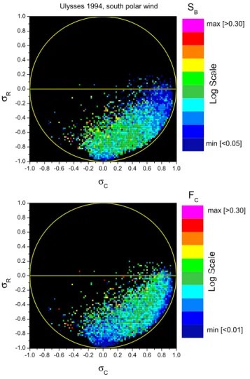
-1.0 -0.8 -0.6 -0.4 -0.2 0.0 0.2 0.4 0.6 0.8 1.0 -1.0 -0.8 -0.6 -0.4 -0.2 0.0 0.2 0.4 0.6 0.8 1.0 L o g Sca le L o g Sca le min [<0.05] max [>0.30] Ulysses 1994, south polar wind _S

B 0.05000 0.06255 0.07825 0.09790 0.1225 0.1532 0.1917 0.2398 0.3000 σ C σ R -1.0 -0.8 -0.6 -0.4 -0.2 0.0 0.2 0.4 0.6 0.8 1.0 -1.0 -0.8 -0.6 -0.4 -0.2 0.0 0.2 0.4 0.6 0.8 1.0 min [<0.01] max [>0.30] F C 0.01000 0.01530 0.02340 0.03580 0.05477 0.08379 0.1282 0.1961 0.3000 σ C σ R

Fig. 14. From top to bottom: average value of SB and FC (see

text for definitions) computed within each square bin σR×σCfor

Ulysses observations within the south polar wind, respectively. .

discussed by Bavassano and Bruno (2000) who accurately considered all effects due to total mass density, total ther-mal anisotropy, and ion differential streaming for a plasma made of protons, alpha particles and electrons. Their re-sults clearly indicated that, in the inner heliosphere, the ra-dial variation of the Alfv´en ratio rAtowards values less than

1 (i.e. σR<0) is not completely due to a missed inclusion

of multi-fluid effects in the conversion from magnetic field to Alfv´en units. On the other hand, Goldstein et al. (1995), discussing Ulysses results, suggested that the factor F in the Alfv´en relation might be sensitive to interstellar pick-up ions. As a matter of fact, these ions might appreciably influence the pressure anisotropy and, consequently, using F =1, as usually done in literature, would enhance the power asso-ciated to magnetic field fluctuations. Thus, this effect, dis-regardable in the inner heliosphere, might play a role in the case of Ulysses. Several other hypotheses have been formu-lated in literature to explain the radial behaviour of rA and

we invite the reader to take a look at the references related

to this topic and reported in the review by Bruno and Car-bone (2005). Thus, if pick-up ions play a significant role in case of Ulysses, we might ascribe to this phenomenon the fact that the yellow dashed line, which represents the Tu and Marsch (1991) model, completely misses the Alfv´enic pop-ulation. However, we also believe that the linear superpo-sition of Alfv´enic fluctuations and MFDTs, represented by relation (2), is not generally encountered in the solar wind and is an oversimplification of the real situation.

At this point we can attempt an estimate of the relative number of magnetic structures with respect to the whole data set. Adopting the same procedure used in the previous Sects. 2.1 and 2.2, that means counting only those elements with σC<0.5 and σR<−0.6, we end up with a population

of 27% of the total number, again, of the same order of the rough estimates we made for Helios 2 and WIND.

Finally, the two panels of Fig. 14, in the same format of Figs. 12 and 6, confirm that, also for Ulysses in the polar wind, the two main populations found by the present analy-sis are scarsely compressive as expected for Alfv´enic fluctu-ations and MFDTs (Tu and Marsch, 1991, 1993).

One more step towards the characterization of these mag-netic structures would be that of investigating how these events are distributed in time. If they were independent on each other we would expect to find a Poissonian distribution of the waiting times but, if some long range correlations ex-isted we would find a power-law like distribution (Bruno and Carbone, 2005). Keeping the limits for σC and σR that we

used to locate these events, we measured the time elapsed, i.e. the waiting time (WT, herefater), between the end of one event and the beginning of the next one. Obviously, the du-ration of each event is determined by the number of averages during which σC<0.5 and σR<−0.6. We performed this

kind of analysis only for Ulysses data set because of more robust statistics with respect to Helios 2 and because of a better continuity in the data coverage with respect to WIND (see Sect. 2.2).

The distribution of the normalized frequency of the WTs, expressed in minutes, is shown in Fig. 15. This distribution is clearly neither a power nor an exponential as demonstrated by the blue solid line representing the best possible fit ob-tained using a Poissonian curve y=(B/λ)e−λt_.

On the contrary, a distribution like

y = Axαe−tct ₍₃₎

which takes into account both contributions, i.e. the power law and the Poissonian, does a very good job as indi-cated by the solid red line. This fact suggests that the shortest magnetic structures keep a sort of memory of each other and that this long range correlation fades away as we look at events of this kind separated by longer and longer time intervals. Just for sake of complete-ness, we report the values obtained from the fitting proce-dure: A=49.05±9.13, α=−1.04±0.05, tc=412.05±62.54.

In particular, the value of the cutoff time tc indicates that

long term correlations loose strength for intervals longer than about 7 h.

3 Conclusions

The present analysis showed that magnetically dominated structures represent a remarkable component of the inter-planetary MHD fluctuations. In fact, these structures and Alfv´enic fluctuations dominate at scales typical of MHD tur-bulence. A rough estimate would suggest that more than 20% of all analyzed intervals of 1 h scale are magnetically domi-nated and weakly Alfv´enic. Observations in the ecliptic and out of the ecliptic showed that these advected, mostly un-compressive structures are ubiquitous in the heliosphere and can be found in both fast and slow wind. On the contrary, the same analysis confirmed that Alfv´enic fluctuations outwardly propagating strongly characterize fast wind but are rather negligible in slow wind, as we already know from literature (see review by Bruno and Carbone, 2005). In particular, He-lios 2 and HeHe-lios 1 (results from the latter s/c have not been shown in the present paper for sake of brevity) observations revealed a clear radial dependence of these magnetic struc-tures within fast wind, but not within slow wind. At short heliocentric distances (∼0.3 AU) the turbulent population is largely dominated by Alfv´enic fluctuations characterized by high values of σC and a rather good level of energy

equipar-tition (σR∼0). However, as the wind expands, a new-born

population, characterized by lower values of σC and higher

negative values of σR becomes visible. Helios observations

show that a new peak, located at σC∼0 and σR∼−1, clearly

appears in the distributionby the time the s/c reaches 1 AU. As a matter of fact, results from the analysis of Ulysses’ fast polar wind and WIND’s fast wind well resemble and cor-roborate Helios results obtained in proximity of 1 AU. More-over, we showed that, within fast wind, these magnetic struc-tures well mimic e− modes as it was stressed by Tu and Marsch (1991, 1993) in the case of MFDTs. As a matter of fact, most of the magnetic structures that we find share similar features with the MFDTs described by these authors although we cannot exclude that contributions to lower val-ues of σRmight also come from simple Tangential

Disconti-nuities which are ubiquitous in the solar wind.

Now, the question is whether or not these structures are created during the turbulent evolution of the fluctuations or they are already there at 0.3 AU but too small compared to Alfv´enic fluctuations to be seen. The fact that they are al-ways present within slow wind already at 0.3 AU, where Alfv´enic fluctuations are rather small, make us favor the so-lar origin of these structures. The reason why we do not see them at 0.3 AU is due to the fact that these fluctuations, mainly non-compressive, change the direction of the mag-netic field similarly to Alfv´enic fluctuations but producing a much smaller effect. As the wind expands, the Alfv´enic

102 103 10-3 10-2 10-1 100 y=axαe(-x/xc) y=(b/λ_)e(-x/λ)

Ulysses waiting time statistics for MFDTs

N

o

rma

lize

d

F

re

q

u

e

n

cy

Minutes

Fig. 15. Waiting time statistics for MFDTs events (see text for

selec-tion criteria) observed by Ulysses. Frequency has been normalized to the total number of events. The blue and red curves are the best fits to the data, obtained using the relative expressions listed in the inset.

component undergoes non-linear interactions which produce a transfer of energy to smaller and smaller scales while, these structures, being advected, have a much longer lifetime. As the expansion goes on, the relative weight of these fluctu-ations grows and they start to be detected in our analysis. To this regard, Tu and Marsch (1992) and Tu and Marsch (1993) suggested that large scale variations along the mag-netic field lines might be intermingled with small scale vari-ations perpendicular to these lines, being the former static structures advected by the wind and the latter Alfv´enic fluc-tuations. Depending on the relative direction in which the ob-server samples the solar wind parameters with respect to the background magnetic field a different mixture of Alfv´enic fluctuations and static structures will contribute to the re-sulting value of σC and σR. This angular effect would be

more and more important with increasing heliocentric dis-tance because of the spiral configuration of the interplanetary

magnetic field and of the larger radial damping of Alfv´enic fluctuations compared to advected structures. These struc-tures would represent a specific kind of the 2-D turbulence (Tu and Marsch, 1993) reported by Matthaeus et al. (1990). Following (Tu and Marsch, 1993), MFDTs would arise natu-rally like the Alfv´enic fluctuations since they obey the MHD equations because of the following properties: B·∇B=0 and V , |B|, ρ all constant (Tu and Marsch, 1991). While at short heliocentric distances 2-D turbulence might be of the stan-dard type since B0≫δb, MFDTs could be the final state of a

radial fast evolution experienced by these fluctuations within the first layers of the solar corona (Tu and Marsch, 1993).

Interesting enough is the the theoretical model presented by Chang et al. (2004) which tells us that propagating modes and coherent, advected structures are both necessary, insepa-rable ingredients of MHD turbulence, since they share a com-mon origin within the general view described by the physics of complexity (Chang, 2003; Chang et al., 2004). Propagat-ing modes experience resonances which generate coherent structures which, in turn, will migrate, interact and eventu-ally generate new modes.

Our interpretation is that at least part of these magnetic structures might also be a specific, uncompressive, signa-ture of the crossing of the border between adjacent flux tubes forming, as suggested by Bruno et al. (2001); Bruno et al. (2004); Bruno and Carbone (2005), the advected background structure of the interplanetary magnetic field, strongly related to the complex magnetic topology at the sun’s surface. How-ever, a more specific study is needed to prove our interpre-tation since these structures may not necessarily occur near the border of a stream tube, as remarked by Tu and Marsch (1991). Finally, we like to recall that the waiting time statis-tics elaborated for Ulysses observations showed that these structures might hide some long-range correlation, i.e. a sort of “memory”, which would make the underlying generating process non-Poissonian, possibly a cascading process.

Whatever the nature of these fluctuations might be, we showed that they represent a remarkable fraction of all fluc-tuations. Our statistical study provides a rough estimate of the importance of magnetically dominated structures in the solar wind turbulence.

Acknowledgements. Helios 2 magnetic field 81 s averages derive

from the Rome-GSFC magnetic experiment (P. I. S. F. Mariani and N. F. Ness). Plasma data form the same s/c derive from the solar wind analyzer and were provided by H. Rosenbauer and R. Schwenn, PIs of the experiment. The use of data of the so-lar wind plasma analyzer (P. I. D. J. McComas, Southwest Re-search Institute, San Antonio, Texas, USA) and of the magnetome-ters (P. I. A. Balogh) aboard the Ulysses spacecraft is gratefully ac-knowledged. We also acknowledge the use of data of the solar wind plasma analyzer (P. I. K. Ogilvie, NASA-GSFC, MD, USA) and of the magnetometers (P. I. R. Lepping) aboard the WIND spacecraft The data have been made available by the World Data Center A for Rockets and Satellites (NASA/GSFC, Greenbelt, Maryland, USA). We also thank E. Pietropaolo for computer assistance. The present

work has been supported by the Italian Space Agency (ASI) under contract #035/05/0.

Topical Editor B. Forsyth thanks M. Goldstein and S. Oughton for their help in evaluating this paper.

References

Bavassano, B. and Bruno, R.: Velocity and magnetic field fluctu-ations in Alfvnic regions of the inner solar wind: Three-fluid observations, J. Geophys. Res., 105, 5113–5118, 2000.

Bavassano, B., Dobrowolny, M., Fanfoni, G., Mariani, F., and Ness, N.: Statistical properties of MHD fluctuations associated with high-speed streams from Helios 2 observations, Solar. Phys., 78, 373–384, 1982a.

Bavassano, B., Dobrowolny, M., Mariani, F., and Ness, N.: Radial evolution of power spectra of interplanetary Alfv´enic turbulence, J. Geophys. Res., 87, 3617–3622, 1982b.

Bavassano, B., Pietropaolo, E., and Bruno, R.: Cross-helicity and residual energy in solar wind turbulence. Radial evolution and latitudinal dependence in the region from 1 to 5 AU, J. Geophys. Res., 103, 6521–6530, 1998.

Bavassano, B., Pietropaolo, E., and Bruno, R.: Alfv´enic turbu-lence in the polar wind: A statistical study on cross helicity and residual energy variations, J. Geophys. Res., 105, 12 697–12 704, 2000.

Bavassano, B., Bruno, R., and D’Amicis, R.: Large-scale velocity fluctuations in polar solar wind, Ann. Geophys., 23, 1025–1031, 2005,

http://www.ann-geophys.net/23/1025/2005/.

Belcher, J. and Davis Jr., L.: Large-amplitude Alfv´en waves in the interplanetary medium, J. Geophys. Res., 76, 3534–3563, 1971. Bieber, J., Wanner, W., and Matthaeus, W.: Dominant

two-dimensional solar wind turbulence with implications for cosmic ray transport, J. Geophys. Res., 101, 2511–2522, 1996. Bruno, R. and Bavassano, B.: Origin of low cross-helicity regions

in the solar wind, J. Geophys. Res., 96, 7841–7851, 1991. Bruno, R. and Bavassano, B.: Cross-helicity depletions in the inner

heliosphere, and magnetic field and velocity fluctuation decou-pling, Planet. Space Sci., 41, 677–685, 1993.

Bruno, R. and Carbone, V.: The Solar Wind as a Turbulence Labo-ratory, Living Reviews in Solar Physics, 2, 2005.

Bruno, R., Carbone, V., Veltri, P., Pietropaolo, E., and Bavassano, B.: Identifying intermittent events in the solar wind, Planetary Space Sci., 49, 1201–1210, 2001.

Bruno, R., Carbone, V., Primavera, L., Malara, F., Sorriso-Valvo, L., Bavassano, B., and Veltri, P.: On the probability distribution function of small-scale interplanetary magnetic field fluctuations, J. Geophys. Res., 22, 3751–3769, 2004.

Chang, T.: Complexity Induced Plasma Turbulence in Coronal Holes and the Solar Wind, in: AIP Conf. Proc. 679: Solar Wind Ten, edited by: Velli, M., Bruno, R., and Malara, F., pp. 481–484, 2003.

Chang, T., Tam, S., and Wu, C.: Complexity induced anisotropic bimodal intermittent turbulence in space plasmas, Phys. Plasmas, 11, 1287–1299, 2004.

Dobrowolny, M., Mangeney, A., and Veltri, P.: Properties of mag-netohydrodynamic turbulence in the solar wind, Astron. Astro-phys., 83, 26–32, 1980.

Els¨asser, W.: The hydromagnetic equations, Phys. Rev., 79, 183, 1950.

Goldstein, B. E., Neugebauer, M., and Smith, E. J.: Alfv´en waves, alpha particles, and pickup ions in the solar wind, Geophys. Res. Lett., 22, 3389–3392, doi:10.1029/95GL03182, 1995.

Goldstein, M., Roberts, D., and Matthaeus, W.: Systematic errors in determining the propagation direction of interplanetary Alfv´enic fluctuations, J. Geophys. Res., 91, 13 357–13 365, 1986. Grappin, R., Mangeney, A., and Marsch, E.: On the origin of

solar wind turbulence:Helios data revisited, in: Proceedings of the workshop on Turbulence and Non-linear Dynamics in MHD flows, edited by: Meneguzzi, M., Pouquet, A., and Sulem, P., pp. 81–86, North-Holland, 1989.

Horbury, T. S., Forman, M. A., and Oughton, S.: Spacecraft observations of solar wind turbulence: an overview, Plasma Physics and Controlled Fusion, 47, B703–B717, doi:10.1088/ 0741-3335/47/12B/S52, 2005.

Klein, L., Bruno, R., Bavassano, B., and Rosenbauer, H.: Anisotropy and minimum variance of magnetohydrodynamic fluctuations in the inner heliosphere, J. Geophys. Res., 98, 17 461–17 466, 1993.

Marsch, E. and Tu, C.-Y.: Dynamics of correlation functions with Els¨asser variables for inhomogeneous MHD turbulence, J. Plasma Phys., 41, 479–491, 1989.

Matthaeus, W., Goldstein, M., and Roberts, D.: Evidence for the presence of quasi-two-dimensional nearly incompressible fluctu-ations in the solar wind, J. Geophys. Res., 95, 20 673–20 683, 1990.

Matthaeus, W. H., Smith, C. W., and Oughton, S.: Dynamical age of solar wind turbulence in the outer heliosphere, J. Geophys. Res., 103, 6495–6502, 1998.

Montgomery, D.: Major disruptions, inverse cascades, and the Strauss equations, Phys. Scr., 2, 83–88, 1982.

M¨uller, W.-C. and Grappin, R.: Spectral Energy Dynamics in Mag-netohydrodynamic Turbulence, Phys. Rev. Lett., 95, 114 502– 114 505, 2005.

Oughton, S., Priest, E. R., and Matthaeus, W. H.: The influence of a mean magnetic field on three-dimensional magnetohydrody-namic turbulence, J. Fluid Mech., 280, 95–117, 1994.

Roberts, D.: Observation and simulation of the radial evolution and stream structure of solar wind turbulence, in: Solar Wind Seven Colloquium, pp. 533–538, 1992.

Roberts, D., Goldstein, M., Klein, L., and Matthaeus, W.: The na-ture and evolution of magnetohydrodynamic fluctuations in the solar wind: Voyager observations, J. Geophys. Res., 92, 11 021– 11 040, 1987a.

Roberts, D., Goldstein, M., Klein, L., and Matthaeus, W.: Origin and evolution of fluctuations in the solar wind: HELIOS obser-vations and Helios-Voyager comparisons, J. Geophys. Res., 92, 12 023–12 035, 1987b.

Roberts, D., Ghosh, S., Goldstein, M., and Matthaeus, W.: Mag-netohydrodynamic simulation of the radial evolution and stream structure of solar-wind turbulence, Phys. Rev. Lett., 67, 3741– 3744, 1991.

Roberts, D., Goldstein, M., Matthaeus, W., and Ghosh, S.: Velocity shear generation of solar wind turbulence, J. Geophys. Res., 97, 17 115–17 130, 1992.

Shebalin, J., Matthaeus, W., and Montgomery, D.: Anisotropy in MHD turbulence due to a mean magnetic field, J. Plasma Phys., 29, 525–547, 1983.

Smith, C.: The Geometry of Turbulent Magnetic Fluctuations at High Heliograpahic Latitudes, in: Solar Wind Ten, edited by: Velli, M., Bruno, R., and Malara, F., vol. 679 of AIP Conf. Proc., pp. 413–416, 2003.

Tsurutani, B. and Smith, E.: Interplanetary discontinuities: tempo-ral variations and the radial gradient from 1 to 8:5AU, J. Geo-phys. Res., 84, 2773–2787, 1979.

Tu, C., Roberts, D., and Goldstein, M.: Spectral evolution and cas-cade constant of solar wind Alfv´enic turbulence, J. Geophys. Res., 94, 13 575–13 578, 1989.

Tu, C.-Y. and Marsch, E.: Transfer equations for spectral densities of inhomogeneous MHD turbulence, J. Plasma Phys., 44, 103– 122, 1990.

Tu, C.-Y. and Marsch, E.: A case study of very low cross-helicity fluctuations in the solar wind, Ann. Geophys., 9, 319–332, 1991, http://www.ann-geophys.net/9/319/1991/.

Tu, C. Y. and Marsch, E.: The evolution of MHD turbulence in the solar wind, in: Solar Wind Seven Colloquium, pp. 549–554, 1992.

Tu, C.-Y. and Marsch, E.: A model of solar wind fluctuations with two components: Alfv´en waves and convective structures, J. Geophys. Res., 98, 1257–1276, 1993.

Tu, C.-Y. and Marsch, E.: MHD structures, waves and turbulence in the solar wind: Observations and theories, Space Sci. Rev., 73, 1–2, 1995.

Wanner, W. and Wibberenz, G.: A study of the propagation of solar energetic protons in the inner heliosphere, J. Geophys. Res., 98, 3513–3528, 1993.

Zank, G. and Matthaeus, W.: Waves and turbulence in the solar wind, J. Geophys. Res., 97, 17 189–17 194, 1992.

Zhou, Y. and Matthaeus, W.: Non-WKB evolution of solar wind fluctuations: A turbulence modeling approach, Geophys. Res. Lett., 16, 755–758, 1989.