HAL Id: hal-01625615
https://hal.archives-ouvertes.fr/hal-01625615
Submitted on 27 Oct 2017
HAL is a multi-disciplinary open access
archive for the deposit and dissemination of
sci-entific research documents, whether they are
pub-lished or not. The documents may come from
teaching and research institutions in France or
abroad, or from public or private research centers.
L’archive ouverte pluridisciplinaire HAL, est
destinée au dépôt et à la diffusion de documents
scientifiques de niveau recherche, publiés ou non,
émanant des établissements d’enseignement et de
recherche français ou étrangers, des laboratoires
publics ou privés.
fault networks: example for the western Corinth rift,
Greece
Thomas Chartier, Oona Scotti, Hélène Lyon-Caen, Aurélien Boiselet
To cite this version:
Thomas Chartier, Oona Scotti, Hélène Lyon-Caen, Aurélien Boiselet. Methodology for earthquake
rupture rate estimates of fault networks: example for the western Corinth rift, Greece. Natural
Hazards and Earth System Sciences, European Geosciences Union, 2017, 17 (10), pp.1857 - 1869.
�10.5194/nhess-17-1857-2017�. �hal-01625615�
https://doi.org/10.5194/nhess-17-1857-2017 © Author(s) 2017. This work is distributed under the Creative Commons Attribution 3.0 License.
Methodology for earthquake rupture rate estimates of fault
networks: example for the western Corinth rift, Greece
Thomas Chartier1,2, Oona Scotti2, Hélène Lyon-Caen1, and Aurélien Boiselet1,2,a
1Laboratoire de géologie, Ecole Normale Supérieure, CNRS UMR 8538, PSL Research University, Paris, 75005, France 2Bureau d’Evaluation des Risques Sismiques pour la Sûreté des Installations, Institut de Radioprotection
et de Sûreté Nucléaire, Fontenay-aux-Roses, France anow at: Axa Global P&C, Paris, 75008, France
Correspondence to:Thomas Chartier ([email protected]) Received: 30 March 2017 – Discussion started: 4 April 2017
Revised: 11 August 2017 – Accepted: 4 September 2017 – Published: 27 October 2017
Abstract. Modeling the seismic potential of active faults is a fundamental step of probabilistic seismic hazard assess-ment (PSHA). An accurate estimation of the rate of earth-quakes on the faults is necessary in order to obtain the prob-ability of exceedance of a given ground motion. Most PSHA studies consider faults as independent structures and neglect the possibility of multiple faults or fault segments rupturing simultaneously (fault-to-fault, FtF, ruptures). The Uniform California Earthquake Rupture Forecast version 3 (UCERF-3) model takes into account this possibility by considering a system-level approach rather than an individual-fault-level approach using the geological, seismological and geodetical information to invert the earthquake rates. In many places of the world seismological and geodetical information along fault networks is often not well constrained. There is there-fore a need to propose a methodology relying on geological information alone to compute earthquake rates of the faults in the network. In the proposed methodology, a simple distance criteria is used to define FtF ruptures and consider single faults or FtF ruptures as an aleatory uncertainty, similarly to UCERF-3. Rates of earthquakes on faults are then computed following two constraints: the magnitude frequency distribu-tion (MFD) of earthquakes in the fault system as a whole must follow an a priori chosen shape and the rate of earth-quakes on each fault is determined by the specific slip rate of each segment depending on the possible FtF ruptures. The modeled earthquake rates are then compared to the available independent data (geodetical, seismological and paleoseis-mological data) in order to weight different hypothesis ex-plored in a logic tree.
The methodology is tested on the western Corinth rift (WCR), Greece, where recent advancements have been made in the understanding of the geological slip rates of the com-plex network of normal faults which are accommodating the ∼ 15 mm yr−1 north–south extension. Modeling results show that geological, seismological and paleoseismological rates of earthquakes cannot be reconciled with only single-fault-rupture scenarios and require hypothesizing a large spectrum of possible FtF rupture sets. In order to fit the im-posed regional Gutenberg–Richter (GR) MFD target, some of the slip along certain faults needs to be accommodated either with interseismic creep or as post-seismic processes. Furthermore, computed individual faults’ MFDs differ de-pending on the position of each fault in the system and the possible FtF ruptures associated with the fault. Finally, a comparison of modeled earthquake rupture rates with those deduced from the regional and local earthquake catalog statistics and local paleoseismological data indicates a bet-ter fit with the FtF rupture set constructed with a distance criteria based on 5 km rather than 3 km, suggesting a high connectivity of faults in the WCR fault system.
1 Introduction
The goal of probabilistic seismic hazard assessment (PSHA) is to estimate the probability of exceeding various ground-motion levels at a site (or a map of sites) given the rates of all possible earthquakes. The first step of PSHA follow-ing a Cornell–McGuire approach (Cornell, 1968; McGuire, 1976) is the characterization of the seismic sources. For
re-gions where active faults have been identified and their slip rates are known, several methods have been proposed in or-der to calculate the rate of earthquakes occurring on these faults. The most commonly used methods consider faults as independent structures on which the strong earthquakes are located (e.g., SHARE project in Europe, Woessner et al., 2015; Yazdani et al., 2016, in Iran; TEM model in Taiwan, Wang et al., 2016). In these PSHA studies, a background seismicity will generate earthquakes up to a threshold mag-nitude (Mw) of 6.0 or 6.5, beyond which earthquakes are generated on the faults. The rate of earthquakes for these larger magnitudes is based on geological and paleoseismo-logical records, and the maximum magnitudes depend on the physical dimensions of the fault under consideration. In the resulting model, the rate of lower magnitudes is controlled by seismological information and the rate of stronger magni-tudes by geological information. In cases where large his-torical earthquakes are associated with multiple fault seg-ments, the individual fault segments described by the geol-ogists in the field are regrouped in a larger fault source and a mean slip rate is attributed to the fault source. A specific magnitude frequency distribution (MFD), often Gutenberg– Richter (GR) (Gutenberg and Richter, 1944) or characteris-tic earthquake (Wesnousky, 1986), describing the mean slip-rate-based earthquake rate on the fault is attributed to each fault source. This process requires simplifying fault com-plexity in terms of geometry and slip rate and does not allow complex ruptures that propagate from one fault source to an adjacent one.
In the past decades, the quality of observations has im-proved and our understanding of earthquakes has grown (pro-ceedings of the 2017 Fault2SHA meeting). We observe more and more complex earthquake ruptures propagating on sev-eral neighboring faults. There is thus a need for hazard mod-els to accurately represent the fault and rupture complexity observed in the field by geologists and to correctly distin-guish aleatory from epistemic uncertainties.
Toro et al. (1997) define epistemic uncertainty as “uncer-tainty that is due to incomplete knowledge and data about the physics of the earthquake process. In principle, epistemic uncertainty can be reduced by the collection of additional information”. Aleatory uncertainty, on the other hand, is an “uncertainty that is inherent to the unpredictable nature of future events”; in this respect a fault-to-fault (FtF) rupture should be treated as an aleatory uncertainty since it is linked to the randomness of the seismic phenomenon.
In order to allow FtF ruptures, the Working Group on Cal-ifornia Earthquake Probabilities (WGCEP-2003) for the San Francisco Bay region developed a methodology that explores possible FtF ruptures in a logic tree. Each branch of the logic tree represents a seismic hazard model, and the rate of the corresponding FtF rupture scenario is obtained by weight-ing the branches. In the hazard study of the Marmara Re-gion in Turkey, Gulerce and Ocak (2013) used this approach and set the weight of each branch (or rupture scenario) such
that the mean seismicity rate modeled by the logic tree fits the recorded seismicity rate around the fault of interest. This method treats the uncertainty of FtF ruptures as an epistemic uncertainty in the PSHA calculation.
The Uniform California Earthquake Rupture Forecast ver-sion 3 (UCERF-3) model was developed using a novel methodology that treats all possible combinations of FtF rup-ture scenarios within the same branch of the logic tree as an aleatory uncertainty (Field et al., 2014). Per their terminol-ogy, faults are divided into smaller sections and all possible section-to-section ruptures are investigated. The possibility of ruptures happening is controlled by a set of geometric and physical rules and the rate of earthquakes is computed using a “grand inversion” of the seismological, geological, paleoseismological and geodetical data available in Califor-nia. The regional GR MFD of earthquakes of California and the geodetical deformation are used as a target for the total earthquake rupture forecast in each deformation model. This grand inversion relies also on estimates of the creep rate on faults deduced from local deformation data when available.
For many fault networks, only sparse seismological and geodetical data are available, and the geological record is often the most detailed source of information concerning the faults’ activity. In such cases, it is necessary to develop a methodology that allows building seismic hazard models relying only on geological data and yet allowing FtF ruptures as an aleatory uncertainty. The sparse geodetical, seismolog-ical and paleoseismologseismolog-ical data can then be used as a means of comparison to help weighting the different input hypothe-sis.
In this study we propose such a methodology based on the slip-rate budget of each fault, FtF ruptures hypothesis and assumptions on the shape of the MFD defined for the fault system as a whole. The methodology is developed so as to be flexible and applicable to regions where data on faults, geodesy and seismicity may be sparse. The rate of earthquakes on faults computed using geological informa-tion (slip rates) and is then compared to other sources of information such as the regional and local earthquake cata-logs and the paleoseismic data in order to weight the different epistemic uncertainty explored in the logic tree. Moreover, it is also known that faults accommodate important amounts of slip in either post-seismic slip or in creep events (e.g., L’Aquilla earthquake 2009; Cheloni et al., 2014; Napa earth-quake 2014; Lienkaemper et al., 2016). These phenomena, called non-main-shock slip (NMS) later on, are integrated in the slip rates deduced from geological information and should not be converted into earthquake rates when comput-ing seismic hazard. The methodology presented in this study allows part of the geological slip rate to be considered as NMS slip rate.
We use this methodology to generate fault-based hazard models for the western Corinth rift (WCR), Greece, which has been studied for the past decade by the Corinth Rift Lab-oratory Working Group (CRL-WG) (Lyon-Caen et al., 2004;
Bernard et al., 2006; Lambotte et al., 2014). A large number of active faults have been identified in this area, and a con-sensus about their possible geometries and activity rates has been reached within the CRL-WG (Boiselet, 2014). We used this geologic information to test our modeling approach and explore different epistemic uncertainties in a logic tree. Fi-nally, we compared the modeled earthquake rates of each fault with seismological and paleoseismological data in or-der to weight the hypothesis in the logic tree.
2 Novel methodology for taking faults into account in PSHA
In most regions of the world the amount of data available to model faults in a PSHA study is often sparse and uncertain. However, the need to consider such data in PSHA is increas-ing, and the methods to properly incorporate the available geological information in the hazard models are still miss-ing. In this context, we propose building a methodology that allows considering all the available information on faults, al-lows setting rules to define FtF ruptures and considers single faults or FtF ruptures as an aleatory uncertainty.
Our iterative method allows converting the slip-rate budget of each individual fault rate of earthquakes by requiring that the resulting regional MFD of earthquakes in the whole fault system follows an imposed shape. The MFD shape of each individual fault will thus be a result of the iterative process and not an imposed parameter.
The proposed method is presented here in a nutshell and illustrated in Fig. 1.
1. The necessary input data include the following: – A definition of the 3-D geometry of the fault
sys-tem.
– An estimate of the geological slip rates of each in-dividual fault that determines the slip-rate budget of the fault.
2. Setting up the methodology requires the following: – Choosing suitable scaling laws to estimate the
max-imum magnitude each fault can host.
– Assuming the minimum magnitude of earthquakes possible on the faults (Mw5.0 in this study). – Hypothesizing FtF rupture scenarios based on some
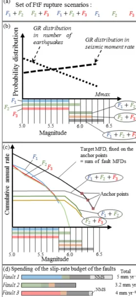
rules. In this study only a simple distance rule is used to define FtF ruptures. In future developments, more physics-based approaches could be explored. In the example presented in Fig. 1a, the three faults (fault 1, fault 2 and fault 3) are considered to be sufficiently close to each other; thus, they can either rupture individually (F1, F2, F3) or in FtF ruptures (F1 + F2, F2 + F3 or F1 + F2 + F3).
Figure 1. Illustration of the methodology. (a) Set of FtF rupture scenarios. (b) Picking of the magnitude bins and of the sources. (c) Building the target MFD: the black curve is the target MFD an-chored at the mean of the three highest magnitude bins (magnitude bin of 0.1). The sum of the resulting MFDs of the six sources has to be equal to the target MFD. (d) Visualization of the partitioning by the iterative methodology of each fault’s slip-rate budget (col-ors correspond to the individual rupture or the FtF rupture; NMS is non-main-shock slip).
– Imposing a shape for the target MFD for the whole fault system. In this study a GR MFD distribution is assumed.
3. Three pre-computational steps are performed to carry out the following:
– To calculate all possible magnitude bins each fault and FtF rupture scenario can accommodate accord-ing to each scalaccord-ing law considered (Fig. 1b).
– To calculate the number of incremental quantities of slip rate (dsr) contained in each fault budget. In the example, fault 1, fault 2 and fault 3 have a slip-rate budget of 5, 3.2 and 4 mm yr−1 respec-tively (Fig. 1d). Therefore, considering a dsr size of 0.01 mm yr−1, the faults budgets will be consumed after 500, 320 and 400 dsr respectively. The slip-rate budget of each fault may be spent along indi-vidual faults and/or FtF rupture scenarios.
– To convert the target MFD, expressed in terms of rate of earthquakes, into moment rates (Fig. 1b). This target MFD will be used to pick the magnitude bin on which an increment dsr will be spent. Notice that the formulation in terms of moment rate im-plies that greater magnitudes are more likely to be picked.
4. Iterative process is described as follows:
– First, the bin of magnitude (of width 0.1) where a dsr will be spent is picked according to the target MFD for the whole fault system in terms of moment rate.
– Then, in this bin of magnitude Mi, a seismotectonic source Si (an individual fault or an FtF scenario) that can host this magnitude is picked randomly. The increment of moment rate d ˙M0for this source is calculated following Eq. (1), and the rate of earth-quakes increment dreis calculated using Eq. (2). d ˙M0=µ · A ·dsr (1) dre(Mi) =
d ˙M0 M0(Mi)
, (2)
where d ˙M0 is the increment of moment rate for the source Si, µ the shear modulus of the fault, A the area of the source, dsr the increment of slip rate spent, dre(Mi) the increment of the rate of magnitude Mi, and M0(Mi) the seismic moment of a moment magnitude Mwdefined by Hanks and Kanamori (1979):
Mw= 2
3log (M0) −10.7. (3) – At each iteration, the slip-rate budget of the faults participating in the scenario accommodating the earthquakes of the three highest magnitude bins (0.3 being the range of uncertainties in the scal-ing laws used to assess the maximum magnitude) is checked:
– If there is still a portion of the slip-rate budget to be spent, the drecalculated is added to the rate of earthquakes of magnitude Mi for the source Si.
– If one of the faults of the FtF rupture generat-ing the largest earthquake has exhausted its slip-rate budget, the final slip-rates of the highest mag-nitude earthquakes are reached. Then, knowing the shape of the imposed target MFD, the target rate at the fault system level for all magnitudes bins is known (Fig. 1c). At this stage, an addi-tional check is performed:
– if adding the drecalculated for magnitude Mi onto the source Si leads to the exceeding of the target MFD for this magnitude, then this dre is not added to the source Si and the in-crement dsr of this computation step is con-sidered as NMS slip;
– if adding the dre to the source Si does not lead to the exceeding of the target MFD, this dreis added to the source Si.
– The increment of slip rate dsr is then removed from the slip-rate budget of the fault or the faults in-volved in source Si.
– If the slip-rate budget of each fault is exhausted, the fault and the corresponding FtF rupture scenar-ios the fault is involved in are removed and cannot be picked anymore in subsequent iterations of the computation.
– These steps are repeated until all the slip-rate bud-gets of all the faults in the system are spent either on single-fault ruptures, FtF ruptures or NMS slips. The output of this process is an earthquake rupture rate for different magnitudes for each fault and FtF rupture scenario in the model, considered as aleatory uncertainty. We also record how the slip-rate budget of each fault is partitioned between the different FtF ruptures and how much NMS slip was needed on each fault in order to fit the target MFD shape (here GR MFD) with a given set of FtF rupture scenarios (Fig. 1d). In the example, fault 1 spends 43 % of its budget on single-fault ruptures (blue color), 7 % on F1 + F2 ruptures (dark green), 23 % on F1 + F2 + F3 ruptures (dark grey) and 27 % on the NMS slips (light grey). On the other hand, 100 % of the slip-rate budget of the slower moving fault (i.e., fault 2) is converted into earthquake rates (0 % NMS) and limits the rate of the largest magnitude earthquakes (F1 + F2 + F3) (see Supplement).
A simplified example of the application of this methodol-ogy based on only two faults is presented in the Supplement to this paper. This example illustrates step by step the way in which the proposed methodology allows the transformation of slip-rate budgets of faults into earthquake rates.
Post-processing then includes the following: – Exploring the epistemic uncertainties:
Many assumptions have to be made when setting up the methodology (scaling law, FtF rupture set, faults
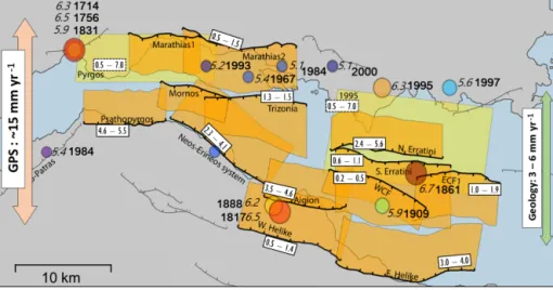
Figure 2. Map of the active faults of the western part of the Corinth rift (modified from Boiselet, 2014). The orange polygons are the surface projection of the active faults. The yellow polygons are the surface projection of the blind faults (Pyrgos fault and 1995 fault). Earthquakes of the catalog during the complete period are represented by circles with color and size depending on the magnitude. The date and magnitude of earthquake are indicated. The minimum and maximum values (mm yr−1) of the slip rates of the faults are indicated in the white boxes. The green arrow shows an approximation of the rift extension calculated by projecting horizontally the faults’ slip rate, and the pink arrow shows the extensional rate of the rift measured by GPS.
eters, etc.), and the different possible hypothesis should be explored in a logic tree.
– Reality checks:
The last step of the methodology involves comparing the modeled earthquake rates with independent data, such as the seismicity rates deduced from the catalog and paleoearthquake rates deduced from trench studies. Each branch of the logic tree is then weighted according to its performance with these independent data. In this study, we applied the proposed methodology to a well-documented rifting zone in the Aegean Sea (Fig. 2).
3 Application to the western Corinth rift fault system The east–west striking Corinth rift is the most seismically ac-tive structure in Europe with several earthquakes larger than Mw5.5 recorded in the historical times as well as in the in-strumental period (e.g., Jackson et al., 1982; Papazachos and Papazachou, 2003; Makropoulos et al., 2012). The Corinth Rift Laboratory was set up in 2001 in the western and most seismically active part of the rift (Lyon-Caen et al., 2004) with the goals of understanding the rifting process and pro-viding key elements for the seismic hazard assessment of the region.
The geodetical deformation measured by Global Posi-tioning System (GPS) shows a highly localized opening of the Corinth rift at a rate of 10 mm yr−1 in the east and 15 mm yr−1in the west (Avallone et al., 2004) over a width of less than 20 km, inducing a high strain rate. This deforma-tion is accommodated by a complex network of both
north-and south-dipping normal faults. Geological studies of these faults have shown that the north-dipping faults located on the southern coast have a higher slip rate than the south-dipping northern faults, giving the rift its asymmetrical structure. In the south, the Peloponnese is uplifted by the activity of these faults (Armijo et al., 1996; Ford et al., 2013), and in the north the coast line is subsiding.
The western Corinth rift fault slip rates were inferred from the displacement of geologic markers in the field or from seismic profiles on each individual fault, with the exception of the two blind faults identified by their recent seismic activ-ity (1995 fault, Bernard et al., 1997 and Pyrgos fault, Sokos et al., 2012) and for which the microseismicity recorded close to the fault was transformed into the slip rate on the fault plane. These latter slip rates are therefore subject to a very large uncertainty. The estimated geological extension rate expressed by the sum of the horizontal projection of the geological slip rates of the faults is in the range of 3 to 6 mm per year, which is three times less than the geodetical exten-sion rate. Given this disagreement, the WCR is a good candi-date to test whether the earthquake rates calculated using our methodology, which relies only on geological information, can account for the occurrence of the large earthquakes that have been documented in the region (Albini et al., 2017).
The WCR fault system has been described in detail by Boiselet (2014), who defined a model for the fault system, including geometries and slip rates for each fault (Fig. 2, Ta-ble 1) and a set of possiTa-ble FtF ruptures (hereafter model B14). The B14 model proposes a set of FtF rupture scenar-ios (Table 2) assuming that two neighboring faults can make up an FtF scenario only if they are less than 3 km apart. In
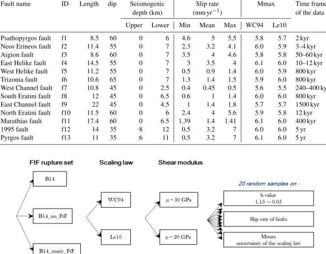
Table 1. Fault characteristics in Boiselet (2014). Mmax values calculated using the equations for normal faults using the rupture area. WC94 refers to Wells and Coppersmith (1994) and Le10 to Leonard (2010) scaling laws.
Fault name ID Length dip Seismogenic Slip rate Mmax Time frame depth (km) (mm yr−1) of the data Upper Lower Min Mean Max WC94 Le10
Psathopyrgos fault f1 8.5 60 0 6 4.6 5 5.5 5.8 5.7 2 kyr Neos Erineos fault f2 11.4 55 0 7 2.3 3.2 4.1 6.0 5.9 3–4 kyr Aigion fault f3 8.6 60 0 7 3.5 4 4.6 5.8 5.8 50–60 kyr East Helike fault f4 14.5 55 0 7 3 3.5 4 6.1 6.0 10–12 kyr West Helike fault f5 11.2 55 0 7 0.5 0.9 1.4 6.0 5.9 800 kyr Trizonia fault f6 10.6 65 0 7 1.3 1.4 1.5 5.9 6.0 800 kyr West Channel fault f7 10.8 45 0 2.5 0.4 0.45 0.5 5.6 5.5 240–400 kyr South Eratini fault f8 12 45 0 6.5 0.6 1 1.4 6.0 6.0 800 kyr East Channel fault f9 22 45 0 4.5 1 1.4 1.8 5.7 5.7 1500 kyr North Eratini fault f10 11.5 60 0 6 2.4 4 5.6 5.9 5.8 12 kyr Marathias fault f11 17.4 60 0 6.5 1.39 1.4 1.41 6.1 6.0 400 kyr 1995 fault f12 14 35 8 12 0.5 3.2 7 6.0 6.0 5 yr Pyrgos fault f13 11 35 6 11 0.5 3.2 7 6.1 6.0 5 yr
3 Figure 3. Logic tree explored for this study.
this paper, we also explore a logic tree branch for an alter-native rupture set (see Fig. 3) with higher fault connectivity (B14_hc), where faults can break together if their fault traces are separated by 5 km or less, therefore allowing a wider spectrum of possible FtF rupture scenarios (additional sce-narios in bold in Table 2). For a comparison with classical fault PSHA studies, we explore a branch with only a simple fault rupture called B14_s. In this branch no FtF rupture is allowed.
The target MFD is chosen to be in the shape of a GR MFD with a b value of 1.15 ± 0.05, which is a typical value for extensional systems (Schorlemmer et al., 2005).
In this study we explore other epistemic uncertainties having a potential impact on the modeled earthquake rates (Fig. 3) in addition to the different FtF rupture sets previ-ously described; two scaling laws (Wells and Coppersmith, 1994; Leonard, 2010) have been used to calculate the maxi-mum magnitude based on rupture area for normal faults, and two values of the shear modulus µ have been used: 30 GPa, a
commonly used value in hazard studies, and 20 GPa to repre-sent the low-shear wave velocity in the WCR region recently estimated based on ambient noise tomography (Giannopou-los et al., 2017). For each branch, 20 random samples are drawn from triangular distributions in order to explore the epistemic uncertainty affecting the b value of the target MFD (1.15 ± 0.05), the slip rate of the faults and the uncertainty within the scaling law.
4 Modeled earthquake rupture rates and comparison with independent data
Using our method, the modeled rate of earthquakes for the WCR is then compared to the rate of earthquakes observed in the catalog. The seismicity catalog considered in this study (Fig. 2) is the SHEEC catalog (Stucchi et al., 2012; Grün-thal et al., 2013) developed in the framework of the SHARE project updated for six historical earthquakes (Albini et al., 2017) and three instrumental earthquakes (based on Baker
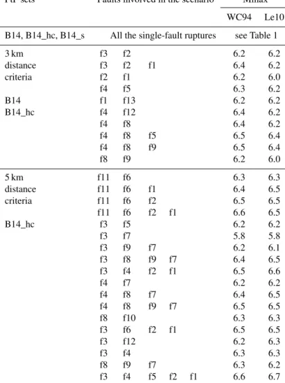
Table 2. Rupture scenarios considered in each model. Branch B14_s considers only the single-fault ruptures. Branch B14 considers the single-fault ruptures and the FtF ruptures with a 3 km distance criteria. Branch B14_hc considers the single-fault ruptures and the FtF ruptures with a 3 and a 5 km distance criteria. Mmax values are calculated using the equations for normal faults based on the rupture area. WC94: Wells and Coppersmith (1994); Le10: Leonard (2010).
FtF sets Faults involved in the scenario Mmax WC94 Le10 B14, B14_hc, B14_s All the single-fault ruptures see Table 1
3 km f3 f2 6.2 6.2 distance f3 f2 f1 6.4 6.2 criteria f2 f1 6.2 6.0 f4 f5 6.3 6.2 B14 f1 f13 6.2 6.2 B14_hc f4 f12 6.4 6.2 f4 f8 6.4 6.2 f4 f8 f5 6.5 6.4 f4 f8 f9 6.5 6.4 f8 f9 6.2 6.0 5 km f11 f6 6.3 6.3 distance f11 f6 f1 6.4 6.5 criteria f11 f6 f2 6.5 6.5 f11 f6 f2 f1 6.6 6.5 B14_hc f3 f5 6.2 6.2 f3 f7 5.8 5.8 f3 f9 f7 6.2 6.1 f3 f8 f9 f7 6.4 6.5 f3 f4 f2 f1 6.5 6.6 f4 f7 6.2 6.2 f4 f8 f7 6.4 6.5 f4 f8 f9 f7 6.5 6.5 f8 f10 6.3 6.3 f3 f6 f2 f1 6.5 6.5 f3 f12 6.2 6.3 f3 f4 6.3 6.3 f8 f9 f7 6.3 6.2 f3 f4 f5 f2 f1 6.6 6.7
et al., 1997; and P. Bernard from the 3HAZ Corinth project, personal communication, 2017). The updates and their im-plication on the catalog are summarized in Table 3. We prop-agate the earthquake magnitude uncertainties in the estimate of seismic moment rate and earthquake rate calculations by randomly sampling the magnitude of each earthquake within their uncertainties (Stucchi et al., 2012; Albini et al., 2017) and by using two hypotheses of completeness. In Table 4 the time of completeness of the catalog for Greece calculated by the SHARE project (Stucchi et al., 2012) and the times cal-culated by Boiselet (2014) using the approach proposed by Stepp (1972) at the scale of the Corinth rift region are re-ported.
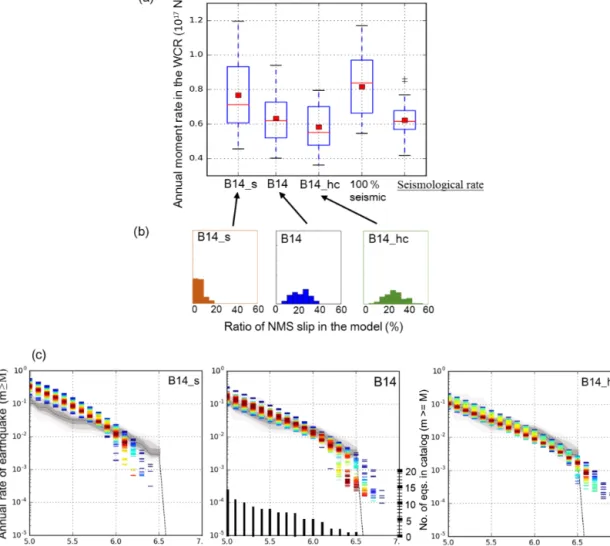
A first reality check is performed to compare the modeled and the catalog seismological moment rates. The seismologi-cal moment rate is seismologi-calculated directly using the rates of earth-quake of each magnitude in the catalog based on the moment
magnitude relation (Eq. 3) The seismic moment rates in mod-els B14 and B14_hc are in good agreement with the seismic moment rate deduced from the catalog, whereas B14_s pre-dicts a higher seismic moment rate (Fig. 4a). This compar-ison provides a better confidence in the models where FtF ruptures are possible than in the B14_s model. In the single-rupture model (B14_s), 90 % to nearly 100 % of the geologi-cal slip rate is converted into seismic moment rate with only less than 10 % interpreted as NMS slip rate. On the other hand, when FtF ruptures are possible (B14 and B14_hc), 25 % of the geological slip-rate budget of the faults is in-terpreted as NMS slip (Fig. 4b).
A second reality check consists in comparing modeled and catalog MFDs (Fig. 4c). The B14_s model does not manage to reproduce the rate of earthquakes deduced from the cat-alog, as it predicts a higher rate of Mw 5 earthquakes and no earthquakes of Mw 6.3 and above. On the other hand,
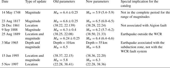
Table 3. Earthquakes updated in the historical and instrumental catalogs of the western Corinth rift.
Date Type of update Old parameters New parameters Special implication for the catalog
14 May 1748 Magnitude Mw=6.4 ± 0.25 Mw=5.9 (5.4–5.9) Not in the complete period for this
range of magnitudes 23 Aug 1817 Magnitude Mw=6.6 ± 0.25 Mw=6.5 (6.0–6.5)
26 Dec 1861 Location (38.22, 22.139) (38.28, 22.24) Not associated with Aigion fault 9 Sep 1888 Magnitude Mw=6.3 ± 0.4 Mw=6.2 (5.7–6.2)
25 Aug 1889 Location and magnitude
(38.25, 22.08) Mw=6.24 ± 0.25
(38.50, 21.33) Mw=6.4 (6.4–6.6)
Earthquake outside the WCR 3 Mar 1965 Depth and
magnitude
Depth = 10 km Mw=6.5
Depth = 55 km Mw=6.8
Earthquake associated with the subduction zone, not with the WCR fault system
15 Jun 1995 Location and magnitude (38.37, 22.15) Mw=5.8 (38.36, 22.20) Mw=6.3 5 Nov 1997 Location (22.28, 38.41) (22.28, 38.36)
we observe a good agreement of the MFDs of models B14 and B14_hc with the catalog. B14 reproduces the cumulative earthquake rate for Mw of 5.6 to 6.1 well, whereas model B14_hc reproduces the cumulative rate of earthquakes of Mw 5.0 to 5.5 better.
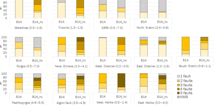
4.1 Slip-rate budget repartition
The way the slip-rate budget is spent between FtF ruptures, single-fault ruptures and the NMS slip ratio of the fault de-pends on the slip rate of the fault and the FtF ruptures the fault is involved in. Slow slipping faults that are involved in large FtF rupture scenarios (Neos Erineos or West Helike) have the majority of their slip-rate budget consumed by these large FtF ruptures (Fig. 5). On the contrary, the fast slipping faults that are involved in few FtF ruptures scenarios (1995, Pyrgos, North Eratini) spend their budget predominantly on single-fault ruptures producing a high number of small to medium magnitude earthquakes, which leads to easily ex-ceeding the GR regional target and thus implies a higher pro-portion of NMS slip rate on these faults.
Models B14 and B14_hc have a similar mean 25 % ratio of NMS slip ratio (Fig. 4), but this ratio is not distributed in the same way between the different faults in each model. However, an important NMS proportion on the blind faults (Pyrgos and 1995-fault) and the offshore North Eratini fault is found for both models. There are three main factors that can induce this result: either the FtF sets are not realistic, the slip rates explored on those faults are not realistic and do not include enough complex ruptures with these faults, or there is a mechanism of NMS slip such as creep or slow slip events happening on theses faults.
4.2 Earthquake rupture rate on the Aigion fault We now choose to focus our interest on the Aigion fault. Since this fault is one of the most active faults of the WCR
and crosses the city of Aigion, it represents a major source of seismic hazard and risk for the region.
The earthquake rate modeled on the Aigion fault depends of the FtF rupture set allowed in the model (Fig. 6). The resulting MFD of the Aigion fault has the shape of a GR MFD for model B14 and B14_s, with a steeper slope for the B14_s model. In the B14_hc, the MFD computed for the Ai-gion fault resembles a characteristic earthquake distribution of magnitude close to Mw6.0, similar to the maximum mag-nitude of earthquakes rupturing only the Aigion fault. It is worth noting that the larger magnitude earthquakes in Fig. 6b and c involve not only the Aigion fault but also the neighbor-ing faults participatneighbor-ing in the FtF ruptures (Fig. 5, Table 2).
Using the paleoseismological data presented by Pantosti et al. (2004), it is possible to propose rates of large magnitude earthquakes on the Aigion fault (Fig. 6). This paleorate (rate of paleoearthquakes) is subject to large uncertainties but can be used to validate or invalidate the different FtF rupture set hypothesis. In the B14_s model where faults only break on their own, the Aigion fault is not able to accommodate the paleoearthquake magnitudes. In the B14 model, where fault rupture is only allowed between faults separated by 3 km or less, the modeled earthquake rates are lower than the rates inferred from the paleoseismological study. In the B14_hc model, where FtF ruptures are allowed for faults separated by 5 km or less, the modeled earthquake rates agree well with the paleorate, within the margin of uncertainty.
According to the recent reappraisal of the historical seis-micity (Albini et al., 2017), the Aigion fault is most likely the source of the 1817 Mw 6.5 (6.0–6.5) and the 1888 Mw 6.2 (5.7–6.2) earthquakes. This leads to estimates of annual rates of Mw>6 earthquakes on the Aigion fault of 0.005 to 0.007 (Fig. 6) depending on the date of completeness of the catalog used (Table 4). The model B14_s does not manage to repro-duce the great magnitudes earthquakes observed in the cata-log. The annual rates for earthquakes Mw>6 of 0.0034 and
Figure 4. Modeled seismicity for the WCR fault network and comparison to the seismicity rate based on the earthquake catalog of the complete period. (a) Comparison between the modeled moment rates for each FtF scenario set and the seismological rate calculated from the earthquake catalog. Each box represents the SD around a mean and median value represented by a red square and a red line respectively. From left to right: the three first boxes are for each hypothesis scenario set in the logic tree, the fourth box shows the moment rate assuming 100 % of the slip rate of faults is converted into seismic moment, and the fifth box shows the moment rate calculated from the earthquake catalog. (b) Distribution of the ratio of NMS slip resulting from the three deformation models. (c) Comparison between the modeled GR MFD deduced from geological data for the whole fault system and that deduced from the WCR catalog. The models are represented as a colored density function with the red colors for the rates predicted by the higher number of models. The cumulative rates calculated from the catalog are shown as a grey density function. The cumulative number of earthquakes in the catalog is indicated by black bars in the central figure.
Table 4. Completeness hypothesis explored in this study. SHARE project Boiselet (2014) Magnitude Date of Magnitude Date of range completeness range completeness 4.1–5.1 1970 5.0–5.4 1958 5.1–5.7 1900 5.5–6.0 1904 5.7–6.5 1650 6.0–6.5 1725 ≥6.5 1450 6.5–7.0 1725
0.0051 predicted by models B14 and B14_hc respectively are statistically compatible with the rate inferred from the cata-log.
4.3 Weighting the logic tree branches
The comparison with independent local data allows sug-gesting weights for the different FtF rupture set hypothesis (Fig. 3) for hazard calculation.
The B14_s branch, where faults can only rupture in-dependently, fits neither the annual moment rate nor the earthquakes rate of the catalog of the region, nor the
pale-Figure 5. Visualization of the way the slip-rate budget of each fault is spent. The color depends on the number of faults involved in the FtF rupture. Minimum and maximum values of the slip rate on each fault is shown in brackets in mm yr−1.
Figure 6. Rate of earthquakes occurring on the Aigion fault for each FtF rupture set. Variability resulting from the exploration of the logic tree is illustrated by the blue boxes. The annual rates of Mw≥6 earthquakes on Aigion fault are indicated for the B14 and B14_hc models.
The grey square represents the paleorate (rate of paleoearthquakes) interpreted from Pantosti et al. (2004) with its uncertainties. The green box represents the rate of earthquakes greater than Mw6 on the Aigion fault inferred from the historical catalog.
oearthquake magnitude on the Aigion fault (Figs. 4 and 6). We conclude that this branch should not be used for a hazard calculation in the western Corinth rift.
Between the two branches where FtF ruptures are possible, B14_hc manages to match the earthquake rates of the cata-log for a range of magnitudes where statistics are stronger (14 earthquakes Mw 5.0 and above) compared to the B14 model (matching only 4 earthquakes of Mw6.0 and above in the catalog) (Fig. 4). The B14_hc branch matches the Aigion fault earthquake rates inferred from the paleoseismology and the historical catalog better than the B14 model (Fig. 6). The agreement with the earthquake rate in the regional catalog and the better reproduction of the Aigion fault data of the B14_hc model lead us to propose a stronger weight for this
model compared to the B14 model for the estimate of hazard for Aigion city.
5 Conclusion and perspectives
The methodology presented in this study uses a system-level approach rather than an individual-fault-level approach to es-timate the rate of earthquakes on faults based on the geolog-ical data collected for each fault and allowing FtF rupture in the hazard model as an aleatory uncertainty. The application of the methodology to the WCR fault network shows that, in order to match a GR MFD for the whole fault system, part of the fault slip rates have to be spent as a non-main-shock
slip. The way the fault slip rate is partitioned among single or FtF ruptures and the resulting shape of the individual fault MFD depends on the location of the fault in the network and the fault’s characteristics. The earthquake rates modeled us-ing the geological data on the faults are compared with the local earthquake catalog and paleoseismic data in order to weight the different epistemic hypothesis. In the case of the WCR, and for future seismic hazard assessment for the city of Aigion, these reality checks suggest attributing a stronger weight to the branch allowing FtF ruptures between faults with the 5 km distance criteria (B14_hc), a lower weight to that based on the 3 km criteria (B14) and a null weight to the model where only single-fault ruptures are allowed (B14_s). The fault network used for the application concerns only the western part of the Corinth rift fault network. Integrating the rest of the network in the model could modify the final outcome and should be explored in future developments.
More reality checks will be implemented in the future in order to weight the different uncertainties of the logic tree based on the results of the ongoing microseismicity studies in the WCR (i.e., use the possible presence of repeater earth-quakes on the Aigion fault to validate NMS slip ratio, Du-verger et al., 2015).
The methodology presented in this article can be applied to other fault systems in different tectonic environments. In order to implement this approach, the geometries and slip rates of the faults have to be known within uncertainties, FtF rupture scenarios sets have to be defined, and the shape of the regional MFD needs to be assumed or inferred from the regional catalog. If for the WCR the GR distribution seems suitable, it has been shown that a Youngs and Coppersmith distribution (Youngs and Coppersmith, 1985) can be more appropriate for other fault systems (e.g., by Hecker et al., 2013). Given the flexibility of our methodology any other target MFD can be easily implemented in the methodology.
The earthquake rupture rate calculated using this method-ology is very sensitive to the choice of possible FtF rupture scenarios. The comparison with the earthquake catalog and local data, such as the paleoseismological data, can provide guidance to the strength of each hypothesis. Nevertheless, the choice based on distance between faults should be supported by more physical approaches in the future such as Coulomb stress modeling (Toda et al., 2005) and/or dynamic modeling of ruptures (Durand et al., 2017).
The methodology at this stage does not consider the back-ground seismicity. The example of the dense WCR fault system allowed setting aside this issue in order to test our methodology and focus on the FtF ruptures. Future develop-ments of the methodology need to allow part of the modeled seismicity rate to be in the background. If performing hazard calculation for a region wider than the fault system itself, it is necessary to combine the models built with this methodology with classical area sources.
Code and data availability. The details of the fault data used in this study are provided in Boiselet (2014). The code used in this study is still under development but can be shared on demand.
The Supplement related to this article is available online at https://doi.org/10.5194/nhess-17-1857-2017-supplement.
Competing interests. The authors declare that they have no conflict of interest.
Special issue statement. This article is part of the special issue “Linking faults to seismic hazard assessment in Europe”. It is not associated with a conference.
Acknowledgement. Many thanks to Kuo-Fong Ma and an anony-mous referee as well as guest editor Laura Peruzza for their valuable questions and comments that helped in improving the quality of this article to a great extent. This work was jointly funded by IRSN and ENS (LS 20201/CNRS 138701) and the Axa Research Fund (Axa–JRI 2016).
Edited by: Laura Peruzza
Reviewed by: Kuo-Fong Ma and one anonymous referee
References
Albini, P., Rovida, A., Scotti, O., and Lyon-Caen, H.: Large eighteenth–nineteenth century earthquakes in Western Gulf of Corinth with reappraised size and location, B. Seismol. Soc. Am., 107, 1663–1687, https://doi.org/10.1785/0120160181, 2017.
Armijo, R., Meyer, B., King, G., Rigo, A., and Papanastassiou, D.: Quaternary evolution of the Corinth Rift and its implications for the Late Cenozoic evolution of the Aegean, Geophys. J. Int., 126, 11–53, 1996.
Avallone, A., Briole, P., Agatza-Balodimou, A., Billiris, H., Cha-rade, O., Mitsakaki, C., Nercessian, A., Papazissi, K., Paradis-sis, D., and Veis, G.: Analysis of eleven years of deforma-tion measured by GPS in the Corinth Rift Laboratory area, CR Geosci., 336, 301–311, 2004.
Baker, C., Hatzfeld, D., Lyon-Caen, H., Papadimitriou, E., and Rigo, A.: Earthquake mechanisms of the Adriatic Sea and west-ern Greece, Geophys. J. Int., 131, 559–594, 1997.
Bernard, P., Briole, P., Meyer, B., Lyon-Caen, H., Gomez, J.-M., Tiberi, C., Berge, C., Cattin, R., Hatzfeld, D., Lachet, C., Lebrun, B., Deschamps, A., Courboulex, F., Larroque, C., Rigo, A., Massonnet, D., Papadimitriou, P., Kassaras, J., Di-agourtas, D., Makropoulos, K., Veis, G., Papazisi, E., Mit-sakaki, C., Karakostas, V., Papadimitriou, E., Papanastassiou, D., Chouliaras, G., and Stavrakakis, G.: The Ms = 6.2, June 15, 1995 Aigion earthquake (Greece): evidence for low angle nor-mal faulting in the Corinth rift, J. Seismol., 1, 131–150, 1997.
Bernard, P., Lyon-Caen, H., Briole, P., Deschamps, A., Boudin, F., Makropoulos, K., Papadimitriou, P., Lemeille, F., Patau, G., and Billiris, H.: Seismicity, deformation and seismic hazard in the western rift of Corinth: new insights from the Corinth Rift Lab-oratory (CRL), Tectonophysics, 426, 7–30, 2006.
Boiselet, A.: Cycle sismique et aléa sismique d’un réseau de failles actives: le cas du rift de Corinthe (Grèce), PhD Thesis, avail-able at: https://hal.archives-ouvertes.fr/tel-01456400 (last ac-cess: January 2017), 2014.
Cheloni, D., Giuliani, R., D’Anastasio, E., Atzori, S., Walters, R. J., Bonci, L., D’Agostino, N., Mattone, M., Calcaterra, S., Gam-bino, P., Deninno, F., Maseroli, R.,and Stefanelli, G.: Coseis-mic and post-seisCoseis-mic slip of the 2009 L’Aquila (central Italy) MW 6.3 earthquake and implications for seismic potential along the Campotosto fault from joint inversion of high-precision lev-elling, InSAR and GPS data, Tectonophysics, 622, 168–185, https://doi.org/10.1016/j.tecto.2014.03.009, 2014.
Cornell, C. A.: Engineering seismic risk analysis, B. Seismol. Soc. Am., 58, 1583–1606, 1968.
Durand, V., Hok, S., Boiselet, A., Bernard, P., and Scotti, O.: Dynamic rupture simulations on a fault network in the Corinth Rift, Geophys. J. Int., 208, 1611–1622, https://doi.org/10.1093/gji/ggw466, 2017.
Duverger, C., Godano, M., Bernard, P., Lyon-Caen, H., and Lam-botte, S.: The 2003–2004 seismic swarm in the western Corinth rift: evidence for a multiscale pore pressure diffusion process along a permeable fault system, Geophys. Res. Lett., 42, 7374– 7382, https://doi.org/10.1002/2015GL065298, 2015.
Fault2SHA: Workshop Proceedings, available at: https://drive. google.com/file/d/0B60wsWaPpDL4YURqRW40TmJMVkU/ view (last access: July 2017), 2017.
Field, E. H., Arrowsmith, R. J., Biasi, G. P., Bird, P., Dawson, T. E., Felzer, K. R., Jackson, D. D., Johnson, K. M., Jordan, T. H., Mad-den, C., Michael, A. J., Milner, K. R., Page, M. T., Parsons, T., Powers, P. M., Shaw, B. E., Thatcher, W. R., Weldon, R. J., and Zeng, Y.: Uniform California Earthquake Rupture Forecast, version 3 (UCERF3) The time-independent model, B. Seismol. Soc. Am., 104, 1122–1180, https://doi.org/10.1785/0120130164, 2014.
Ford, M., Rohais, S., Williams, E. A., Bourlange, S., Jousselin, D., Backert, N., and Malatre, F.: Tectono-sedimentary evolution of the Western Corinth Rift (Central Greece), Bassin Res., 25, 3– 25, https://doi.org/10.1111/j.1365-2117.2012.00550.x, 2013. Giannopoulos, D., Rivet, D., Sokos, E., Deschamps, A.,
Mor-dret, A., Lyon-Caen, H., Bernard, P., Paraskevopoulos, P., and Tselentis, G.-A.: Ambient noise tomography of the west-ern Corinth Rift, Greece, Geophys. J. Int., 211, 284–299, https://doi.org/10.1093/gji/ggx298, 2017.
Grünthal, G., Wahlström, R., and Stromeyer, D.: The SHARE Euro-pean Earthquake Catalogue (SHEEC) for the time period 1900– 2006 and its comparison to EMEC, J. Seismol., 17, 1339–1344, https://doi.org/10.1007/s10950-013-9379-y, 2013.
Gülerce, Z. and Ocak, S.: Probabilistic seismic hazard assessment of Eastern Marmara Region, B. Earthq. Eng., 11, 1259–1277, 2013. Gutenberg, B. and Richter, C.: Frequency of earthquakes in
Califor-nia, B. Seismol. Soc. Am., 34, 185–188, 1944.
Hanks, T. C. and Kanamori, H.: A moment magni-tude scale, J. Geophys. Res.-Sol. Ea., 84, 2348–2350, https://doi.org/10.1029/JB084iB05p02348, 1979.
Hecker, S., Abrahamson, N. A., and Wooddell, K. E.: Variability of displacement at a point: implications for earthquake-size distri-bution and rupture hazard on faults, B. Seismol. Soc. Am., 103, 651–674, https://doi.org/10.1785/0120120159, 2013.
Jackson, J., Gagnepain, J., Houseman, G., King, G., Papadim-itriou, P., Soufleris, C., and Virieux, J.: Seismicity, normal faulting, and the geomorphological development of the Gulf of Corinth (Greece): the Corinth earthquakes of February and March 1981, Earth Planet. Sc. Lett., 57, 377–397, 1982. Lambotte, S., Lyon-Caen, H., Bernard, P., Deschamps, A.,
Patau, G., Nercessian, A., Pacchiani, F., Bourouis, S., Dril-leau, M., and Adamova, P.: Reassessment of the rifting process in the Western Corinth Rift from relocated seismicity, Geophys. J. Int., 197, 1822–1844, https://doi.org/10.1093/gji/ggu096, 2014. Leonard, M.: Earthquake fault scaling: self-consistent
relat-ing of rupture length, width, average displacement, and moment release, B. Seismol. Soc. Am., 100, 1971–1988, https://doi.org/10.1785/0120090189, 2010.
Lienkaemper, J., DeLong, S., Domrose, C., and Rosa, C.: Afterslip behavior following the M6.0, 2014 South Napa earthquake with implications for afterslip forecasting on other seismogenic faults, Seismol. Res. Lett., 87, 609–619, https://doi.org/10.1785/0220150262, 2016.
Lyon-Caen, H., Papadimitriou, P., Deschamps, A., Bernard, P., Makropoulos, K., Pacchiani, F., and Patau, G.: First results of the CRLN seismic network in the western Corinth Rift: evidence for old-fault reactivation, CR Geosci., 336, 343–351, 2004. Makropoulos, K., Kaviris, G., and Kouskouna, V.: An updated
and extended earthquake catalogue for Greece and adjacent ar-eas since 1900, Nat. Hazards Earth Syst. Sci., 12, 1425–1430, https://doi.org/10.5194/nhess-12-1425-2012, 2012.
McGuire, R. K.: FORTRAN Computer Program for Seismic Risk Analysis Open-File Report 76-67, US Geological Survey, 1976. Pantosti, D., De Martini, P. M., Koukouvelas, I., Stamatopoulos, L.,
Palyvos, N., Pucci, S., Lameille, F., and Pavlides, S.: Palaeoseis-mological investigations of the Aigion Fault (Gulf of Corinth, Greece), CR Geosci., 336, 335–342, 2004.
Papazachos, B. C. and Papazachou, C.: The earthquakes of Greece, Ziti Publ. Co., Thessaloniki, Greece, 286 pp., 2003 (in Greek). Schorlemmer, D., Wiemer, S., and Wyss, M.: Variations in
earthquake-size distribution across different stress regimes, Na-ture, 437, 539–542, 2005.
Sokos, E., Zahradník, J., Kiratzi, A., Janský, J., Galloviˇc, F., Novotny, O., Kostelecký, J., Serpetsidaki, A., and Tselentis, G.-A.: The January 2010 Efpalio earthquake sequence in the west-ern Corinth Gulf (Greece), Tectonophysics, 530–531, 299–309, https://doi.org/10.1016/j.tecto.2012.01.005, 2012.
Stepp, J. C.: Analysis of Completeness of the Earthquake Sample in the Puget Sound Area and its Effect on Statistical Estimates of Earthquake Hazard, Proc. of the 1st Int. Conf. on Microzonazion, Seattle, Vol. 2, 897–910, 1972.
Stucchi, M., Rovida, A., Gomez Capera, A. A., Alexandre, P., Camelbeeck, T., Demircioglu, M. B., Gasperini, P., Kousk-ouna, V., Musson, R. M. W., Radulian, M., Sesetyan, K., Vi-lanova, S., Baumont, D., Bungum, H., Fäh, D., Lenhardt, W., Makropoulos, K., Martinez, J. M., Solares, Scotti, O., Živˇci´c, M., Albini, P., Batllo, J., Papaioannou, C., Tatevossian, R., Lo-cati, M., Meletti, C., Viganò, D., and Giardini, D.: The SHARE European Earthquake Catalogue (SHEEC) 1000–1899, J.
mol., 17, 523–544, https://doi.org/10.1007/s10950-012-9335-2, 2012.
Toda, S., Stein, R. S., Richards-Dinger, K., and Bozkurt, S. B.: Forecasting the evolution of seismicity in southern California: animations built on earthquake stress transfer, J. Geophys. Res.-Sol. Ea., 110, B05S16, https://doi.org/10.1029/2004JB003415, 2005.
Toro, G. R., Abrahamson, N. A., and Schneider, J. F.: Model of strong ground motions from earthquakes in central and eastern North America: best estimates and uncertainties, Seismol. Res. Lett., 68, 41–57, 1997.
Wang, Y. J., Lee, Y. T., Chan, C. H., and Ma, K. F.: An Investigation of the Reliability of the Taiwan Earth-quake Model PSHA2015, Seismol. Res. Lett., 87, 1287–1298, https://doi.org/10.1785/0220160085, 2016.
Wells, D. L. and Coppersmith, K. J.: New empirical relationships among magnitude, rupture length, rupture width, rupture area, and surface displacement, B. Seismol. Soc. Am., 84, 974–1002, 1994.
Wesnousky, S. G.: Earthquakes, Quaternary faults, and seismic haz-ard in California, J. Geophys. Res.-Sol. Ea., 91, 12587–12631, 1986.
Woessner, J., Laurentiu, D., Giardini, D., Crowley, H., Cotton, F., Grünthal, G., Valensise, V., Arvidsson, R., Basili, R., Betül Demircioglu, M., Hiemer, S., Meletti, C., Musson, R. W., Rovida, A. N., Sesetyan, K., and Stucchi, M.: The SHARE Consortium: the 2013 European Seismic Hazard Model: key components and results, B. Earthq. Eng., 13, 3553, https://doi.org/10.1007/s10518-015-9795-1, 2015.
Working Group on California Earthquake Probabilities: Earthquake Probabilities in the San Francisco Bay Region: 2002–2031, USGS Open-File Report 03-214, 2003.
Yazdani, A., Nicknam, A., Eftekhari, S. N., and Dadras, E. Y.: Sensitivity of near-fault PSHA results to input variables based on information theory, B. Seismol. Soc. Am., 106, 1858–1866, https://doi.org/10.1785/0120160006, 2016.
Youngs, R. R. and Coppersmith, K. J.: Implications of fault slip rates and earthquake recurrence models to probabilistic seismic hazard estimates, B. Seismol. Soc. Am., 75, 939–964, 1985.