Observations of dissolved iron concentrations in the World Ocean: implications and constraints for ocean biogeochemical models

(1)

HAL Id: hal-00297886

https://hal.archives-ouvertes.fr/hal-00297886

Submitted on 25 Apr 2007

HAL is a multi-disciplinary open access

archive for the deposit and dissemination of sci-entific research documents, whether they are pub-lished or not. The documents may come from teaching and research institutions in France or abroad, or from public or private research centers.

L’archive ouverte pluridisciplinaire HAL, est destinée au dépôt et à la diffusion de documents scientifiques de niveau recherche, publiés ou non, émanant des établissements d’enseignement et de recherche français ou étrangers, des laboratoires publics ou privés.

Observations of dissolved iron concentrations in the

World Ocean: implications and constraints for ocean

biogeochemical models

J. K. Moore, O. Braucher

To cite this version:

J. K. Moore, O. Braucher. Observations of dissolved iron concentrations in the World Ocean: im-plications and constraints for ocean biogeochemical models. Biogeosciences Discussions, European Geosciences Union, 2007, 4 (2), pp.1241-1277. �hal-00297886�

(2)

BGD

4, 1241–1277, 2007

Observations of dissolved iron in the

World Ocean J. K. Moore and O. Braucher Title Page Abstract Introduction Conclusions References Tables Figures ◭ ◮ ◭ ◮ Back Close Full Screen / Esc

Printer-friendly Version Interactive Discussion

Biogeosciences Discuss., 4, 1241–1277, 2007 www.biogeosciences-discuss.net/4/1241/2007/ © Author(s) 2007. This work is licensed

under a Creative Commons License.

Biogeosciences Discussions

Biogeosciences Discussions is the access reviewed discussion forum of Biogeosciences

Observations of dissolved iron

concentrations in the World Ocean:

implications and constraints for ocean

biogeochemical models

J. K. Moore1and O. Braucher1,*

1

Univ. of California, Irvine, Department of Earth System Science, Irvine, CA 92697-3100, USA

*

now at: Humboldt State University, Arcata, CA, 95521, USA

Received: 22 March 2007 – Accepted: 24 March 2007 – Published: 25 April 2007 Correspondence to: J. K. Moore (jkmoore@uci.edu)

(3)

BGD

4, 1241–1277, 2007

Abstract

Analysis of a global compilation of dissolved iron observations provides insights into the controlling processes for iron distributions and some constraints for ocean biogeo-chemical models. The distribution of dissolved iron is consistent with the conceptual model developed for the scavenging of Th isotopes, whereby particle scavenging is

5

a two-step process of scavenging mainly by colloidal and small particulates followed by aggregation and removal on larger sinking particles. Much of the dissolved iron (<0.4 µm) is present as small colloids (>∼0.02 µm) and, thus, likely subject to

aggre-gation and scavenging removal. Only the iron bound to soluble ligands (<∼0.02 µm) is

likely protected from scavenging removal. This implies distinct scavenging regimes for

10

dissolved iron that appear consistent with the observational data: 1) high scavenging regime – where dissolved iron concentrations exceed the concentrations of strongly binding organic ligands; and 2) moderate scavenging regime – where dissolved iron is bound to both colloidal and soluble ligands. The removal rates for dissolved iron will be a function of biological uptake, number and size distributions of the colloidal and

15

small particulate material, ligand dynamics, and the aggregation processes that lead to removal on larger particles.

Inputs from dust deposition and continental sediments are key drivers of dissolved iron distributions. The observations provide several strong constraints for ocean bio-geochemical models: 1) similar deep ocean concentrations in the North Atlantic and

20

North Pacific (∼0.6–0.8 nM), and much lower deep ocean dissolved iron concentrations in the Southern Ocean (∼0.3–0.4 nM); 2) strong depletion of iron in the upper ocean away from the high dust deposition regions, with significant scavenging removal of dis-solved iron below the euphotic zone; and 3) a bimodal distribution in surface waters with peaks less than 0.2 nM and between 0.6–0.8 nM. We compare the dissolved iron

ob-25

servations with output from the Biogeochemical Elemental Cycling (BEC) ocean model. The model output was in general agreement with the field data (r=0.76, for depths 103– 502 m), but at lower iron concentrations (<0.3 nM) the model is consistently biased high

(4)

BGD

4, 1241–1277, 2007

relative to the observations.

1 Introduction

Mineral dust supply of dissolved iron to open ocean surface waters was suggested to account for elevated mixed layer concentrations overlying an iron-depleted euphotic zone by Bruland et al. (1994). They estimated a residence time for dissolved iron in the

5

deep ocean of 70–140 years, based on data from the central North Pacific, noting that substantial scavenging removal of iron must occur both in surface waters and in the deep ocean. In a seminal paper, Johnson et al. (1997a) compiled dissolved iron obser-vations from the North Pacific and several additional regions and drew some important conclusions: 1) there are similar concentrations in the deep ocean with no inter-ocean

10

fractionation; 2) iron cycles differently than other highly particle reactive species, likely due to its complexation with organic ligands, which acts to protect iron from removal by scavenging; 3) the continental source for dissolved iron can extend far offshore in the deeper ocean (1000 m) but is removed from surface waters close to shore; 4) dis-solved iron concentrations are consistently low in the surface ocean (<0.2 nM). They 15

suggested that the observed iron profiles could be generated by remineralization of a sinking biological particle flux with mean iron/carbon ratio of ∼5 µmol/mol, and particle scavenging removal of iron only where concentrations exceeded ∼0.6 nM (and the pro-tection of the strong binding iron ligands). They also noted a significant but relatively weak correlation between estimated dust deposition and integrated dissolved iron in

20

the upper 500 m. Most of their observations came from relatively low dust deposition regions in the North Pacific and Southern Ocean.

In the same journal issue there were several comments on the Johnson et al. (1997a) paper. Boyle (1997) suggested that dissolved iron distributions in the deep ocean were likely more varied than implied by the Johnson et al. (1997a) dataset, and that the

im-25

pact of atmospheric deposition was likely more significant than suggested. These ideas have been supported by subsequent studies showing significantly elevated iron

(5)

con-BGD

4, 1241–1277, 2007

centrations at the surface and in the deeper ocean beneath the major dust plumes (i.e., Wu and Boyle, 2002; Sedwick et al., 2005), and deep ocean values well below 0.6 nM throughout much of the Southern Ocean (i.e., Measures and Vink, 2001; de Baar et al., 1999; Coale et al., 2005). Sunda (1997) suggested that variations in phytoplank-ton Fe/C ratios might play a significant role, and estimated the Fe/C ratios in sinking

5

material remineralized in several regions, ranging from ∼2 µmol/mol in the iron-limited Equatorial Pacific and Southern Ocean regions, to higher values of 7–13µmol/mol for

the high latitude North Atlantic. This analysis assumed minimal subsurface scavenging of dissolved iron; iron removed by such scavenging would imply a higher ratio in regen-erated material. In addition, much higher Fe/C ratios in sinking material in the high

10

dust deposition regions would seem necessary to remove excess iron from surface waters. Wu and Boyle (2002) estimated Fe/C export regeneration ratios for the North Atlantic of 23–70µmolFe/molC. Lastly, Luther and Wu (1997) suggested iron

concen-trations will always be a balance between sources and sinks, with organic complexation likely playing a role, and noted that the decrease in surface iron concentrations moving

15

away from the coast was strongly influenced by the width of the shelf due to sedi-ment resuspension events, which released dissolved iron into the water column (see also Chase et al., 2005). In their conceptual model, Johnson et al. (1997a) assumed that there was no particle scavenging of dissolved iron below the concentration of the strong iron binding ligands (0.6 nM), an assumption that has been built into a number of

20

ecosystem/biogeochemical models (i.e., Archer and Johnson, 1999; Lef `evre and Wat-son, 1999; Aumont et al., 2003). However, in their reply to the comments Johnson et al. (1997b) noted that scavenging would not actually be eliminated at low iron concen-trations, as there would always be a small fraction of the iron present as inorganic ions subject to scavenging. Thus, where inputs of dissolved iron were quite low, dissolved

25

concentrations could be reduced below the 0.6 nM value.

In a comprehensive review of iron observations, de Baar and de Jong (2001) noted a significant influence by continental iron sources extending offshore in many regions. They also noted consistently higher iron concentrations (>1 nM) in low O2regions and

(6)

BGD

4, 1241–1277, 2007

below the major dust plumes. Low deep water values were noted for the Southern Ocean (∼0.3–0.4 nM). They noted that surface values for the open ocean were vari-able (0.03–0.5 nM) and ranged between 0.3 and 1.4 nM for the deep ocean away from continental influence, with much higher values observed near the coastlines.

Martin and coworkers argued that iron was a key limiting nutrient in the oceans,

5

controlling biological production in the High Nitrate, Low Chlorophyll (HNLC) regions of the Southern Ocean, and the subarctic and equatorial Pacific (Martin et al., 1991; Martin, 1992). Subsequent in situ iron fertilization experiments have demonstrated this iron limitation (Coale et al., 1996, 2004; Boyd et al., 2000; Tsuda et al., 2003) and generally confirmed that the entire community is iron-stressed, with the bloom forming

10

diatoms strongly iron-limited, whereas the ambient community, dominated by small phytoplankton, is moderately iron-stressed and experiences strong grazing pressure (Price et al., 1994; see review by de Baar et al., 2005). Model estimates suggest community growth limitation by iron over ∼30–50% of the world ocean (Moore et al., 2002b; 2004; Aumont et al., 2003; Dutkiewicz et al., 2005). Observations also suggest

15

that dissolved iron may limit phytoplankton growth rates near the base of the euphotic zone in the subtropical gyres (Bruland et al., 1994; Johnson et al., 1997; Sedwick et al., 2005). In addition, in many subtropical regions the nitrogen fixing diazotrophs may be limited by iron (Falkowski, 1997; Michaels et al., 2001; Berman-Frank et al., 2001; Moore et al., 2004, 2006). This dust-nitrogen fixation linkage may give the subtropics

20

and tropics a sensitivity to atmospheric dust (iron) inputs similar to that seen in the HNLC regions (Michaels et al., 2001; Gruber, 2004). Model estimates indicate that the indirect, nitrogen-fixation-driven biogeochemical response to dust variations can be quantitatively similar to the more direct response in the HNLC regions in terms of total export production and air-sea CO2 exchange over decadal timescales (Moore et

25

al., 2006). Thus, iron may be the ultimate limiting nutrient for the oceans in the current climate, directly limiting growth in the HNLC regions, and leading to nitrogen being the proximate limiting nutrient in other areas (Moore and Doney, 2007).

(7)

BGD

4, 1241–1277, 2007

through abiotic particle scavenging (adsorption to and removal on sinking particles). Much of our understanding about particle scavenging in the oceans comes from stud-ies of Th isotopes which have a known source through radioactive decay and are not subject to biological uptake. Iron and aluminum are likely scavenged in similar manner, so Th studies have implications for understanding the cycling of these trace metals

5

(Bruland and Lohan, 2004). The conceptual view developed in recent decades is that removal of particle reactive species like 234Th is actually a two-stage process with reversible adsorption, mainly to smaller and colloidal sized particles, followed by ag-gregation and removal on larger sinking particles (Balistrieri et al., 1981; Bacon and Anderson, 1982; Honeyman et al., 1988; Clegg and Sarmiento, 1989; Honeyman and

10

Santschi, 1989; Wells and Goldberg, 1993; Santschi et al., 2006; see review by Savoye et al., 2006). Models of dissolved Th removal by particle scavenging range from sim-pler models with a net adsorption rate to sinking particles, to complex models that represent the particle size spectrum down to colloids and explicitly represent the ad-sorption, dead-sorption, aggregation, and removal processes (Burd et al., 2000; Bruland

15

and Lohan, 2004; see review by Savoye et al., 2006, and references therein).

De Baar and de Jong (2001) noted that the “dissolved” iron measured after passing through a 0.4µM filter is actually a mix of iron bound to truly dissolved (soluble) ligands

(<0.025 µM) and iron bound to fine particulates (colloids <0.4 µM). They suggested

a dynamic quasi-equilibrium, shifting iron between organic and inorganic, soluble and

20

colloidal pools, that would be strongly influenced by photochemistry in surface waters, and by the biology that serves as the source for iron binding ligands and drives periodic high export (high scavenging). In the deep ocean, scavenging loss rates would be de-termined largely by the partitioning between colloidal and dissolved phases, with longer residence times where more Fe was bound by soluble ligands. Wu et al. (2001)

stud-25

ied this division between soluble (<0.02 µM) and colloidal iron (>0.02 µM and <0.4 µM)

using profiles in the subtropical North Pacific and North Atlantic. They found that much of the dissolved iron was present in the colloidal fraction in surface and deep ocean waters, with a colloidal iron minimum in the upper nutricline. They suggested that

(8)

BGD

4, 1241–1277, 2007

gregation and sinking removal of the colloidal fraction would occur in a manner similar to Th, and that this process should be included in models of oceanic iron cycling. Nish-ioka et al. (2001) noted considerable temporal and spatial variability in the soluble and colloidal iron concentrations, suggesting a dynamic system. Cullen et al. (2006) built on this work with several profiles in the Atlantic, examining the soluble vs. colloidal

5

fractions of dissolved iron and the ligands that bind iron. They concluded that much of the partitioning of iron between colloidal and soluble pools could be understood by a simple equilibrium partitioning model, but that a significant and varying fraction of the colloidal material seemed inert to ligand exchange with the soluble pool. These studies suggested that the soluble iron may be more bioavailable, as vertical distributions were

10

more like traditional nutrient profiles.

If particle scavenging of iron happens in a similar manner to Th (as seems likely), there are important implications for iron cycling in the oceans. Binding to ligands will not provide complete protection from particle scavenging removal (as often assumed in ocean biogeochemical models), as the colloidal fraction will be subject to

aggre-15

gation/scavenging removal. Only the truly soluble fraction would be for the most part “protected” from scavenging. The colloid-bound iron would have reduced rates of scav-enging loss compared with unbound inorganic iron. This free inorganic iron is a small fraction of the dissolved pool (<∼1%), as most dissolved iron is bound to organic

lig-ands (i.e. Rue and Bruland, 1995, 1997; van den Berg, 1995; Wu and Luther, 1995).

20

The particle scavenging removal rate for dissolved iron would then be a function of the proportions in the soluble versus colloidal pools, the dynamics of the particle size distri-butions and aggregation removal processes, and the turnover/transfer time of dissolved iron between the various forms.

We analyze a global dataset of dissolved iron observations to better understand

25

the sources and sinks for dissolved iron, focusing on open ocean waters and the in-puts from atmospheric mineral dust deposition. The Biogeochemical Elemental Cycling (BEC) ocean model simulates the global oceanic distributions of four key phytoplank-ton functional groups, their potentially growth limiting nutrients (Fe, N, P, and Si),

(9)

inor-BGD

4, 1241–1277, 2007

ganic carbon, oxygen, and alkalinity (Moore et al., 2004). We compare BEC simulated dissolved iron fields with the available observations, highlighting what the model-data mismatches imply about the underlying model assumptions. In a companion paper (Moore and Braucher this issue, hereafter referred to as MBb) we improve the BEC iron cycle parameterizations and use the model in conjunction with the observations

5

to examine the relative roles of atmospheric mineral dust deposition and continental sediments as sources of dissolved iron to the open ocean.

2 Methods

We analyze field observations of dissolved iron concentrations and compare with simu-lated iron distributions from the BEC ocean model. The original iron database was

com-10

plied by Parekh et al. (2005) and has been expanded by ∼30% (to 6540 data points) with data from recent publications. Many of these values are the reported means from duplicate or triplicate samples at a particular depth. Parekh et al. (2005) collected data from the literature and three previous key compilations of iron observations (Johnson et al., 1997; de Baar and de Jong, 2001; Gregg et al., 2003). Some of the data included

15

are dissolved iron concentrations (filter size ranging from 0.2–0.45µm) and the date,

location, and depth of sampling. The complete dataset with references to the origi-nal source articles is available as supplementary material. There may be systematic differences in the iron measurements by different groups using different techniques. Ongoing inter-comparison efforts are reducing these differences (Bowie et al., 2003;

20

2006; and the recent SAFE cruise). Here we make the simplifying assumption that the strong vertical and basin-scale gradients in dissolved iron of interest in this work are larger than these systematic differences.

One focus in this work is evaluating the iron cycle parameterizations in the BEC model for open ocean regions where atmospheric dust deposition is likely the

domi-25

nant source of dissolved iron. Therefore we have created a subset of the iron database where we attempt to exclude data points strongly influenced by iron coming from other

(10)

BGD

4, 1241–1277, 2007

sources including the continental margins and shelf/coastal sediments. This is helpful because the remaining subset of data is largely impacted by the mineral dust deposi-tion, and can be used to better understand the associated iron cycling. As a first step we removed data from all ocean model grid cells adjacent to land. This removed much of the observed high iron concentrations associated with shelf/sedimentary sources.

5

However, in some regions it was apparent that the margin influence extended for some distance into the open ocean, particularly at depth, away from the enhanced particle scavenging and biological uptake in the upper ocean.

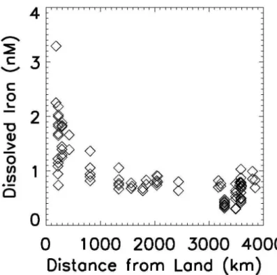
In Fig. 1, we plot the dissolved iron observations (>1000 m depth) from the

east-ern subtropical Pacific (latitudes 20–50◦N) as a function of approximate distance from

10

the continent. The obvious decline in iron concentrations as distance from the margin increases has been noted previously (Johnson et al., 1997, 2003). The data points within 200 km of the coastline were removed by our land-adjacent rule in the margin-excluded dataset. In addition, we removed all data from the locations in Fig. 1 that are ∼550–700 km offshore, retaining the other data points as more representative of

15

the open ocean. There may be influence of the continental margin even more than 1000 km offshore. We address the role of the continental source to the open ocean in our companion paper (MBb, this issue). Through a similar analysis, data was re-moved several locations near the Asian coast in the NW Pacific. We also exclude data from several papers that measured high iron concentrations attributed to sources

20

not included in the BEC model (riverine or hydrothermal – Mackey et al., 2002; Ker-guelen Islands runoff and sediments – Blain et al., 2001; Bucciarelli et al., 2001; and rapid advection from continental sources by the Antarctic Polar Front – L ¨oscher et al., 1997). These steps removed ∼48% of the observations, leaving 3176 observations in our open ocean subset (hereafter referred to as the “open ocean” data). This open

25

ocean subset is certainly more impacted by dust and less impacted by sedimentary iron sources than the data that has been excluded. However, in our companion paper we argue that even these open ocean iron concentrations are significantly influenced by the continental sedimentary source for iron (MBb, this issue).

(11)

BGD

4, 1241–1277, 2007

2.1 BEC model

The coupled biogeochemical elemental cycling (BEC) model (Moore et al., 2002a, 2004) includes ecosystem and biogeochemistry components including full carbonate chemistry dynamics. The model simulates four functional groups of phytoplankton (di-atoms, coccolithophores, diazotrophs, and picophytoplankton) and multiple potentially

5

growth limiting nutrients (nitrate, ammonium, phosphate, silicate, and dissolved iron). The BEC runs within the coarse resolution, POP ocean model that is part of the Com-munity Climate System Model (CCSM3.0) developed at the National Center for Atmo-spheric Research (Collins et al., 2006). The model includes 25 vertical levels with 8 levels in the upper 103 m, a longitudinal resolution of 3.6 degrees and a variable

lati-10

tudinal resolution, from 1–2 degrees, with the finer resolution near the equator (Collins et al., 2006; Yeager et al., 2006). All the nutrients/elements (C, O, N, P, Si, Fe) are simulated within the full ocean, 3D context with no restoring.

The BEC model reproduces basin-scale patterns of macronutrient distributions, cal-cification, biogenic silica production, nitrogen fixation, primary and export production

15

(Moore et al., 2002b, 2004). The model has recently been applied to quantify ocean biogeochemical sensitivity to variations in mineral dust deposition (iron inputs) (Moore et al., 2006), the feedbacks between denitrification and nitrogen fixation (Moore and Doney, 2007), and the ocean biogeochemical response to atmospheric deposition of inorganic nitrogen (Krishnamurthy et al., 2007). The results here are from the last year

20

of a 3000 year simulation. This is an extension of the 2000 year control simulation described by Moore and Doney (2007). Iron cycling in the BEC is discussed below, for further details on the BEC model please see Moore et al. (2002a, 2004) and Moore and Doney (2007).

2.2 Iron cycling in the BEC

25

Dissolved iron sources to the ocean in the BEC model include dissolution of iron from mineral dust particles deposited from the atmosphere and diffusion from shallower

(12)

BGD

4, 1241–1277, 2007

sediments, while a fraction of the scavenged iron is assumed lost to the sediments to balance these sources (Moore et al., 2004). There is one “dissolved” iron pool that is assumed to be bioavailable, with no distinction between soluble and colloidal forms. A constant fraction of the iron in mineral dust (here 2%) dissolves instanta-neously at the surface ocean, with some further iron release through a slower

dissolu-5

tion/disaggregation through the water column (Moore et al., 2004, MBb). Dust deposi-tion is from the climatology of Luo et al. (2003). The sedimentary Fe source is crudely incorporated as a constant flux of 2µmol/m2/day from sediments at the bottom of the ocean grid where depth is less than 1100 m (Moore et al., 2004). As noted by Moore et al. (2004) the coarse resolution ocean grid only weakly captures the bathymetry of the

10

continental shelves. Thus in many coastal/shelf regions the bottom level of the ocean grid is much deeper than the actual shelf regions, providing little iron to surface waters (see MBb, this issue).

Iron is removed from the dissolved pool through biological uptake by the phytoplank-ton and by particle scavenging. A fraction of the scavenged iron is added to the sinking

15

particulate pool and will remineralize deeper in the ocean, while the remainder is as-sumed lost to the sediments. Iron scavenging is parameterized in the BEC model based on the mass of scavenging particles and the ambient dissolved iron concentra-tion to crudely account for the presumed influences of iron binding ligands on scav-enging losses. Moore et al. (2004) described a scavscav-enging rate that consisted of a

20

base rate times the sinking particle flux divided by a reference particle flux. This ap-proach can be described more simply by combining the base rate and reference flux constant coefficients into one base scavenging rate (Febase) that is modified by the sinking particle flux (previously standing stock of POC was also included by Moore et al., 2004). The base scavenging rate (Febase = 0.01369 day−1) is thus a net

adsorp-25

tion rate to sinking particles, similar to the simplest Th scavenging models. The sinking POC flux and sinking particulate mineral dust fluxes were added to get the particle flux (ng/cm2/day) available to scavenge iron, and a maximum scavenging rate (MaxPE = 0.05476 day−1) was imposed (Eq. 1). Given the mean sinking fluxes in the model the

(13)

BGD

4, 1241–1277, 2007

base scavenging rates including the particle effect at 103 m depth, 502 m, and 2098 m would be 7.5e–4 day−1_{, 1.6e–4 day}−1_{,, and 8.1e-5 day}−1_{, respectively. These rates} would be further modified by the ambient iron concentrations. The sinking flux is dom-inated by POC in surface waters, but due to shorter remineralization length scales for POC, the sinking dust flux becomes important in the deep ocean. POC accounts for

5

93%, 67%, and 38% of the sinking mass flux at depths of 103 m, 502 m, and 2098 m, respectively.

ScavRate = Febase ∗ (sinking POC + sinking Dust), must be <= MaxPE (1) If dFe> HighFe then ScavRate=ScavRate + (dFe−HighFe) ∗ Chigh (2)

If dFe< LowFe then ScavRate=ScavRate ∗ (dFe/LowFe) (3)

10

ScavengedIron=dFe ∗ ScavRate (4)

The scavenging rate increases rapidly at higher iron concentrations (where dissolved iron (dFe) exceeds HighFe(0.6 nM), Chigh = 4286, Eq. 2) where iron is assumed to begin exceeding the concentrations of strong binding ligands, and progressively de-creased at low iron concentrations (LowFe = 0.5 nM, Eq. 3) to reflect protection from

15

scavenging losses due to strong iron binding ligands. The scavenging rate is multiplied by the ambient dissolved iron to get the amount removed by scavenging (Eq. 4), of which 10% (F Pfe) is put into the sinking particulate pool, with 90% of scavenged iron presumed lost to the sediments. Most ocean biogeochemical models assume that all scavenged iron is lost from the system (Archer and Johnson, 1999; Christian et al.,

20

2002; Aumont et al., 2003; Parekh et al., 2004, 2005). Gregg et al. (2003) add all scav-enged iron to the sinking pool to remineralize at depth, and Doney et al. (2006) send 60% to the sinking particulate pool. Moore et al. (2006) suggested some modifications to the original parameter values for the BEC (similar values are used here see Moore and Doney, 2007).

25

(14)

BGD

4, 1241–1277, 2007

3 Results

The observational dataset is heavily weighted towards the upper ocean with 66% of observations from depths less than 103 m, and 86% from depths less than 502 m. The dataset is also weighted strongly towards the Northern Hemisphere (75% of the data). The Southern Hemisphere data is mainly from the Southern Ocean (65% of S.H. data),

5

which we define as latitudes greater than 40.5◦S, with few observations in the lower lat-itudes, mainly in the South Atlantic (18%). There are also strong seasonal biases with only 3.3% of samples collected during winter months. Away from the high deposition regions, particularly at higher latitudes, winter often has maximum surface iron con-centrations due to deep mixing and weakened biological uptake. Spring months had

10

the most observations (46%) followed by summer (30%) and fall (21%). Spring is often a time of rapid biological drawdown of dissolved iron. Dust deposition typically has a strong seasonal component peaking during spring or summer months. Thus, iron can have a stronger seasonality, even at low latitudes, that typically seen in oceanographic data.

15

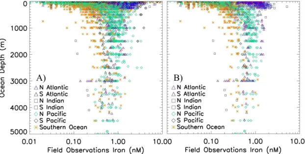
Vertical profiles of dissolved iron tend to follow two patterns: 1) a surface minimum due to surface depletion by biological uptake and scavenging processes; or 2) a surface maximum where there is strong influence by dust deposition events (Johnson et al., 1997a, 2003; de Baar and de Jong, 2001). All observations of dissolved iron are plotted against ocean depth in Fig. 2a, and a similar plot for the open ocean data in

20

Fig. 2b. The symbols used to indicate ocean basin of the samples in Fig. 2 are retained in later figures as well. There are some obvious, strong regional patterns in the iron distributions. The highest surface water concentrations are typically seen in the high dust deposition regions of the northern Indian Ocean and the low latitude North Atlantic (hereafter referred to as the “high deposition regions”), while the lowest surface values

25

are mainly in the Southern and Pacific oceans (Fig. 2). Low surface concentrations are (<0.1 nM) are also seen in some South Atlantic observations. The highest surface

(15)

BGD

4, 1241–1277, 2007

(Bruland et al., 2005) and in the Southern Ocean near the Kerguelen Islands (Blain et al., 2001; Bucciarelli et al., 2001). There is considerable variation in surface iron concentrations within basins reflecting differential inputs and removal rates.

In the open ocean dataset, the mean surface iron concentration (_{<=20 m) for all} areas except the high deposition regions is 0.25±0.23 nM (where 0.23 is the standard

5

deviation), and the mean in the high deposition regions is 0.76±0.27 nM. The area outside the high deposition regions can be further subdivided between HNLC zones (where annual surface nitrate concentrations exceed 1.0µM in the World Ocean Atlas

2001, Conkright et al., 2001) and the non-HNLC regions. The mean concentration for the HNLC regions is 0.15±0.16 nM and for the non-HNLC regions the mean is

10

0.27±0.24 nM. It is notable that the iron-limited HNLC regions have mean dissolved iron surface concentrations only moderately lower than the non-HNLC areas. These means are considerably higher than the mean surface value of 0.07 nM calculated by Johnson et al. (1997a). This reflects additional sampling of surface waters shortly after dust deposition events, which in the North Pacific for example can raise surface

15

water concentrations from background levels of<0.2 nM to values in excess of 0.6 nM

(Bruland et al., 1994; Wu et al., 2001; Johnson et al., 2003), increased high latitude sampling early and late in the growing season when deeper mixing may increase iron concentrations, and possibly systematic differences between groups measuring iron.

Many of the elevated deep water concentrations are associated with continental

mar-20

gins and do not appear in our open ocean subset (compare Figs. 2a and b) most no-tably in the Pacific data. Deep water values in the open ocean dataset range mainly between ∼0.2–1.0 nM, with the Southern Ocean showing consistently low values and the North Atlantic and North Pacific having higher, similar concentrations. Unlike the North Atlantic data which typically have a surface maximum and decline with depth,

25

the Arabian Sea data tend to increase modestly with depth in the upper ocean (Fig. 3). This may be partially due to lower scavenging losses in the sub-oxic waters below the euphotic zone (Measures and Vink, 1999).

There is a clear signal from dust deposition in the depth-resolved iron data with the 1254

(16)

BGD

4, 1241–1277, 2007

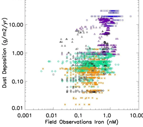
highest concentrations in the open ocean dataset all in the high deposition regions, and with the lowest upper ocean iron concentrations in the low deposition areas of the Southern Ocean and the equatorial Pacific. In Fig. 3, we plot all dissolved iron obser-vations from the open ocean dataset against the climatological annual dust deposition estimated by Luo et al. (2003) for the late 20th century. There is considerable

uncer-5

tainty in these model estimates of dust deposition, but some general patterns seem fairly robust. Dust deposition varies over three orders of magnitude while most of the iron observations fall within a much narrower range (∼two orders of magnitude). This reflects the non-linear nature of iron removal processes, although variations in aerosol iron solubility may also play a role, as the lower deposition areas generally farther from

10

source regions may have higher solubilities (see Mahowald et al., 2005, and references therein). The regions beneath the major dust plumes in the North Atlantic and northern Indian oceans receive two orders of magnitude higher dust deposition than most other areas. The North Pacific receives ∼2–5 times more dust than most Southern Ocean sites, although some of the very lowest deposition rates are in the equatorial Pacific.

15

There is some overlap across all the regions, some North Atlantic sites receive low dust levels, and the South Atlantic sites span the range from low to high deposition. A few Southern Ocean regions receive more than 1 g dust/m2/yr (Fig. 3). For each dust deposition rate there is typically a wide range of observed iron concentrations. This likely reflects errors in the dust deposition, variable removal by biological uptake

20

and particle scavenging, influence by other Fe sources, and variations in depth of the sample (although the database is strongly weighted towards the upper ocean).

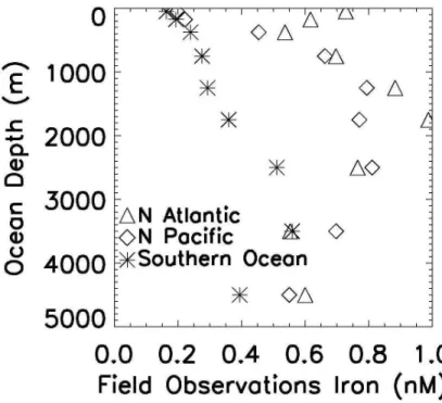
There was sufficient data in the North Atlantic, North Pacific, and Southern Ocean to calculate mean profiles of dissolved iron from the open ocean dataset (Fig. 4). In the upper ocean mean dissolved iron concentrations were quite low in the Southern

25

Ocean (0.16 nM upper 100 m) and in the North Pacific (0.20 nM upper 100 m), with much higher iron levels in the North Atlantic (0.73 nM). There was a sub-surface min-imum in the North Atlantic between 100–250 m depth, noted previously (Wu et al., 2001; Wu and Boyle, 2001; Sedwick et al., 2005; Bergquist and Boyle, 2006). Below

(17)

BGD

4, 1241–1277, 2007

250 m the profiles for the North Atlantic and North Pacific basins are similar, despite a roughly two orders of magnitude difference in dust deposition (Figs. 3 and 4). This sim-ilarity was noted previously in a much smaller dataset by Johnson et al. (1997a). The Southern Ocean has much lower mean concentrations below 250 m with the largest difference between 1000–1500 m by a factor of ∼2.6–2.9. Values appear to converge

5

somewhat in the deepest ocean, but there were few observations below 2000 m (see Fig. 2b). We calculated mean iron concentrations below 500 m depth for these basins as 0.37±0.19 (n=96) for the Southern Ocean, 0.74±0.33 nM (n=107) for the North Atlantic, and 0.74±0.21 nM (n=232) for the North Pacific. The North Pacific data may reflect a strong influence from continental sources (see Fig. 1 and MBb). If all

10

observations are included (rather than just the open ocean subset) mean concentra-tions are higher in the North Pacific (0.87±0.37 nM, n=468) than in the North Atlantic (0.76±0.31 nM, n=149), reflecting in part more sampling near the continents in the North Pacific. The Southern Ocean mean for all data was 0.46±0.28 nM (n=160).

The BEC simulated iron distributions are compared with the open ocean

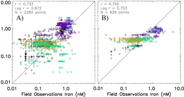
observa-15

tions in Fig. 5 (with model values extracted from the same month, depth, and location as the observations). There is a broad agreement between the model and the obser-vations in surface waters (r-correlation coefficient of 0.73, Fig. 5a). However, the model tends to overestimate iron concentrations, particularly at the lower iron concentrations, below ∼0.3 nM. Values at the high end of iron concentrations also tend to be

some-20

what too high in the model. There are a couple of dozen points in the Atlantic basin where the model drastically overestimates iron concentrations (Fig. 5a). This reflects the coarse resolution of the ocean model and the atmospheric model used to generate the dust deposition field. Due to the sharp gradients involved small shifts in the location of the dust plume can create large errors in the model-data comparison, leading to the

25

model estimating high iron concentrations at a number of points where low iron was observed. In subsurface waters the model again is relatively well correlated with the observations (r=0.76, 0.70 for log-transformed data, Fig. 5b). In contrast to surface waters the model underestimates concentrations at the high end (>0.6 nM) and again

(18)

BGD

4, 1241–1277, 2007

tends to overestimate iron concentrations at the low end (< ∼0.3–4 nM) (Fig. 5b). There

is significant seasonal variability in the surface and subsurface iron concentrations in the high deposition regions (not shown).

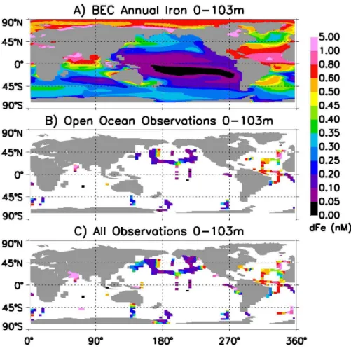
We compare spatial plots of annual mean BEC simulated iron with the observations, illustrating the open ocean subset and full dataset observations (Figs. 6–8). Looking

5

at the surface water observational data (0–103 m) dissolved iron concentrations are typically quite low (<0.2 nM) outside the high deposition regions (Fig. 6). The model

displays qualitatively similar patterns, but often overestimates the absolute concentra-tions in the low iron regions. In part this is due to seasonal entrainment of iron at higher latitudes (and observational under-sampling during winter months), but the model

esti-10

mates were too high even when comparing with monthly model output from the same months as the observations (Fig. 5).

In subsurface waters the tendency for the model to overestimate iron concentrations away from the high deposition regions in even more apparent (Fig. 7). Given our inputs of dissolved iron from dust deposition, it is apparent that strong scavenging removal of

15

iron in the upper water column below the euphotic zone is necessary to reproduce the observed concentrations. The model tends to underestimate the subsurface dissolved iron concentrations in the high deposition regions (Fig. 7). In the deep ocean (>500 m)

the simulated iron concentrations are lowest in the eastern Equatorial Pacific followed by the Southern Ocean, with high concentrations (>0.6 nM) in the high deposition re-20

gions (Fig. 8a). The model output in the deep North Pacific has concentrations in be-tween the North Atlantic and Southern Ocean regions, a pattern suggested by Parekh et al. (2005) for the real ocean. However, the observations don’t strongly display this pattern, but have values in the North Pacific that are similar to the high deposition regions, except for the data closest to the central portion of the gyre where iron

con-25

centrations are lower. Examining the full dataset in this region it appears that coastal iron sources extend influence well into the North Pacific gyre, partially compensating for the lower dust inputs from the atmosphere (Figs. 1 and 8c, see also MBb). The sim-ulated iron concentrations in the deep Southern Ocean are considerably higher than

(19)

BGD

4, 1241–1277, 2007

observations. The model only weakly captures the strong contrast between deeper iron concentrations in the North Pacific and Southern Ocean (Figs. 7 and 8).

In the surface observations from the Ross Sea and off the western coast of North and South America, high concentrations are apparent in the observations near land, declining quickly offshore (Fig. 6c). A similar pattern can be seen in the subsurface

5

observations in the Ross Sea, the eastern North Atlantic, the eastern North Pacific, the gulf of Alaska extending southwards from land, and in the western North Pacific (Fig. 7c). At these subsurface depths (103–502 m) the coastal source can often be seen to extend farther offshore, than in surface waters (Figs. 6c and 7c). This pattern extends into the deep ocean as well (Fig. 1 and Fig. 8c, see also MBb) due to reduced

10

particle flux and scavenging losses at depth.

4 Discussion

We have seen strong regional to basin scale trends in the observed distributions of dissolved iron in the world ocean. These patterns confirm the strong role of atmo-spheric dust deposition as a source of dissolved iron to the open ocean (Figs. 2 and

15

3). However, this dust-iron relationship is highly nonlinear (Fig. 3), reflecting the strong biological influence on iron distributions. Mean deep ocean iron concentrations are similar in the North Pacific and North Atlantic, despite the much higher dust inputs to the Atlantic (Fig. 4). It appears that the coastal iron source may contribute substan-tially to the open ocean in the North Pacific, parsubstan-tially compensating for the lower dust

20

inputs. We address the relative roles of atmospheric and sedimentary iron sources in the companion paper (MBb, this issue).

Despite a wide range of dust inputs from the atmosphere, the surface iron distribu-tions exhibit a strong bi-modal distribution, with peaks at ∼0.1–0.2 nM and at ∼0.6– 0.8 nM. These patterns likely result from interactions with the organic ligands that bind

25

nearly all the dissolved iron in seawater. These interactions appear to set up dis-tinct scavenging regimes for dissolved iron in the oceans, depending on the balance

(20)

BGD

4, 1241–1277, 2007

between iron sources and sinks. At very high iron inputs, as in the high deposition regions, the strong binding ligands can become saturated, and scavenging rates will increase as an increasing proportion of iron is bound to weaker ligands or exists as free inorganic iron. Some removal of the colloidal size class of ligands will occur due to aggregation and settling processes, but this will rapidly be replenished in surface

5

waters, where biological processes releasing the ligands are active, and perhaps in the deeper ocean during remineralization of sinking organic matter. At lower iron input levels, this aggregation and removal of the colloidal size class will decrease surface dissolved iron concentrations to lower concentrations. Biological uptake will also re-move substantial amounts of dissolved iron, particularly as some larger phytoplankton

10

engage in luxury uptake of iron. At very low iron input levels, or as these processes deplete iron down to very low levels (<0.1–0.15 nM), the loss rate for dissolved iron

will likely decline. A higher proportion of the ligand-bound iron may exist in the soluble size class (Nishioka et al., 2001, 2005) and, therefore, will not be subject to signifi-cant aggregation/scavenging removal. Also, the phytoplankton uptake will decrease as

15

available iron approaches the half-saturation values for iron uptake and phytoplankton become increasingly iron stressed (growing more slowly and decreasing their cellular Fe/C ratios). Thus, outside the high iron input areas, dissolved iron concentrations will tend to be depleted to low levels in surface waters (<0.2 nM), over a fairly wide range

of iron inputs from mineral dust and other sources.

20

Our assumption in the BEC model that scavenging rates progressively decrease as iron decreases below 0.5 nM is incorrect and leads to an overestimation of dissolved iron concentrations at the low end of observations (Figs. 5–9). In the companion pa-per, we demonstrate a much better BEC fit to observations using a first-order, particle-dependent scavenging rate, with no dependence on ambient iron concentration for

25

iron values below 0.6 nM (MBb, this issue). Our model results also suggest that there must be significant removal of dissolved iron in subsurface waters, where the iron con-centrations are typically well below 0.6 nM, for the model to match the observed iron distributions (MBb, this issue). Thus, aggregation and scavenging removal of the

(21)

col-BGD

4, 1241–1277, 2007

loidal iron pool likely plays a key role in determining dissolved iron concentrations (Wu et al., 2001; de Baar and de Jong, 2001; Nishioka et al., 2001).

At present there are only a few studies of the size-fractionation of “dissolved” iron between the soluble and colloidal pools. The soluble pools have been noted to have strongly nutrient type profiles, while the colloidal fraction is more variable, often with a

5

subsurface/upper thermocline minimum (Wu et al., 2001). Soluble Fe concentrations in surface waters have been measured at ∼0.1 nM in oligotrophic (presumably N or P limited) regions (Wu et al., 2001; Wen et al., 2006), although Cullen et al. (2006) found values ranging between 0.04–0.28 nM in the Atlantic. Somewhat lower values of ∼0.05 nM have been reported in the iron-limited subarctic NE Pacific and Southern

10

Ocean (Nishioka et al., 2001; 2005). In these studies, the concentration of soluble iron increased steadily with depth, to values ∼0.2–0.4 nM below several hundred meters.

The increasing soluble iron concentrations with depth may partially explain the ob-served trend towards increasing iron concentrations with increasing depth (Figs. 6–8, see also Fig. 4 in MBb). Other factors also likely contribute, including strong biological

15

drawdown in surface waters, and weaker scavenging in the deep ocean due to lower particle concentrations. Aggregation and scavenging of the colloidal iron fraction may also explain the observed subsurface minimum concentration for colloidal iron (Wu et al., 2001). In these relatively shallow, subsurface waters, iron inputs and likely the pro-duction of the organic ligands are lower than in surface waters, but particle flux, colloidal

20

aggregation, and scavenging rates are likely fairly high. Thus, even in high deposition regions, much of the colloidal fraction may be removed by aggregation and scaveng-ing. The release of this scavenged iron, along with lower particle flux and scavenging rates, then leads to higher iron concentrations in the deep ocean. Scavenging rates would still increase as dissolved iron rose above ∼0.6–0.7 nM, setting an upper limit

25

on the deep ocean concentrations (Fig. 8c), as suggested by Johnson et al. (1997a). At any one location, the observed profiles are likely fairly dynamic and dependent on the balance between the various local sources and sinks and advective processes (Wu and Luther, 1997; Wu and Boyle, 2002). Nishioka et al. (2001) noted strong temporal

(22)

BGD

4, 1241–1277, 2007

variations in the soluble iron fraction at depth. There is likely a dynamic, rapid turnover and exchange of iron amongst the various pools, both at the surface and in the deeper ocean (de Baar and de Jong, 2001; Bruland and Lohan, 2004; Cullen et al., 2006).

A global collection of dissolved iron observations has now accumulated that is suf-ficient to place some strong constraints on ocean biogeochemical models. There

ap-5

pears to be substantial scavenging removal of iron in areas where ambient concen-trations are well below 0.6 nM. Thus, models that assume scavenging removal only when iron concentrations exceed this threshold will tend to overestimate subsurface iron concentrations and subsurface Fe inputs to the euphotic zone. This will tend to over-emphasize the subsurface iron source and underestimate the importance of dust

10

deposition as a driver of ocean biogeochemical cycling. Thus, it is critical that mod-els be evaluated against observations both for surface fields, and for the subsurface depths that drive much of the iron input to surface waters (see also MBb).

In the high deposition regions, observed iron concentrations are often well above 0.6 nM, although this signal appears to be removed by scavenging over relatively short

15

timescales (weeks to months), allowing for limited advection. The mean surface iron concentration for areas outside the high deposition regions is 0.25±0.23 nM, and the mean in the high deposition regions is 0.76±0.27 nM. This is only a three-fold differ-ence in mean iron concentrations, despite variations in iron inputs of several orders of magnitude. The mean concentration for the HNLC regions is 0.15±0.16 nM, only

mod-20

estly lower than for the non-HNLC regions (excluding high deposition areas) where the mean is 0.27±0.24 nM. These averages include sporadic increases due to dust depo-sition events (i.e., Bruland et al., 1994; Johnson et al., 2003), otherwise surface values are typically below 0.2 nM. The deep North Pacific has similar deep ocean concen-trations to the high deposition regions, with strong lateral gradients – high iron values

25

near the continental margins, decreasing towards the center of the basin. Another key metric is how well models can reproduce the binned distributions of iron observations (MBb, this issue).

(23)

BGD

4, 1241–1277, 2007

database over several decades, but there is still much we do not know about the marine iron cycle. The observational database for iron is still a tiny fraction of that available for other key nutrients. The size-fractionation of the dissolved pool and the relative roles of soluble and colloidal classes are only just beginning to be addressed. Numerous questions remain concerning the particle scavenging, bioavailability, photochemistry,

5

and turnover times of the various iron pools The iron fertilization experiments have demonstrated the key role iron plays in governing ocean productivity and biogeochem-ical cycling (de Baar et al., 2005). Fully unraveling all the mechanisms and processes controlling iron cycling in the modern ocean, and incorporating these results into ocean biogeochemical models to understand the role of iron cycling in future and past climate

10

regimes, will be a key area of research in the coming decades.

Acknowledgements. We would like to thank all the researchers, technicians, and students

who made the iron measurements and for making the data publicly available. Also thanks to P. Parekh, M. Follows, and E. Boyle for publishing their iron observations compilation. This work is funded by a National Science Foundation grant (NSF OCE-0452972 to J. K. Moore)

15

and the UCI Research Experience for Undergraduates (REU) program funded by the National Science Foundation (NSF ATM-0453295 to J. K. Moore).

References

Archer, D. E. and Johnson, K.: A model of the iron cycle in the ocean, Global Biogeochem. Cycles, 14, 269–279, 2000.

20

Aumont, O., Maier-Reimer, E., Blain, S., and Monfray, P.: An ecosystem model of the global ocean including Fe, Si, P co-limitations, Global Biogeochem. Cycles, 17, 1060, doi:10.1029/2001GB001745, 2003.

Bacon, M. P. and Anderson, R. F.: Distribution of Thorium isotopes between dissolved and particulate forms in the deep sea, J. Geophys. Res., 87, 2045–2056, 1982.

25

Balistrieri, L., Brewer, P. G., and Murray, J. W.: Scavenging residence times of trace metals and surface chemistry of sinking particles in the deep ocean, Deep-Sea Res., 28, 101–121, 1981.

(24)

BGD

4, 1241–1277, 2007

Bergquist, B. A. and Boyle, E. A.: Dissolved iron in the tropical and subtropical Atlantic Ocean, Global Biogeochem. Cycles, 20, GB1015, doi:10.1029/2005GB002505, 2006.

Berman-Frank, I., Cullen, J. T., Shaked, Y., Sherrell, R. M., and Falkowski, P. G.: Iron availability, cellular iron quotas, and N fixation in Trichodesmium, Limnol. Oceanogr., 46, 1249–1260, 2001.

5

Blain, S., Treguer, P., Belviso, S., Bucciarelli, E., Denis, M., Desbre, S., Fiala, M., Jezequel, V. M., LeFevre, J., Mayzaud, P., Marty, J., and Razouls, S.: A biogeochemical study of the island mass effect in the context of the iron hypothesis: Kerguelen Islands, Southern Ocean, Deep-Sea Res. I, 48, 163–187, 2001.

Bowie, A. R., Achterberg, E. P., Blain, S., Boye, M., Croot, P. L., de Baar, H. J. W., Laan, P.,

10

Sarthou, G., and Worsfold, P. J.: Shipboard analytical intercomparison of dissolved iron in surface waters along a north-south transect of the Atlantic Ocean, Mar. Chem., 84, 19–34, 2003.

Bowie, A. R., Achterberg, E. P., Croot, P. L., de Baar, H. J. W., Laan, P., Moffett, J. W., Ussher, S., and Worsfold, P. J.: A community-wide intercomparison exercise for the determination of

15

dissolved iron in seawater, Mar. Chem., 98, 81–99, 2006.

Boyd, P. W. and Doney, S. C.: Modelling regional responses by marine pelagic ecosystems to global climate change, Geophys. Res. Lett., 29(16), 53–1 to 53–4, doi:10.1029/2001GL014130, 2002.

Boyd, P. W., Watson, A. J., Law, C. S., Abraham, E. R., Trull, T., Murdoch, R., Bakker, C. E.,

20

Bowei, A. R., Buesseler, K. O., Chang, H., Charette, M., Croot, P., Downing, K., Frew, R., Gall, M., Hadfield, M., Hall, J., Harvey, M., Jameson, G., LaRoche, J., Liddicoat, M., Ling, R., Maldonado, M.T., McKay, R.M., Nodder, S., Pickmere, S., Pridmore, Rintoul, S., Safi, K., Sutton, P., Strzepek, R., Tanneberger, K., Turner, S., Waite, A., and Zeldis, J.: A mesoscale phytoplankton bloom in the polar Southern Ocean stimulated by iron fertilization, Nature,

25

407, 695–702, 2000.

Bolye, E. A.: What controls dissolved iron concentrations in the world ocean – A comment, Mar. Chem., 57, 163–167, 1997.

Bruland, K. W., Orians, K. J., and Cowen, J. P.: Reactive trace metals in the stratified central North Pacific, Geochimica et Cosmocimica Acta, 58, 3171–3182, 1994.

30

Bruland, K. W. and Lohan, M. C.: The control of trace metals in seawater. Chapter 2 in The Oceans and Marine Geochemistry, Vol. 6 (Ed. Harry Elderfield) in Treatise on Geochemistry, edited by: Holland, H. D. and Turekian, K. K., 2004.

(25)

BGD

4, 1241–1277, 2007

Bruland, K. W., Rue, E. L., Smith, G. J., and DiTullio, G. R.: Iron, macronutrients and diatom blooms in the Peru upwelling regime : brown and blue waters of Peru, Mar. Chem., 93, 81–103, 2005.

Bucciarelli, E., Blain, S., and Treguer, P.: Iron and manganese in the wake of the Kerguelen Islands (Southern Ocean), Mar. Chem. 73, 21–36, 2001.

5

Burd, A. B., Jackson, G. A., and Moran, S. B.: A coupled adsorption-aggregation model for the POC/234Th ratio of marine particles. Deep-Sea Res. I., 47, 103–120, 2000.

Chase, Z., Johnson, K.S., Elrod, V.A., Plant, J.N., Fitzwater, S.E., Pickell, L., Sakamoto, C.M. : Manganese and iron distributions off central California influenced by upwelling and shelf width. Mar. Chem., 95, 235-254, 2005.

10

Christian, J. R., Verschell, M. A., Murtugudde, R., Busalacchi, A. J., and McClain, C. R.: Bio-geochemical modeling of the tropical Pacific Ocean II. Iron biogeochemistry, Deep-Sea Res. II, 49, 545–565, 2002.

Clegg, S. L. and Sarmiento, J. L. : The hydrolytic scavenging of metal ions by marine particulate matter, Prog. Oceanogr., 23, 1–21, 1989.

15

Coale, K. H., Gordon, R. M., and Wang, X. : The distribution and behavior of dissolved and particulate iron and zinc in the Ross Sea and Antarctic circumpolar current along 170oW, Deep-Sea Res. I, 52, 295–318, 2005.

Coale, K. H., Johnson, K. S., Fitzwater, S. E., Gordon, R. M., Tanner, S., Chavez, F. P., Ferioli, L., Sakamoto, C., Rogers, P., Millero, F., Steinberg, P., Nightingale, P., Cooper, D., Cochlan,

20

W. P., Landry, M. R., Constantiou, J., Rollwagen, G., Trasvina, A., and Kudela, R.: A mas-sive phytoplankton bloom induced by an ecosystem-scale iron fertilization experiment in the equatorial Pacific Ocean, Nature, 383, 495–501, 1996.

Coale, K. H., Johnson, K. S., Chavez, F. P., Buesseler, K. O., Barber, R. T., et al.: Southern Ocean Iron Enrichment Experiment: Carbon cycling in high- and low-Si waters, Science,

25

304, 408–414, 2004.

Collins W. D., Blackmon, M., Bitz, C. M., Bonan, G. B., Bretherton, C. S., Carton, J. A., Chang, P., Doney, S., Hack, J. J., Kiehl, J. T., Henderson, T., Large, W. G., McKenna, D., and Santer, B. D.: The Community Climate System Model: CCSM3, J. Climate, 19, 2122–2143, 2006. Conkright, M. E., Locarnini, R. A., Garcia, H. E., O’Brien, T. D., Boyer, T. P., Stevens, C., and

30

Antonov, J. I.: World Ocean Atlas 2001: Objective analysis, data statistics, and figures, CD ROM documentation. National Oceanographic Data Center, Silver Spring, MD, 2002. Cullen, J. T., Bergquist, B. A., and Moffett, J. W. : Thermodynamic characterization of the

(26)

BGD

4, 1241–1277, 2007

partitioning of iron between soluble and colloidal species in the Atlantic Ocean, Mar. Chem., 98, 295–303, 2006.

de Barr, J. W. H., Boyd, P. W., Coale, K. H., Landry, M. R., Tsuda, A., Assmy, P., Bakker, D. C. E., Boze, Y., Barber, R. T., Brzezinski, M. A., Buesseler, K. O., Boy ´e, M., Croot, P. L., Gervais, F., Gorbunov, M. Y., Harrison, P. J., Hiscock, W. T., Laan, P., Lancelot, C., Law, C.

5

S., Levasseur, M., Marchetti, A., Millero, F. J., Nishioka, J., Nojiri, Y., van Oijen, T., Riebesell, U., Rijkenberg, M.J.A., Saito, H., Takeda, S., Timmermans, K. R., Veldhuis, M. J. W., Waite, A. M., and Wong, C. S.: Synthesis of iron fertilization experiments: From the Iron age in the Age of Enlightenment, J. Geophys. Res., 110, C09S16, doi:10.1029/2004CJ002601, 2005. de Baar, H. J. W. and De Jong, J. T. M.: Distributions, sources and sinks of iron in seawater, in:

10

Biogeochemistry of Iron in Seawater, edited by: Turner, D. and Hunter, K. A., IUPAC Book Series on Analytical and Physical Chemistry of Environmental Systems, 7, 123–253, 2001. de Baar, H. J. W., de Jong, J. T. M., Nolting, R. F., Timmermans, K. R., van Leeuwe, M. A.,

Bathmann, U., Rutgers van der Loeff, M., and Sildam, J.: Low dissolved Fe and the absence of diatom blooms in remote Pacific waters of the Southern Ocean, Mar. Chem., 66, 1–34,

15

1999.

Dutkiewicz, S., Follows, M., and Parekh, P.: Interactions of the iron and phosphorus cycles: A three-dimensional model study, Global Biogeochem. Cycles, 19, GB1021, doi:10.1029/2004GB002342, 2005.

Falkowski, P. G.: Evolution of the nitrogen cycle and its influence on the biological sequestration

20

of CO2 in the ocean, Nature, 387, 272–275, 1997.

Gregg, W., Ginoux, P., Schopf, P. S., and Casey, N. W.: Phytoplankton and iron: validation of a global three-dimensional ocean biogeochemical model, Deep-Sea Res. II, 50, 3143–3169, 2003.

Gruber, N.: The dynamics of the marine nitrogen cycle and its influence on atmospheric CO₂

25

variations, In: The Ocean Carbon Cycle, Eds. Follows, M., Oguz, T., Kluwer Academic Pub-lishers, Netherlands, 97–148, 2004.

Honeyman, B. D., Balistrieri, L. S., and Murray, J. W.: Oceanic trace metal scavenging: the importance of particle concentration, Deep-Sea Res., 35, 227–246, 1988.

Honeyman, B. D. and Santschi, P. H.: A Brownian-pumping model for oceanic trace-metal

30

scavenging: evidence from Th isotopes, J. Mar. Res., 47, 951–992, 1989.

Johnson, K, Gordon, M. R, and Coale, K. H.: What controls dissolved iron concentrations in the world ocean?, Mar. Chem., 57, 137–161, 1997a.

(27)

BGD

4, 1241–1277, 2007

Johnson, K., Gordon, M. R, and Coale, K. H.: What controls dissolved iron concentrations in the world ocean? – Authors closing comments, Mar. Chem., 57, 181–186, 1997b.

Johnson, K. S., Chavez, F. P., and Friederich, G. E. Continental-shelf sediment as a primary source of iron for coastal phytoplankton. Nature, 398, 697–700, 1999.

Johnson, K.S ., Elrod, V. A., Fitzwater, S. E., Plant, J. N., Chavez, F. P., Tanner, S. J., Gordon,

5

R. M., Westphal, D. L., Perry, K. D., Wu, J., and Karl, D. M.: Surface ocean-lower atmo-sphere interactions in the Northeast Pacific Ocean Gyre: Aerosols, iron, and the ecosystem response. Global Biogeochem. Cycles, 17, 1063, doi:10.1029/2002GB002004, 2003. Krishnamurthy, A., Moore, J. K., Zender, C. S., and Luo, C.: The Effects of Atmospheric

In-organic Nitrogen Deposition on Ocean Biogeochemistry, J. Geophys. Res.-Biogeosci., in

10

press, 2007.

Lef `evre, N. and Watson, A. J.: Modeling the geochemical cycle of iron in the oceans and its impact on atmospheric CO2 concentrations, Global Biogeochem. Cycles, 13, 727–736, 1999.

L ¨oscher, B. M., de Baar, H. J. W., de Jong, J. T. M.,and Goeyens, L.: The distribution of Fe in

15

the Antarctic Circumpolar Current, Deep Sea-Res. II., 143–187, 1997.

Luo, C., Mahowald, N., and del Corral, J., Sensitivity study of meteorological parameters on mineral aerosol mobilization, transport and distribution, J. Geophys. Res., 108(D15), 4447, doi:10.1029/2003JD0003483, 2003.

Luther III, G. W. and Wu, J.: What controls dissolved iron concentrations in the world ocean? –

20

a comment. Mar. Chem., 57, 173–179, 1997.

Mackey, D. J., O’Sullivan, J. E., and Watson, R. J.: Iron in the western Pacific: a riverine or hydrothermal source for iron in the Equatorial Undercurrent?, Deep-Sea Res. I, 49, 877– 893, 2002.

Mahowald, N. M., Baker, A. R., Bergametti, G., Brooks, N., Duce, A., Jickells, T. D., Kubliay, N.,

25

Prospero, J. M., and Tegen, I.: Atmospheric global dust cycle and iron inputs to the ocean, Global Biogeochem. Cycles, 19, GB4025, doi:10.1029/2004GB002402, 2005.

Martin, J.H .: Iron as a limiting factor in oceanic productivity, in: Falkowski, P. G. and Woodhead, A. D., Primary Productivity and Biogeochemical Cycles in the Sea. Plenum Press, New York, 123–137, 1992.

30

Martin, J. H., Gordon, R. M., and Fitzwater, S. E.: The case for iron, Limnol. Oceanogr., 36, 1793–1802, 1991.

Measures, C. I. and Vink, S.: Seasonal variations in the distribution of Fe and Al in the surface

(28)

BGD

4, 1241–1277, 2007

waters of the Arabian Sea. Deep-Sea Research II, 46, 1597–1622, 1999.

Measures, C. I. and Vink, S.: Dissolved Fe in the upper waters of the Pacific sector of the Southern Ocean, Deep-Sea Res. II, 48, 3913–3941, 2001.

Michaels, A. F., Karl, D. M., and Capone, D. G.: Elemental stoichiometry, new production, and N fixation, Oceanography, 14(4), 68–77, 2001.

5

Moore, J. K., Doney, S. C., Kleypas, J. C., Glover, D. M., and Fung, I. Y.: An intermediate complexity marine ecosystem model for the global domain, Deep-Sea Res. II, 49, 403–462, 2002a.

Moore, J. K., Doney, S. C., Glover, D. M., and Fung, I. Y.: Iron cycling and nutrient limitation patterns in surface waters of the world ocean, Deep-Sea Res. II, 49, 463–508, 2002b.

10

Moore, J. K., Doney, S. C., and Lindsay, K.: Upper ocean ecosystem dynamics and iron cycling in a global three-dimensional model, Global Biogeochem. Cycles, 18, GB4028, doi:10.1029/2004GB002220, 2004.

Moore, J. K., Doney, S. C., Lindsay, K., Mahowald, N., and Michaels, A. F.: N fixation am-plifies the ocean biogeochemical response to decadal timescale variations in mineral dust

15

deposition, Tellus B, 58B, 560–572, 2006.

Moore, J. K. and Doney, S. C.: Iron availability limits the ocean nitrogen inventory stabilizing feedbacks between marine denitrification and nitrogen fixation, Global Biogeochem. Cycles, GB2001, doi:10.1029/2006GB002762, 2007.

Moore J. K. and Braucher, O.: Sedimentary and mineral dust sources of dissolved iron to the

20

world ocean, Biogeosci. Discuss., 4, 1279–1327, 2007.

Nishioka, J., Takeda, S., Wong, C. S., and Johnson, W. K.: Size-fractionated iron concentrations in the northeast Pacific Ocean: distribution of soluble and colloidal iron, Mar. Chem., 74, 157–179, 2001.

Nishioka, J., Takeda, S., de Baar, H. J. W., Croot, P. L., Boye, M., Laan, P., and Timmermans, K.

25

R.: Changes in the concentration of iron in different size fractions during an iron fertilization experiment in the open Southern Ocean, Mar. Chem., 95, 51–63, 2005.

Parekh, P, Follows, M. J, and Boyle, E. A.: Decoupling of iron and phosphate in the global ocean, Global Biogeochem. Cycles, 19, GB2020, doi:10.1029/2004GB002280, 2005. Parekh, P., Follows, M. J., Dutkiewicz, S., and Ito, T.: Physical and biological regulation of

30

the soft tissue carbon pump. Paleoceanography, 21, PA3001, doi:10.1029/2005PA001258, 2006.