HAL Id: hal-00317050
https://hal.archives-ouvertes.fr/hal-00317050
Submitted on 1 Jan 2003
HAL is a multi-disciplinary open access
archive for the deposit and dissemination of
sci-entific research documents, whether they are
pub-lished or not. The documents may come from
teaching and research institutions in France or
abroad, or from public or private research centers.
L’archive ouverte pluridisciplinaire HAL, est
destinée au dépôt et à la diffusion de documents
scientifiques de niveau recherche, publiés ou non,
émanant des établissements d’enseignement et de
recherche français ou étrangers, des laboratoires
publics ou privés.
Comparison of travelling ionospheric disturbance
measurements with thermosphere/ionosphere model
results
Ya. F. Ashkaliev, G. I. Gordienko, Ch. Jacobi, Yu. G. Litvinov, V. V.
Vodyannikov, A. F. Yakovets
To cite this version:
Ya. F. Ashkaliev, G. I. Gordienko, Ch. Jacobi, Yu. G. Litvinov, V. V. Vodyannikov, et al..
Compari-son of travelling ionospheric disturbance measurements with thermosphere/ionosphere model results.
Annales Geophysicae, European Geosciences Union, 2003, 21 (4), pp.1031-1037. �hal-00317050�
Annales Geophysicae (2003) 21: 1031–1037 c European Geosciences Union 2003
Annales
Geophysicae
Comparison of travelling ionospheric disturbance measurements
with thermosphere/ionosphere model results
Ya. F. Ashkaliev1, G. I. Gordienko1, Ch. Jacobi2, Yu. G. Litvinov1, V. V. Vodyannikov1, and A. F. Yakovets1
1Institute of Ionosphere, Almaty, 480020, Kazakhstan
2University of Leipzig, Institute for Meteorology, Stephanstr. 3, 04103 Leipzig, Germany
Received: 14 June 2002 – Revised: 5 September 2002 – Accepted: 18 September 2002
Abstract. Comparisons of modeled and measured responses
of the ionosphere to the passage of atmospheric gravity waves are made for data recorded by an ionosonde located at Almaty (76◦550E, 43◦150N) from June 2000 until May 2001. Temporal variations of the altitude (hmF) and electron content (NmF) of the F-layer peak are used for comparisons. A significant part of the observations showed well-defined wave structures on the hmF, NmF and other parameter vari-ations observed throughout the entire nights. Both the mod-eling study and measurements showed that, as the F-layer is lifted by the positive surge in gravity wave, the electron con-tent at the F-layer peak decreases, with the slab thickness be-ing increased as well. Subsequently, the opposite happens as hmF falls below its equilibrium value. Some discrepancy be-tween the model and experimental results related to the phase difference between hmF and NmF variations is revealed.
Key words. Ionosphere (ionosphere-atmosphere
interac-tion, ionospheric disturbances)
1 Introduction
Internal atmospheric gravity waves (AGWs) play an impor-tant role in the dynamics of the middle and upper atmo-sphere. Propagating through the thermosphere and interact-ing with the ionospheric plasma, AGWs produce travellinteract-ing ionospheric disturbances (TIDs). The propagation of AGWs in the neutral atmosphere and their ionospheric signature (TIDs) were studied both experimentally and theoretically for many years. Results of these studies are summarized in several review papers (Yeh and Liu, 1974; Hunsucker, 1982; Hocke and Schlegel, 1996). On the basis of theoretical and experimental investigations several models have been devel-oped to describe the main characteristics of AGW-TID rela-tionship on a global scale. These models reflect not only the level of understanding of the basic physical principles gov-Correspondence to: A. F. Yakovets
(arthur@ionos.alma-ata.su)
erning the atmospheric and ionospheric processes, but can be permanently improved by new experimental data incorpo-rated in the model calculations. A comprehensive simulation of the relationship of all fundamental parameters (density, temperature, and wind velocity) of the neutral atmosphere perturbed by AGWs and all fundamental ionospheric param-eters (electron density, ion and electron temperatures, mag-netic field-aligned ion drift) has been performed recently by Kirchengast (1996). The large number of considered param-eters makes the modeled results suitable, for example, for comparison with incoherent scatter data.
Comparison of ionosonde data with the modeled AGW-TID relationship is more conveniently performed by simu-lation of the global atmospheric and ionospheric response to a single, short burst of enhanced electric field over a lo-calised area at high-latitudes (Millward et al., 1993). This simulation is made on the basis of the global coupled thermo-sphere/ionosphere model (CTIM) that has been developed by scientists at the University of Sheffield and University Col-lege London (Fuller-Rowell et al., 1987). In this simulation the enhanced electric field causes enhancement of the auro-ral electrojet and, therefore, intense local Joule heating in the atmosphere. The expansion and subsequent relaxation of the local atmosphere generates large-scale AGWs prop-agating equatorwards and polewards from the event region. The waves propagate to mid-latitudes, creating TIDs on their path. The behaviour of the electron content (NmF) and alti-tude (hmF) of the F-layer peak, and the vertical profile of the electron content (Ne(h)) during the passing of AGWs were
studied in this modelling. These parameters can be computed from experimental ionograms and the results of the ground-based vertical sounding of the ionosphere may be directly used to test the model. Thus, the objective of this paper is the experimental study of the response of the mid-latitude iono-spheric F-layer to the passage of AGWs and comparison of that response with modeled results obtained by Millward et al. (1993).
1032 Ya. F. Ashkaliev et al.: Comparison of travelling ionospheric disturbance measurements
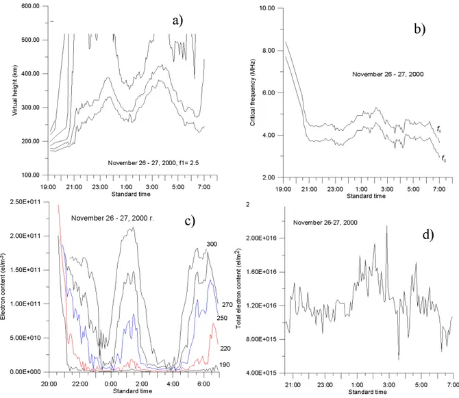
Fig. 1. Plots of the temporal variations of: (a) virtual heights (x-component of the ionospheric signal) corresponding to specific frequencies
of 2.5 MHz, 3.5 MHz, 4.5 MHz, 5.5 MHz, and 6.5 MHz, (b) critical frequencies of the ordinary (fo) and extra-ordinary (fx) components, (c) the electron content at series of heights h = 190 km, 220 km, 250 km, 270 km, and 300 km, (d) the total electron content below the F-layer peak.
2 Temporal behaviour of ionospheric parameters
For comparison CTIM model results and ionospheric verti-cal sounding night-time observations of TIDs in the F-region of the ionosphere were carried out from June 2000 through May 2001 by the digital multifunctional ionosonde BASIS installed at Almaty (76◦550E, 43◦150N). The night-time of
observations was chosen because a burst of the electric field was simulated in the night sector of the auroral region; in addition, the night-time mid-latitude ionosphere is charac-terised by large-scale TIDs with large amplitudes (Rice et. al., 1988; Hajkowicz, 1990; Yakovets et al., 1995). In gen-eral, the sounding was carried out during 8–10 nights per month. Ionograms were recorded every 5 min. An observa-tion run lasted about 12 h in winter and 8 h in summer, in order to eliminate periods of sunset and sunrise and to pro-vide conditions of a quasi-stationary ionosphere.
The ionograms were analysed for virtual height h0(t),
crit-ical frequency f0F(t), and N(h)-profiles. BASIS provided an accuracy of 2.5 km for h0(t) and 0.05 MHz for f
0F(t). The parameters h0(t) and f0F(t) are directly available from the routine scaling of ionograms and, therefore, these parameters are frequently used for the analysis of large ionosonde data sets. In Figs. 1a and b temporal variations of h0(t) (for the ex-traordinary component of the reflected signal) and f0F(t), re-spectively, are shown for the night of 26–27 November 2000. This night was characterised by a high level of magnetic ac-tivity (6Kp = 28+). The large magnetic storm with
sud-den commence began at 05:54 UT on 26 November 2000 and lasted for several days. These plots reveal periodical varia-tions of the parameters considered. During a significant part of the measurements conducted, similar wave structures were visible in the h0(t) variations, observed throughout the entire
night. However, corresponding f0F(t) variations were less clearly discernible, as one may see in Fig. 1. The amplitudes
Ya. F. Ashkaliev et al.: Comparison of travelling ionospheric disturbance measurements 1033
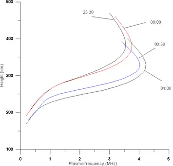
Fig. 2. Plasma frequency height profiles at 23:30, 00:00, 00:30, and
01:00 Almaty standard time for 26–27 November 2000.
of the h0(t) and f0F(t) variations changed from night to night, but these variations were almost in antiphase. From the set of h0(t) there is also evidence of downward phase propaga-tion of observed waves. Millward et al. (1993) parameterised TIDs in the CTIM model by examining several quantities: hmF, NmF, and the vertical N(h)-profiles. In order to com-pare model results and the present experimental results, we converted the ionograms into N(h)-profiles by using the accu-rate method of Titheridge (1985). Variations of the electron content at specific altitudes and total electron content below the F-layer peak were computed from N(h)-profiles. Exam-ples are plotted in Figs. 1c and 1d, respectively. Figure 2 presents a sequence of the plasma frequency height profiles for the same observation on 26–27 November 2000. Taking into account that the plasma frequency (fp) is related to the
electron content N through N = 1.24 · 104f2(where f is expressed in MHz and N in el/cm3), the plasma frequency height profiles can be easily transformed into N(h)-profiles. Millward et al. (1993) have shown that AGWs generated by the auroral events can be considered as neutral atmosphere pressure waves, so that they may be directly characterised by changing heights of fixed pressure levels in the thermo-sphere. Considering plasma vertical oscillations when an AGW was passing overhead, Rishbeth (1995) concluded that the height of a certain “cell” of plasma with constant electron density tends to follow a level of constant atmospheric pres-sure. Thus, the virtual height variations of specific sound-ing frequencies may serve as a sensitive indicator of AGWs propagating through the thermosphere.
Comparing Figs. 1a and 2 it can be seen that the iono-sphere is lifted by the positive pressure surge in the AGW, with the electron density in the F-layer peak being decreased
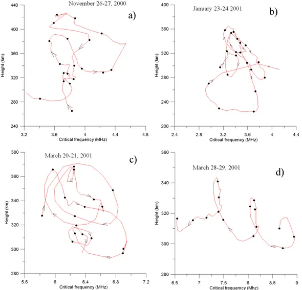
and the F-layer thickness increased at the upper position of the layer. The informative picture of behaviour of the F-layer in the course of the AGWs passing over a measurement site can be obtained if temporal variations of the height of the F-layer peak (hmF) and its critical frequency (fcr) are
plotted as a hodograph. Figure 3 shows typical examples of hodographs where adjacent points are separated by an inter-val of 30 min and arrows indicate the direction of running the process. Every hodograph presents several periods of the hmF and fcrvariations. In spite of their different forms,
most hodographs have some common features. An irregular hodograph is shown in Fig. 3a. All other hodographs demon-strate elliptically polarized trajectories with clockwise rota-tion. The eccentricity of the ellipses varies from event to event (for example, hodographs shown in Fig. 3c are almost circularly polarized), but the tilt of the main axis lies in a narrow angular range. Figure 3d shows the result of a su-perposition of the hmF and fcrvariations caused by passing
AGWs and a linear trend of these parameters in the course of the measurements. The eccentricity of the ellipse and the tilt of the main axis are defined by a phase difference between hmF and fcrvariations and the ratio of variation magnitudes.
Phase differences were estimated comparing the time series of hmF and fcr. Figure 4 shows the distribution of the phase
difference. It is evident that practically all events fall into an interval of 100◦–180◦, corresponding to a right-hand po-larisation of hodographs. Such a result shows that hmF and
fcrvariations are not in antiphase but the maximum in hmF
lags behind the minimum in fcr, and the minimum in hmF
lags behind and the maximum in the fcr. From Fig. 3 it is
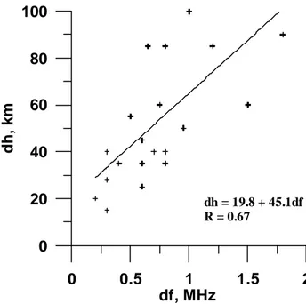
clear that there is a connection between amplitudes of hmF and fcr variations. Figure 5 illustrates the relation between
the peak-to-peak amplitudes of hmF and fcr variations (dh
and df ). A general trend towards an increase of dh with df is seen, but the data points are scattered and the correla-tion coefficient only reaches 0.67. However, in spite of con-siderable dispersion, there is the possible linear relationship
dh =19.8 + 45.1 · df .
Recently, variations in total electron content (TEC) along the line of sight from a ground-based receiver to a GPS satel-lite have been studied. Therefore, it is of principal interest to compare these results with other techniques, and, therefore, to estimate whether TID can, in principle, be seen by satel-lite techniques as well. However, the data presented in this study do not allow one to measure TEC above the F-layer peak; only measurements below it are possible. However, it will be shown later that the F-region below the F-layer peak gives the main contribution to TEC variations caused by TID. Thus, to simulate TID measurements by a satellite, TEC below the F-layer peak was computed and the results are presented in Fig. 1d. It can be seen that the same periodic structure presents in the TEC record, but the long period vari-ation (T = 4.7 h) is hardly visible on the background of short period variations. The reason for that is as follows: from the delay of the same phase of TID between various altitudes we estimated a vertical wavelength of λz ≈1400 km. This is
1034 Ya. F. Ashkaliev et al.: Comparison of travelling ionospheric disturbance measurements
Fig. 3. Typical examples of hodograph show the time evolution of the hmF versus fcr.
the passage of the AGW lifts and descends the whole F-layer practically in phase. A small decrease in TEC in the upper part of the F-layer below the layer peak that should be caused by the decrease in the NmF is compensated by increasing the layer thickness, leading to small variations of TEC.
3 Wave amplitude height profiles
It is known (Hines, 1960) that the upward energy flux of the AGWs remains constant in the nondissipative atmosphere. The wave amplitude increases with height, because the up-ward travelling wave propagates into a region of exponen-tially decreasing density of the atmosphere.
Clearly, this increase cannot be maintained indefinitely. At thermospheric altitudes, processes of dissipation, such as molecular viscosity, begin to compete with growth of the wave amplitude, leading to a maximum in the amplitude height profile. It seems that the altitude of the maximum am-plitude of the AGW differs from that of the TID maximum because the electron content height profile superimposes on
the AGW amplitude height profile. Thus, it is of great im-portance for the task of TID parameterisation to study height profiles of TIDs from measured ionograms.
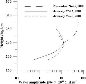
For this purpose the 5-min interval series of the electron content height profiles were used. From these profiles the temporal behaviour of the electron content at specific heights separated with an interval of 10 km was computed, as in Fig. 1c. The wave amplitude, defined as half of the peak-to-peak amplitude, was computed for each altitude. This al-lowed one to obtain the height profiles of the wave amplitude and its dependence on season and magnetic activity. The typ-ical height profiles of the TID amplitude for three nights are plotted in Fig. 6. For one of the nights the variations of iono-spheric parameters are already presented in Fig. 1. A total of 72 height profiles were analysed. The common shape of these height profiles can be approximated as a parabola, with its average thickness (defined at the level of 0.5 maximum amplitude) estimated as ∼60 km. Figure 7 shows a distribu-tion of an altitude of the TID’s maximum amplitude. The altitude of the maximum amplitude is scattered between 200
Ya. F. Ashkaliev et al.: Comparison of travelling ionospheric disturbance measurements 1035
Fig. 4. Distribution of the phase difference between the hmF and fcrvariations.
and 300 km, with the most probable value of ∼250 km (in 68.5% of all events the altitude is found between 220 and 260 km). No evident seasonal dependence of the shape and position of the height amplitude profile were noticed. The weak dependence on the magnetic activity should be pointed out. During magnetic storms, there was a tendency for the maximum amplitude, its altitude, and the thickness of the height amplitude profiles to be larger than those for the quiet magnetic conditions, as can be seen from Fig. 4.
4 Discussion
Such behaviour of F-layer parameters is remarkably consis-tent with results of a model study (Millward et al., 1993). Their Figs. 6, 7, and 8 reveal the ionospheric response to the passing AGW. This modelled response looks like the exper-imental response presented here in Figs. 1, 2, and 3. Mill-ward et al. (1993) have given an explanation of the phys-ical processes taking place in the thermosphere and iono-sphere, which were responsible for the F-layer behaviour in the course of the passing AGW over the site of observation.
The variations of the night-time ionosphere parameters during the AGW passing over the site of observation are prin-cipally caused by a redistribution of the plasma and are not due to changes in the production or loss processes. The re-distribution of the plasma is caused by the motion of the ions along the magnetic field lines. The field-aligned velocity of ions can be expressed as V k = U k + Dk, where U k is the field-aligned component of the neutral wind caused by AGW. The diffusion term Dk is the sum of the density gradient, temperature gradient, and gravity terms. Above 300 km the diffusion effect increases with height.
0
0.5
1
1.5
2
df, MHz
0
20
40
60
80
100
d
h
,
k
m
dh = 19.8 + 45.1df R = 0.67Fig. 5. Scatterplot of the peak-to-peak amplitudes of hmF variations
(dh) versus those of fcrvariations (df ).
The ion flux height profiles plotted in Fig. 7 of Millward et al. (1993) indicate the redistribution of plasma that oc-curs due to effects described above. Before the arrival of the AGW, a small downward ion flux from the plasmasphere contributes to maintaining the night-time F2-layer by pro-viding a small, continuous source of new ionisation, which compensates for the continuous loss of ionisation through re-combination and diffusion. The ion flux is strongly modified by the arriving wave. Maximum upward flux occurs near the time of the crest of the height variation wave, produc-ing an increase in hmF. The maximum flux, in this plot, lies at an altitude above the F-layer peak. Also, it can be seen that the magnitude of the flux gradient, along the magnetic field lines, is greater above the flux peak than below it. This divergence in the field-aligned flux is responsible for the de-crease in NmF, which reaches a minimum near the time of a maximum in hmF. Downward ion flux of similar magnitude and similar divergence leads to a downward shift of the lo-cation of the electron density profile. It is necessary to point out some discrepancy between the experimental and mod-eled results related to the phase difference between NmF and hmF variations. If modeled results show very small differ-ence between moments of minimum in NmF and maximum in hmF, then the experimental phase difference between these moments varies in a rather broad range from one night to an-other one. A reason for the delay of the maximum in hmF relative to the minimum in NmF is not yet understood.
The fact that the model study was performed for a sin-gle burst of electric field enhancement, while experimental records of TIDs commonly demonstrate a sequence of quasi-periodical variations of ionospheric parameters does not con-fine the results of comparison, because in practice, it is
com-1036 Ya. F. Ashkaliev et al.: Comparison of travelling ionospheric disturbance measurements
Fig. 6. Wave amplitude height profiles for three nights with
differ-ent magnetic activity: 26–27 November 2000 (6Kp=28); 22–23 January 2001 (6Kp=22); 25–26 January 2001 (6Kp=23).
mon to observe several periodical consecutive bursts in the electric field.
Thus, this study shows that the F-layer behaviour during the passage of the AGW is consistent with the results of a model study of the atmospheric and ionospheric response to a burst of enhanced electric field at high latitudes.
5 Conclusions
An experimental study of the response of the mid-latitude night-time ionosphere F-layer to passing atmospheric grav-ity waves was carried out. Ionograms were analysed for temporal variations of virtual heights taken for several fixed frequencies reflected in the ionosphere (the virtual heights of the constant electron content), critical frequency of the ionosphere F-layer, and height profiles of electron content (N(h)-profiles). A significant part of the observations showed well-defined wave structures on the h0(t) variations observed throughout the entire night, but the corresponding f0F(t) variations were less discernible. These h0(t) and f
0F(t) vari-ations were almost in antiphase. From the h0(t) there is
evidence of downward phase propagation of the observed waves. The temporal behaviour of the electron content at a series of specific heights allowed one to obtain the height profiles of the wave amplitude (el/m3). The common shape of the height profiles can be approximated by a parabola with an average thickness of ∼60 km. No evident seasonal depen-dence was visible, and the dependepen-dence on magnetic activity was weak. During magnetic storms, there was a tendency for the maximum amplitude, its altitude, and the thickness of the height amplitude profiles to be larger than those under the
200 220 240 260 280 300 320 340 360
h, km
0 10 20 30n
u
m
b
e
r
o
f
e
v
e
n
ts
Fig. 7. A distribution of an altitude of the TID’s maximum
ampli-tude.
quiet magnetic conditions. A consequence of N(h)-profiles calculated for a period of the passing wave showed them to move up and down in phase with the passing wave. As the F-layer is lifted by the positive surge in gravity wave, the electron content at the F-layer peak decreases, with the slab thickness being increased as well. Subsequently, the opposite happens as hmF falls below its equilibrium value. Such char-acteristics of the F-layer behaviour is remarkably consistent with results of a model study of the atmospheric and iono-spheric response to a short burst of enhanced ion convection at high latitudes performed with the CTIM model.
Acknowledgements. This work was performed with support of
IN-TAS through grant No. 991–1186.
Topical Editor M. Lester thanks R. Hunsucker and M. Denton for their help in evaluating this paper.
References
Fuller-Rowell, T. J., Rees, D., Quegan, S., Moffett, R. J., and Bai-ley, G. J.: Interactions between neutral thermospheric compo-sition and the polar ionosphere using a coupled ionosphere-thermosphere model, J. Geophys. Res., 92, 7744–7775, 1987. Hajkowicz, L. A.: Global study of large scale travelling ionospheric
disturbances (TIDs) following a step-like onset of auroral sub-storm in both hemispheres, Planet. Space Sci., 38, 913–923, 1990.
Hines, C. O.: Internal atmospheric gravity waves at ionospheric heights, Can. J. Phys., 38, 1441–1481, 1960.
Hocke K. and Schlegel, K.: A review of atmospheric gravity waves and travelling ionospheric disturbances: 1982–1995, Ann. Geo-physicae, 14, 917–940, 1996.
Ya. F. Ashkaliev et al.: Comparison of travelling ionospheric disturbance measurements 1037
Hunsucker, R. D.: Atmospheric gravity waves generated in the high-latitude ionosphere: A review, Rev. Geophys., 20, 293–315, 1982.
Kirchengast, G.: Elucidation of the physics of the gravity wave-TID relationship with the aid of theoretical simulations, J. Geophys. Res., 101, 13 353–13 368, 1996.
Millward, G. H., Moffet, R. J., Quegam, S., and Fuller-Rowell, T. J.: Effect of an atmospheric gravity wave on the midlatitude iono-spheric F-layer, J. Geophys. Res., 98, 19 173–19 179, 1993. Rice, D. D, Hunsucker, R. D., Lanzerotti, L. J., Crowly, G.,
Williams, P. J. S., Craven, J. D., and Frank, L.: An observation of atmospheric gravity wave cause and effect during the
Octo-ber 1985 WAGS campaign, Radio Sci., 23, 919–930, 1988. Rishbeth, H., Jenkins, B., and Moffett, R. J.: The F-layer at sunrise,
Ann. Geophysicae, 13, 367–374, 1995.
Titheridge, J. E.: Ionogram analysis with the generalised program Polan, National Geophysical Data Center, Boulder, CO USA, p. 189, 1985.
Yakovets A. F., Drobjev, V. I., and Litvinov, Yu. G.: The spatial co-herence of travelling ionospheric disturbances at mid-latitudes, J. Atmos. Terr. Phys., 57, 25–33, 1995.
Yeh K. C. and Liu, C. H.: Acoustic-gravity waves in the upper at-mosphere, Rev. Geophys. Space Phys., 12, 193–216, 1974.