HAL Id: hal-00302946
https://hal.archives-ouvertes.fr/hal-00302946
Submitted on 10 Dec 2007
HAL is a multi-disciplinary open access
archive for the deposit and dissemination of
sci-entific research documents, whether they are
pub-lished or not. The documents may come from
teaching and research institutions in France or
abroad, or from public or private research centers.
L’archive ouverte pluridisciplinaire HAL, est
destinée au dépôt et à la diffusion de documents
scientifiques de niveau recherche, publiés ou non,
émanant des établissements d’enseignement et de
recherche français ou étrangers, des laboratoires
publics ou privés.
and calcium in marine sedimentary layers
K. Bube, T. Klenke, J. A. Freund, U. Feudel
To cite this version:
K. Bube, T. Klenke, J. A. Freund, U. Feudel. Statistical measures of distribution patterns of silicon
and calcium in marine sedimentary layers. Nonlinear Processes in Geophysics, European Geosciences
Union (EGU), 2007, 14 (6), pp.811-821. �hal-00302946�
www.nonlin-processes-geophys.net/14/811/2007/ © Author(s) 2007. This work is licensed
under a Creative Commons License.
Nonlinear Processes
in Geophysics
Statistical measures of distribution patterns of silicon and calcium in
marine sedimentary layers
K. Bube, T. Klenke, J. A. Freund, and U. Feudel
Institut f¨ur Chemie und Biologie des Meeres, Carl von Ossietzky Universit¨at Oldenburg, Germany
Received: 26 July 2007 – Revised: 13 November 2007 – Accepted: 13 November 2007 – Published: 10 December 2007
Abstract. We analyze electron microscope X-ray spec-troscopy data of recent supratidal marine sediments. Sta-tistical measures are used to characterize the distribution of silicon and calcium in different layers of the sediments. We also use cluster analysis and symbolic dynamics to filter mea-surement noise and to classify different density regions. This allows to calculate characteristic patch sizes which reflect the sizes of individual clastic grains and the corresponding pore sizes. Silicon indicates the independent processes in the sed-imentation history of certain grains. Calcium is capable to monitor intrinsic early diagenetic processes of biogeochemi-cal biogeochemi-calcium mineralization of primary organic matter as doc-umented in more organized distributions with higher cluster-ing.
1 Introduction
Marine sediments are complex biogeosystems which are formed by a great variety of processes on many time and spa-tial scales. Textural and structural characteristics of a sedi-mentary sequence or even a certain layer document the act-ing processes of sedimentation (Pettijohn and Potter, 1964). The analysis of distributions of grain sizes and pores or en-sembles of components and other details of a sediment is a basic instrument in sedimentological studies (Tucker, 2001). The analysis of sediment samples gives insight into the for-mation of the sediments and therefore enables to reconstruct environmental conditions. Recently, it has been shown that biogeochemical processes involved both in the formation and in the alteration of a sediment can be monitored via care-ful analysis of sedimentary geometries (Anguy et al., 2001; Haussels et al., 2001; Morford et al., 2003; Visscher et al., 2000).
Correspondence to: U. Feudel ([email protected])
A pending problem is to identify certain processes of sed-imentation and diagenesis when analyzing different geome-tries of a sediment. A first step towards such an identifica-tion is the development of methods which yield quantitative information about sedimentary geometries. Hence the aim of this study is to provide measures on sedimentary geometries which point to physical and biogeochemical processes in a tidal environment. In this study we analyze small samples of siliciclastic tidal sediments at a millimeter scale. At this scale microorganisms form microbial mats growing on top of the inorganic matter (clastic minerals). The microbial mats form during periods of low sedimentation rates on the sediment surface. Inorganic matter can be brought in by wind. During certain flood periods the mats are buried by sedimentation. If the deposited layer is too thick, the microorganism die and the newly created sediment surface is inoculated again. Oth-erwise, microbes are capable to penetrate the surface layer and to colonize the surface again.
The chemical composition of microbial mat layers differs from other layers which were created by sedimentation pro-cesses. We want to exploit this property to distinguish differ-ent layers in the sedimdiffer-ent by the density and spatial config-uration of chemical elements. We use electron microscopy images to perform a quantitative analysis which allows us to derive unique properties for each layer. Firstly we apply an entropy measure to characterize the distribution of the el-ements. Secondly we use symbolic dynamics to calculate characteristic cluster sizes.
2 Data
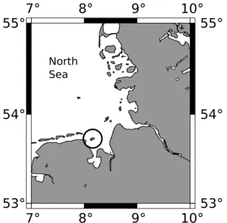
We study data samples taken from Mellum Island in the Ger-man part of the southern North Sea (see Fig. 1). The island is located in the Wadden Sea and the samples were taken from a lower supratidal area. The sediments consist of porous silici-clastic material. High biological activity during times of low
Fig. 1. The German Bight. Mellum Island is located in the middle
of the circle.
Fig. 2. Sketch of the sedimentary profile. The upper layers of the
supratidal sedimentary column represent a sequence of siliciclas-tic layers (gray parts) and intercalated microbial mats (black parts). The rectangle focuses on the section regarded in this study in detail.
sedimentation documents itself in biofilms of microbial mats. Our samples originate from the upper section of the sedimen-tary profile, which consists of fine grained quartz sand with intercalcated microbial mats and biofilms of several millime-ters thickness (Gerdes et al., 1985; Block et al., 1991). A sketch of the sediment bedding is given in Fig. 2.
Fig. 3. Working principle of the scanning electron microscope. The
X-ray backscattering is measured on a grid.
The sediment samples were prepared in small subsam-ples which were then analyzed by a scanning electron mi-croscope equipped with an energy dispersive X-ray analy-sis device (Block et al., 1991). This device measures the X-ray backscatter of the chemical elements in the probe, which were excited by an electron beam. The chemical elements are distinguished by their characteristic absorption lines. The samples are prepared in such a way that the information of the spatial distribution of the chemical elements is preserved. Figure 3 illustrates the scanning of the electron beam of the microscope. Every point of the measurement grid is pro-cessed several times. On every i-th step a number ri∈N0 is returned at point (x, y) with a certain probability which is proportional to the concentration of the chemical element under consideration. The ri are cumulated so that the
mea-surement matrix the device returns is the summation of vari-ous sampling steps. In that way, the more often the sample is scanned, the more accurately is the resulting image reflecting the underlying concentration of the chemical element. This is a consequence of the central limit theorem (Papoulis, 1984). However, the number of repetitions is limited by the time the measurement takes (about 2 min for each scan over the whole surface) and the fact that the method is not completely non-destructive. The electron beam charges the material and destroys a non-negligible amount of the sample after some measurements.
We measured densities of silicon and calcium for this test series. Those two elements were chosen since sili-con is mostly a component of inorganic matter whereas cal-cium is an important representative of organic compounds. Each measurement yields a 512×512 matrix. The surface is scanned 50 times, so that finally the measurement matrix contains the cumulated entries on the grid.
Figure 4 shows the measurement data from the micro-scope. It can be seen that the sediments consist of various layers with different characteristics. Every layer has a differ-ent abundance of chemical elemdiffer-ents and differdiffer-ent character-istic sizes of its element clusters. We calculated the layer boundaries with the help of a multiscale algorithm which searches for strong, horizontally connected, vertical gradient changes (Bube et al., 2006). In Fig. 4 the found boundaries
0 2 4 6 8 10 12 14 16 microscope counts x [mm] depth [mm] 0 0.5 1 1.5 2 x [mm] 0 0.5 1 1.5 2 depth [mm] 1 2 3 4 5 6 7 0 5 10 15 20 25 microscope counts x [mm] depth [mm] 0 0.5 1 1.5 2 x [mm] 0 0.5 1 1.5 2 depth [mm] 1 2 3 4 5 6 7
Fig. 4. Measurements from a sediment sample. The image is the
sum of 50 single measurements. The red lines are the layer bound-aries found by a layer searching algorithm. Upper panel: calcium, the numbers within the sediment plot mark the layer numbering; lower panel: silicon.
are marked with red lines. The layers were calculated for cal-cium because of its most pronounced layer structure. These layer boundaries were also taken for silicon assuming that the same layers should also be present for all elements. A cross check did not yield large deviations from this assumption.
3 Analysis
3.1 Understanding the measurement process
In the previous section we noticed that the measurement pro-cess is stochastic by nature. Therefore, we can only make statistical statements. Before we go into the surface analysis, we want to describe the measurement process in more detail. Each measurement site (x, y) scatters back a certain inten-sity of X-rays. The precise number of backscattering events and the energy of the rays is stochastic as a number of ef-fects cause the emission of X-rays, namely the Compton effect, Auger effect and the normal relaxation of the elec-trons in the atomic hull. If a certain threshold is reached, the detector emits a signal and the count at that point is incremented by one. This may be repeated several times. The probability for a response r at point (x, y) is p(x,y)(r).
We repeat the experiment N times and add the number of
0 1 2 3 4 5 counts 0 0.5 1 1.5 2 x [mm] 0 0.5 1 1.5 2 y [mm] 0 1 2 3 4 5 counts 0 0.5 1 1.5 2 x [mm] 0 0.5 1 1.5 2 y [mm]
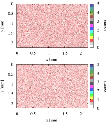
Fig. 5. Upper panel: calcium measurement data of the analysis
of glass. Lower panel: an artificial surface generated by adding exponentially distributed random numbers.
responses ri(x, y), i={1 . . . N }, the probability of the result
R(x, y)=Piri(x, y) is
p(x,y)(R) = p(x,y)(r1) ◦ · · · ◦ p(x,y)(rN), (1)
where ◦ denotes a convolution. In order to get a good estima-tion for p(x,y)(R) the number of replicates N has to be very
large. This is experimentally infeasible. In our experiment the number N =50 corresponds to the number of scans. If the surface is homogeneous, the element concentrations are constant and the fluctuations are mainly due to the atomic emission mechanisms and have the same statistics for every point. This means that the probability is spatially indepen-dent, i.e. p(x,y)(R)=p(R). Therefore, it can be estimated
from all measurement points on the surface which drastically increases the reliability. We verify this assumption by ana-lyzing glass as an amorphous material and measure the con-tents of silicon and calcium. The result is shown in the upper panel of Fig. 5. In order to model the probability density functions in terms of Eq. (1) we assume that the probability for a response is equal for each point, thus p(x,y)(r)=p(r).
This is reasonable, as the sample is homogeneous in a good approximation. Furthermore, we assume that the results ri
are uncorrelated due to the intrinsic measurement noise. This leads us to a Poisson distribution
p(r) =λ
r
r!e
−λ, (2)
10-2 100 102 104 106 0 1 2 3 p(r) r 10-2 100 102 104 106 0 1 2 3 p(r) r
Fig. 6. The dots mark the mean frequency of responses for a
sin-gle scan over the glass sample. We averaged over 50 iterations. The error bars denote the standard deviation. The solid line indi-cates the frequency calculated from a Poisson distribution with λ estimated as the mean of the measured glass data (λCa=0.0077 and
λSi=0.0455). The upper panel displays the results for calcium, the
lower one for silicon.
The parameter λ can obviously be easily calculated from the data. Therefore, we are now able to generate artificial sur-faces with the same properties as the homogeneous samples. We generate a 512×512 (the same size as the original mea-surement) matrix with natural numbers distributed according to Eq. (2). The distribution parameter λ is calculated as the mean of the 50 single measurements from the glass sample. The result is shown in Fig. 6. It matches very well the exper-imental result.
To mimic the real measurement process we generate 50 such 512×512 measurement matrices possessing the same distribution and add their entries as the cumulated values. An example is shown in the lower panel of Fig. 5. The density distribution of the resulting artificial measurement matrix is plotted in comparison to the measured glass sample in Fig. 7. Also shown in that figure is the result from a set of Poisson
101 102 103 104 105 106 0 1 2 3 4 5 p(r) r 100 101 102 103 104 105 0 2 4 6 8 10 12 14 p(r) r
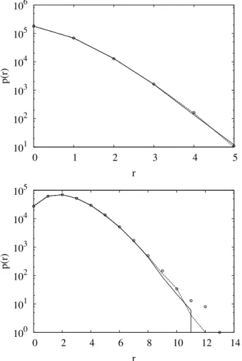
Fig. 7. Frequency of the measurement responses integrated over
50 scans. The circles mark the integrated responses measured on a glass sample, the solid line indicates the result simulated by in-tegrating over 50 Poisson distributed random surfaces, the dashed line marks the result from a single random surface with λ estimated from the integrated glass data. Upper panel: calcium, lower panel: silicon.
distributed random numbers with λ calculated directly from the measured data. Both results match equally well.
3.2 Probability analysis
In many applications one is interested in quantifying how clustered an entity which was measured on a two-dimensional grid is. A possibility for such a quantification is to assume a homogeneous distribution and calculate the deviation from this assumption. In our particular case a ho-mogeneous distribution of chemical elements on the surface plane is characterized by a Poissonian distribution of the de-tector responses as we have shown in the previous section. A structured surface violates the assumption that the average measurement is equal for every pixel and thus will yield a distribution different from a Poissonian.
When measuring data from sediments the probability for a response is not homogeneous over the sample, but spa-tially variant depending on the distribution of chemical el-ements in the sample (see Fig. 4). The probability to mea-sure a response, e.g. for silicon, is much higher at locations with quartz grains than at locations with clay. The differ-ence in terms of information between the homogeneous case and the structured case can be measured by the Kullback-Leibler (KL) divergence (also called Kullback-Kullback-Leibler dis-tance) (Kullback and Leibler, 1951), which is given by
k(p, q) =X
x
p(x) log2p(x)
q(x). (3)
q(x) is the a priori probability and p(x) the a posteriori
prob-ability. In our case the a priori probability is given by the assumption that every element is distributed homogeneously. Thus q(x) can be estimated by a Poisson distribution with the same average as the sediment measurement. p(x) is the probability which is estimated from the sediment sample.
As some a priori events are very rare and do not occur in numerical experiments we take recourse to Laplace’s succes-sor rule (Laplace, 1819)
p(x) = nx+1
N + M, (4)
where nx is the number of measurements with the
re-sult x, N is the total number of measurements and M is the number of bins in which we sort the measurements, i.e. x∈{1, 2, . . . , M}. Notice that the denominator is mod-ified to guarantee normalization, i.e.PMx=1 nx+1
N +M=1.
Figure 8 shows the distributions of the detector responses for the sediment profiles in comparison to the glass sample and Poisson distributed random numbers using the mean of the measured sediment data for the parameter λ. These distri-butions were calculated over the whole surface. We now use the KL divergence to quantify the difference between the dis-tributions in terms of information. As we have shown above, the Poisson distributed random matrices yield a rather good approximation of the homogeneously distributed elements in the glass sample (cf. Fig. 7). Their KL divergence is less than 2·10−4for both elements. The standard deviation of the KL divergence for 100 different realizations of the Poissonian surfaces is about 1%. As we have shown above, the Poisson distributed random matrices yield a rather good approxima-tion of the homogeneously distributed elements in the glass sample (cf. Fig. 7). Their KL divergence is less than 2·10−4 for both elements.
We note that due to the non-negativity of the KL diver-gence both measurement noise and sampling statistics effect a bias in the estimation: repeated measurements of the same glass probe or finite samples of the a-priori Poisson distri-bution q must necessarily result in a positive KL. The stan-dard deviation of the KL divergence for 100 different realiza-tions of the Poissonian surfaces is about 0.01 which marks the borderline between statistically non-significant (≤0.02)
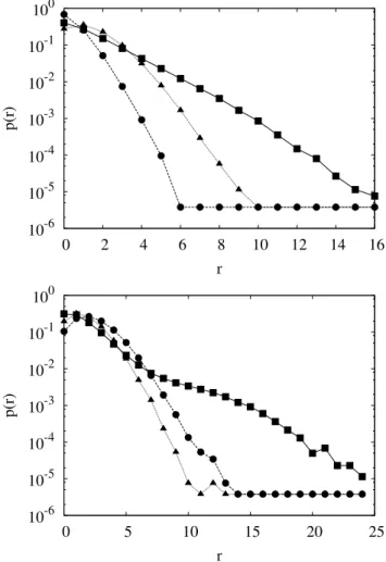
10-6 10-5 10-4 10-3 10-2 10-1 100 0 2 4 6 8 10 12 14 16 p(r) r 10-6 10-5 10-4 10-3 10-2 10-1 100 0 5 10 15 20 25 p(r) r
Fig. 8. Comparison between the sediment (solid) and the glass (long
dashes) measurements. The short dashes denote a Poissonian sur-face with the same average as the sediment sample. Upper panel: calcium, the KL divergence from the glass sample is 0.97 and from the Poissonian sample 0.17. Lower panel: silicon, the KL diver-gences are 0.40 and 0.23, respectively.
and statistically significant (>0.02) values. The KL diver-gences for the distribution shown in Fig. 8 are 0.97 for the KL divergence between the sediment calcium data and the glass sample calcium data, whereas the KL divergence be-tween sediment and Poisson distributed data for calcium is only 0.17. For the silicon data we find 0.4 (sediment – glass) and 0.23 (sediment – Poisson), respectively. It is important to note that the sediment data and the Poisson distributed random matrices possess the same mean value. Thus their comparison yields more insight than the comparison with the glass sample. That the KL divergence between sediment and glass is usually bigger than between sediment and Poisson distributed data is to a large extent due to the different mean values. Furthermore, the distribution of a homogeneous real sample depends on the material characteristics of the material chosen. If another material than glass is taken, another aver-age value of responses and thus another distribution shape
Table 1. KL divergences within the single layers. The second and
third column lists the KL divergence between the measured and an estimated Poissonian surface, the fourth and fifth the KL divergence between the measured glass sample distribution for calcium and sil-icon, respectively.
Layer Poisson Glass Ca Si Ca Si 1 0.06 0.08 0.92 0.22 2 0.08 0.14 0.32 0.28 3 0.13 0.31 0.84 0.49 4 0.47 0.05 1.87 0.87 5 0.07 0.07 0.71 0.26 6 0.11 0.24 1.41 0.53 7 0.13 0.33 0.62 0.36
has to be expected. Therefore the comparison to a randomly generated surface with the same mean value yields much more reliable results than the comparison with a homoge-neous sample of another material.
We also calculated the KL divergence for every sediment layer separately and compared it to the corresponding “layer” in the glass sample and the random matrices. The result is shown in Table 1. If compared with Fig. 4, it can be seen that the layers with large clusters have a large KL divergence to the Poisson surfaces. These are layer 3, 6 and 7 for silicon and layer 4 for calcium. The other layers are structured but do not include larger clusters which is reflected in a lower KL divergence. The layers with the lowest element densities also have a low KL divergence. For silicon this is especially layer 4 and for calcium layer 2. A few higher density regions prevent the calcium layer from being as low as the silicon layer. The KL divergences of the sediment distribution to the glass sample are generally higher than to the Poisson dis-tributed random matrices. However, these KL divergences are a bad measure to characterize the layers as sometimes clustered layers have a lower KL divergence than unclustered ones. The KL divergences of silicon layer 3 and 4 are an ex-ample for such a case.
3.3 Cluster analysis
From Fig. 4 it can be seen that the measurements are dis-turbed with noise. This is intrinsic to the X-ray backscatter-ing method as there is an amount of uncertainty involved in the backscattering of the X-rays. Therefore, it is necessary to reduce the extent of fluctuations by spatial averaging to improve the reliability of the measurements. This is justified by the fact that the grain size is typically larger than the area covered by a single measurement pixel. As one is mainly in-terested in the areas with large abundance of certain chemi-cal elements relative to the other areas we use an approach known as coarse graining from symbolic dynamics (Hao,
R11 R12 R13 R14 R21 R31 R41 R51 R52 R42 R32 R22 R23 R33 R43 R53 R54 R55 R45 R44 R34 R35 R25 R24 R15 R23 R24 R32 R33 R34 R42 R43 R44 R22
Fig. 9. Creation of an embedding vector. The neighboring points
around the center R33 are embedded. The points in the embedding vector are rank ordered afterwards.
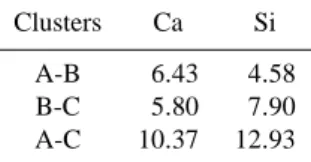
Table 2. Cluster distance measure d′for various cluster
combina-tions.
Clusters Ca Si A-B 6.43 4.58 B-C 5.80 7.90 A-C 10.37 12.93
1991; Ott, 1993; Kurths et al., 1996). Each measurement point is assigned a symbol out of a small alphabet which is associated with some distinct property of the system.
In our application it seems natural to choose some bin-ning and to sort the points into these bins. The questions that remain open are how to include the information from the neighboring points and how to choose the bin thresholds. These problems can be solved by using cluster analysis. We embed the points from the measurement grid in a vector (see Fig. 9). For each point Rx,yin the grid a corresponding
vec-tor
ξ(x, y) = (Rx−1,y−1, Rx−1,y, Rx−1,y+1, Rx,y−1, Rx,y,
Rx,y+1, Rx+1,y−1, Rx+1,y, Rx+1,y+1)
with the point itself and its next neighbors is created, yielding a 9-dimensional vector. Repeating this for every measure-ment point we end up with a set of points in a 9-dimensional vector space. As the ordering of points conveys misleading information, we rank order them. Within this 9-dimensional space it is now possible to search for clusters of points us-ing a cluster algorithm. All members of a cluster share the property that the measurement points from which its vectors are composed have similar values. This method has the ad-vantage over moving average or other coarse graining tech-niques that the binning into clusters is chosen automatically in such a way that the clusters are optimally discriminated. Furthermore all information except the spatial configuration within the grid, which is destroyed by the sorting of the points within the vectors, is preserved for the cluster search-ing.
For cluster searching we use the well known k-means al-gorithm (Hartigan, 1975; Hartigan and Wong, 1979). With this algorithm the number of clusters has to be preset. After
x [mm]
depth [mm]
0
0.5
1
1.5
2
x [mm]
0
0.5
1
1.5
2
depth [mm]
x [mm]
depth [mm]
0
0.5
1
1.5
2
x [mm]
0
0.5
1
1.5
2
depth [mm]
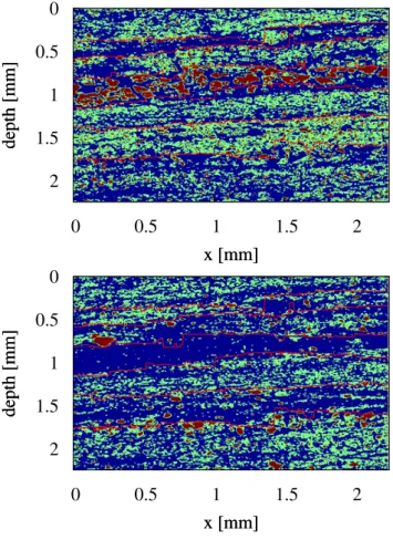
Fig. 10. Clusters calculated from the element density
measure-ments. The three colors distinguish three clusters, blue is category A, green is B and red is C. The red lines mark the layer boundaries. Upper panel: calcium; lower panel: silicon.
some trials we decided to use three clusters. Choosing more clusters does not make sense with our data sets as the found clusters are too close to each other and the information gain is not large enough to justify it. We denote the clusters with the capital letters A, B and C. A stands for the cluster with the lowest detector responses, B for intermediate values and C for the highest values. A way to measure the discriminability of the clustering is the value
d′= |µ1−µ2| |σ1+σ2|/2
, (5)
where µi is the centroid of cluster i and σi the standard
deviation of the cluster member’s distance to it (Green and Swets, 1966). Table 2 lists the values for d′calculated for our application. For comparison: if the points were Gaussian-distributed around the centroid and we put a threshold in the middle of the centroids, a short tail of both distributions lies on the opposite side of the threshold as its centroid. The d′ value would have to be 3.31 so that 95% of the distribution is on the right side of the threshold. Thus we have a satisfac-tory discriminability of the clusters. In Fig. 10 an image of
0 20 40 60 80 100 1 2 3 4 5 6 7 % layer 0 20 40 60 80 100 1 2 3 4 5 6 7 % layer
Fig. 11. Area fractions of the clusters for the various layers. The
colors are the same as in Fig. 10. Upper panel: calcium; lower panel: silicon.
the clusters found from the sediment measurement is shown. Though the layered structure is visible in Fig. 4, Fig. 10 en-ables a much more pronounced distinction of the different layers. This is due to the mentioned reduction of noise as a result of the cluster analysis, i.e. Fig. 10 is a denoised ana-logue of Fig. 4. In the fourth layer large grains of calcium can be seen, whereas in the second layer it is lacking almost completely. The others are a mixture, they differ in the struc-ture of the alternation of the different clusters. In general the structures are much clearer than in the raw measurement im-ages. Comparing the silicon and calcium image, it can be seen that the elements are complementary. In regions with a large amount of symbol C of the one element, symbol A dominates for the other. Symbol B regions act as filling and transition areas.
In our analysis we are mostly interested in how much each element is present in one layer and how it is distributed. In Fig. 11 it is shown which fraction of the area within one layer
1 10 100 1000 10000 0 0.05 0.1 0.15 0.2 0.25 0.3 frequency length [mm] Layer 1 2 3 4 5 6 7 1 10 100 1000 10000 0 0.02 0.04 0.06 0.08 0.1 0.12 0.14 0.16 frequency length [mm] Layer 1 2 3 4 5 6 7 1 10 100 1000 10000 0 0.02 0.04 0.06 0.08 0.1 0.12 0.14 frequency length [mm] Layer 1 2 3 4 5 6 7
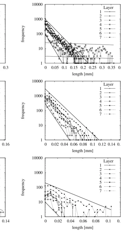
Fig. 12. Length distributions of contiguous symbols in vertical
di-rection for calcium. From top to bottom: symbol A, B, C. The thick solid lines are inserted by hand for orientation. The thick dashed line marks the corridor of the microbial mat layer. Note the differ-ent scales of the abscissa.
is covered by each symbol. In nearly all layers symbol A dominates, thus in most areas the density of the measured elements is low. However, one can also identify layers with remarkably high abundance of certain elements like layer 4
1 10 100 1000 10000 0 0.05 0.1 0.15 0.2 0.25 0.3 0.35 0.4 frequency length [mm] Layer 1 2 3 4 5 6 7 1 10 100 1000 10000 0 0.02 0.04 0.06 0.08 0.1 0.12 0.14 0.16 frequency length [mm] Layer 1 2 3 4 5 6 7 1 10 100 1000 10000 0 0.02 0.04 0.06 0.08 0.1 0.12 frequency length [mm] Layer 1 2 3 4 5 6 7
Fig. 13. Length distributions of contiguous symbols in vertical
di-rection for silicon. From top to bottom: symbol A, B, C. The thick solid lines are inserted by hand for orientation. The thick dashed line marks the corridor of the microbial mat layer. Note the differ-ent scales of the abscissa.
for calcium. From this particular layer it becomes also clear that calcium and silicon are in some sense complementary elements: when calcium content is high then the silicon con-tent is low. From this information one can conjecture that the
formation of layer 4 may be due to other mechanisms than the other layers.
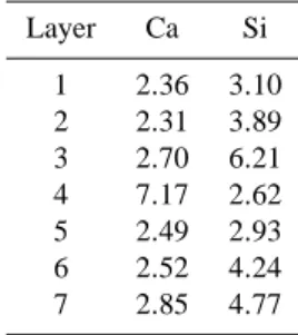
As discussed above the relative amount of material in each layer is some useful information which can be extracted by the cluster algorithm. But in general one is not only inter-ested in the overall content of elements in each layer, even more important is the spatial distribution of the elements within each layer. Usually one wants to know if the mate-rial is clustered or spread. In terms of symbolic dynamics we want to gain information on the distribution of patches from class C. A standard measure often used to address this ques-tion is the lacunarity (Mandelbrot, 1983; Allain and Cloitre, 1991; Plotnick et al., 1996). However, it did not yield satis-factory results in our application. It detected randomly scat-tered, clustered sets, but failed to return a reasonable mean patch size. Thus, in order to gain more insight into the typ-ical length scales of the different symbol clusters, we cal-culated the maximal numbers of connected pixels in vertical direction. We have chosen this direction because it is much easier to handle the rather complex boundaries of the lay-ers in vertical direction compared to the horizontal one. But the results should not depend on the direction chosen. The distribution of the lengths is shown in Figs. 12 and 13. The mean lengths for symbol C are listed in Table 3. It can be seen that the slope of the decrease in length vs. frequency is nearly the same in every layer for symbols A and B. We now consider the maximal chain lengths of the different symbols in the layers. For calcium’s symbol A the shortest lengths are found in layer 6. Their maximum length is 0.13 mm, the longest chains are in layer 7 and maximally 0.25 mm long. For symbol B the shortest length is in layer 4 (0.07 mm) and the longest in layer 2 (0.16 mm). For symbol C the short-est length is in layer 2 (0.02 mm) and the longshort-est in layer 4 (0.14 mm). The length spectrum of silicon differs substan-tially from spectra obtained for calcium. The shortest lengths are in layer 2 (0.2 mm) for symbol A, layer 4 (0.06 mm) for symbol B and again layer 4 (0.025 mm) for symbol C. The longest chains are found in layer 4 (0.35 mm) for symbol A, layer 7 (0.16 mm) for symbol B and layer 2 (0.1 mm) for symbol C. In layer 4 we get the largest contiguous calcium abundance areas. They range up to 0.14 mm. The size of the largest silicon clusters is dependent on the particular layer and lies between 0.025 mm and 0.1 mm.
4 Discussion
To tackle the problem of characterizing different layers of sediment in terms of their structures, we have used entropy measures as well as methods from symbolic dynamics. We have shown that the KL divergence between distribution functions is a good measure to characterize the homogene-ity of the distribution of chemical elements. It turned out that one has to compare the distributions obtained from the electron microscopy images of the sediment with artificially
Table 3. Mean lengths of contiguous high density clusters in
verti-cal direction. Layer Ca Si 1 2.36 3.10 2 2.31 3.89 3 2.70 6.21 4 7.17 2.62 5 2.49 2.93 6 2.52 4.24 7 2.85 4.77
created Poisson distributed random surfaces using the KL di-vergence. Due to the same mean value of the distributions the KL divergence is a reliable measure for the structuredness of the sediment surface. By contrast, the comparison with distributions in unstructured samples like glass as a refer-ence yields incorrect results which are misleading. Thus we conclude that amorphous reference samples are not a good choice when using the KL divergence. Moreover, our method of comparing the measurements to Poisson-distributed sur-faces is much simpler and adapted to the problem.
We also showed that the method is suitable to classify dif-ferent layers in the sediment. Especially layer 4 can be well isolated from the other layers. It has an eye catchingly high KL divergence in the calcium measurement which reflects the high structuredness and clustering of this chemical el-ement. Additionally, this layer exhibits a lack of silicon. The significant differences in both the calcium and the sil-icon measures enable to discriminate and to identify a buried microbial mat (layer 4) within a sequence of siliciclastic lam-inae (layers 1 to 3 and 5 to 7) (cf. Fig. 4). Silicon constitutes quartz grains of the clastic laminae. Quartz minerals are sel-dom in microbial mats, since the mats grow during times of low sedimentation rates. The organic matter is subsequently mineralised and partially replaced by calcium-minerals af-ter burial of a microbial mat grown at the surface. These calcium-minerals, however, are not formed or are unstable within the siliciclastic laminae (Kropp et al., 1997).
We further derived estimations on typical sizes of regions rich of one element or poor of it in the sediments. We achieved this estimation by coarse graining the raw measure-ment data in terms of symbolic dynamics and then studying the resulting patterns. The coarse graining sorts every mea-surement point in one of three categories: element abundance is high, medium or low. This could be expected for the sandy material in the research area. The statistical measures yield quantitative information on the porous siliciclastic layers and the alternating microbial mats. Measures on the distribution of silicon correspond to the grain sizes of the quartz minerals constituting the inorganic skeleton of the sedimentary pro-file. Individual grains of sizes up to 110 µm are indicated
(Fig. 13). This is in agreement with petrographic grain size analyses of these fine sands (mean grain sizes between 70 and 120 µm of the supratidal sediments of Mellum Island) (Gerdes et al., 1985). The deposition of individual grains is a stochastic sedimentation process of independent events by nature. The biogeochemical process of calcium miner-alization coupled with the biodegradation of microbial mats can clearly be distinguished by measures of a more homo-geneous distribution pattern which reflect a complex in situ process. The size of the resulting clusters is 120 to 140 µm in maximum. Calcium indicates clusters of authigenic high-magnesium calcite (Kropp et al., 1997). The growth of these clusters is limited by intrinsic properties, i.e. pore size or mi-crobial activity, and therefore controlled by a set of interde-pendent processes.
The measures on partially mineralized microbial mats sig-nificantly differ from those obtained for siliciclastic layers, i.e. the slope of the corridor of length distributions of con-tiguous symbol C in Fig. 12 (clusters of calcium-minerals formed during the mineralization of microbial mats) and of symbol A in Fig. 13 (microstructure of clastic grains in mi-crobial mats) are less steep than corridors of data on silici-clastic layers.
5 Conclusions
In this work we developed and applied a robust method to quantify the textural and structural homogeneity of layered sediments. The KL divergence proves to be an adequate measure for this. It enables to characterize areas of arbi-trary shape. Comparisons of sedimentary structures which are known to be homogeneous may produce misleading re-sults.
Furthermore, we introduce a way to filter measurement noise with the help of symbolic dynamics. With the fil-tered sediment profile it is then possible to extract informa-tion about characteristic patch sizes and chemical element abundance in every layer. The method can be used for mea-surements at arbitrary scale, i.e. one can apply this method to the analysis of any other two-dimensional image studied un-der the microscope as well as to the investigation of images from macroscopic measurements.
We were able to identify a buried and partially biode-graded microbial mat in a siliciclastic sequence and quantify its characteristics based on geometrical information on the concentration pattern of elements. The distribution of silicon can be regarded as indicator for physical sedimentation processes in a tidal environment. Distribution patterns of calcium indicate biogeochemical processes linked with the biodegradation of microbial mats within a siliciclastic sequence. Comparisons with samples from other areas are needed in order to give a more general interpretation on the use of elementary patterns and their relations to sedimentary processes. This is subject to ongoing research.
Edited by: H. A. Dijkstra
Reviewed by: two anonymous referees
References
Allain, C. and Cloitre, M.: Characterizing the lacunarity of ran-dom and deterministic fractal sets, Phys. Rev. A, 44, 3552–3558, 1991.
Anguy, Y., Ehrlich, R., Ahmadi, A., and Quintard, M.: On the abil-ity of a class of random models to portray the structural features of real, observed, porous media in relation to fluid flow, Cement and Concrete Composites, 23, 313–330, 2001.
Block, A., von Bloh, W., Klenke, T., and Schellnhuber, H. J.: Mul-tifractal Analysis of the Microdistribution of Elements in Sedi-mentary Structures Using Images From Scanning Electron Mi-croscopy and Energy Dispersive X Ray Spectroscopy, J. Geo-phys. Res., 96, 223–230, 1991.
Bube, K., Klenke, T., and Feudel, U.: An algorithm for detecting layer boundaries in sediments, Nonlin. Processes Geophys., 13, 661–669, 2006,
http://www.nonlin-processes-geophys.net/13/661/2006/. Gerdes, G., Krumbein, W. E., and Reineck, H.-E.: The depositional
record of sandy, versicolored tidal flats (Mellum island, southern North Sea), J. Sediment. Petrol., 55, 265–278, 1985.
Green, D. and Swets, J.: Signal detection theory and psychophysics, Wiley, New York, 1966.
Hao, B.-L.: Symbolic dynamics and characterization of complexity, Physica D, 51, 161–176, 1991.
Hartigan, J.: Clustering Algorithms, Wiley, New York, 1975. Hartigan, J. and Wong, M.: A K-Means Clustering Algorithm,
Appl. Statist., 28, 100–108, 1979.
Haussels, R., Klenke, T., Kropp, J., and Ebenh¨oh, W.: Observa-tions on the influence of pore space geometry on concentra-tion patterns and transportaconcentra-tion properties of dissolved oxygen in a bioactive sandy sediment by a lattice Boltzmann automaton model, Hydrol. Proc., 15, 81–96, 2001.
Kropp, J., Block, A., von Bloh, W., Klenke, T., and Schellnhuber, H.: Multifractal characterization of microbially induced calcite formation in recent tidal flat sediments, Sediment. Geol., 109, 37–52, 1997.
Kullback, S. and Leibler, R.: On Information and Sufficiency, An-nals of Math. Stat., 22, 79–86, 1951.
Kurths, J., Schwarz, U., Witt, A., Krampe, R., and Abel, M.: Mea-sures of Complexity in Signal Analysis, in: Chaotic, Fractal and Nonlinear Signal Processing, edited by: Katz, R., American In-stitute of Physics Conference Proceedings, vol. 375, pp. 33–54, New York, 1996.
Laplace, P.: A Philosophical Essay on Probabilities, Dover, New York, 1819.
Mandelbrot, B.: The Fractal Geometry of Nature, Freeman, New York, 1983.
Morford, J., Kalnejais, L., Martin, W., Francois, R., and Karle, I.: Sampling marine pore waters for Mn, Fe, U, Re and Mo: Modifi-cations on diffusional equilibration thin film gel probes, J. Exper. Mar. Biol. and Ecol., 285/286, 85–103, 2003.
Ott, E.: Chaos in dynamical systems, Cambridge University Press, Cambridge, 1993.
Papoulis, A.: Probability, Random Variables and Stochastic Pro-cesses, McGraw-Hill, New York, 1984.
Pettijohn, F. and Potter, P.: Atlas and glossary of primary sedimen-tary structures, Springer, Berlin, 1964.
Plotnick, R., Gardner, R., Hargrove, W., Prestegaard, K., and Perl-mutter, M.: Lacunarity analysis: A general technique for the analysis of spatial patterns, Phys. Rev. E, 53, 5461–5468, 1996.
Tucker, M.: Sedimentary Petrology, Blackwell, 2001.
Visscher, P., Reid, R., and Bebout, B.: Microscale observation of sulfate reduction: Correlation of microbial activity and lithified micritic laminae in modern marine stromatolithes, Geology, 28, 919–922, 2000.