Dissecting the Spatial Structure of Overlapping
Transcription in Budding Yeast
by
Timothy Danford
MASSACHUSEMS INS E OF TECHNOLOGyFEB 2
3
2010
LIBRARIES
Submitted to the Department of Electrical Engineering and Computer
Science
in partial fulfillment of the requirements for the degree of
Doctor of Philosophy
ARCHNVES
at the
MASSACHUSETTS INSTITUTE OF TECHNOLOGY
February 2010
@
Massachusetts Institute of Technology 2010. All rights reserved.
A uthor ... I...
Department of Electrical Engineering and Computer Science
Oct
r 19, 2009
-\
C ertified by ...
-. . . . . . . . . . . . . . .David K. Gifford
Professor
Thesis Supervisor
AAccepted by..
. . . .. .. . .' . .. . . . . . ..Terry P.
Orlando
... 7.. V.Dissecting the Spatial Structure of Overlapping
Transcription in Budding Yeast
by
Timothy Danford
Submitted to the Department of Electrical Engineering and Computer Science on October 19, 2009, in partial fulfillment of the
requirements for the degree of Doctor of Philosophy
Abstract
This thesis presents a computational and algorithmic method for the analysis of high-resolution transcription data in the budding yeast Saccharomyces cerevisiae. We begin by describing a computational system for storing and retrieving spatially-mapped genomic data. This system forms the infrastructure for a novel algorithmic approach to detect and recover instances of same-strand overlapping transcripts in high resolution expression experiments. We then apply these algorithms to a set of transcription experiments in budding yeast, Saccharomyces cerevisiae, in order to identify potential sites of same-strand overlapping transcripts that may be involved in novel forms of transcriptional regulation.
Thesis Supervisor: David K. Gifford Title: Professor
Acknowledgments
This thesis would never have been completed without the help, both personal and academic, that I received from a large number of people. Bruce Donald mentored me as an undergraduate, directed me to graduate school, and remains the smartest man I've ever met. At MIT, Ernest Frankel, Ben Gordon, Rick Young, Gerry Fink, and Tommi Jaakkola provided advice, mentorship, and careful instruction. I was lucky to have wonderful collaborators in Duncan Odom, Divya Mathur, and Sudeep Agarwala. There were also administrators without whom I never would have survived even a single semester: Jeanne Darling, Marilyn Pierce, and Janet Fischer. MIT was where I met a large number of my friends and lab-mates, including John Barnett, Shaun Mahony, Georg Gerber, Reina Riemann, Bob Altshuler, Chris Reeder, Adam Marcus, Jason Rennie. and Ted Benson. Finally, my non-MIT friends were just as instrumental in helping me survive and graduate: John Snavely, Jackson Childs, Jolene Pinder, Michelle Beaulieu, Christa Bosch, and Jason Elliott. Ale Checka and Laura Stuart deserve their own, special, acknowledgement.
Alex Rolfe has been my officemate for five years, and I've thanked my luck for each one. He's been a good friend, a close collaborator, someone to whom I can go for good and trustworthy advice, and a skilled debugger of LaTeX - in short, the best officemate a computer science student could have hoped for. Along with Alex, Robin Dowell has been a friend, collaborator, and mentor throughout the last several years of school. And, of course, David Gifford has been my advisor throughout my graduate career. He has shown endless patience, and unwavering support, over my eight years at M.I.T. The care he takes in his research, and the advice he gives to his students, speaks to his thoughtfulness and vision.
My parents, Steve and Linda, managed to sit through eight years of watching their
oldest son stumble through graduate school without ever muttering a critical word within my earshot. They supported me financially when I needed them, provided an endless stream of encouragement and help the rest of the time, and were the best co-bloggers a son could hope for. My father taught me to program and was my original
role model as a scientist; and making my mother laugh still makes me incredibly happy. I hope this thesis makes them proud.
Finally, there's Rachel: who supported me unconditionally through an expen-sive and emotionally draining experience that (at times) must have seemed as if it would never end, without whose constant encouragement and help I never would have finished, and who I love endlessly and dearly. This thesis is dedicated to her.
Contents
1 Represention and Analysis of High-Resolution Genomic Data 1.1 The Spatial Character of Modern Genomics Data . . . .. 1.2 Gene Expression and Genomic Transcription . . . ..
1.3 T hesis O utline . . . ..
2 Genomic Spatial Events Database
2.1 D esign outline . . . .. 2.1.1 Genomic coordinates as core schema . . . .. 2.1.2 Separating mapping from data . . . .. 2.2 System architecture... . . . .
2.2.1 Core schem a . . . .. 2.2.2 Microarray schema.... . . . . 2.2.3 Short-read sequencing schema . . . ..
2.3 A Dataflow Language for Biological Analysis ...
2.3.1 Discovering and representing binding events . . . ..
2.3.2 Genomic visualization . . . ...
3 Probabilistic Modeling and Segmentation of Tiling Microarrays 3.1 Prior W ork . . . ..
3.2 N otation . . . ..
3.3 Probabilistic Models of Probe Intensities . . . ..
3.4 Segmentation of Tiling Microarrays . . . ... 3.4.1 Segmentation Complexity Penalties . . . ..
3.4.2 Evaluating the SPLIT Algorithm . . . . 55
3.5 Probabilistic Models of Differential Expression from Segmented Data 57 3.5.1 Evaluating the hRMA Model . . . . 58
4 Computational Recovery of Overlapping Transcripts 63 4.0.2 Two Insights into Overlapping Transcript Detection . . . . 65
4.1 Prior W ork . . . . 67
4.2 N otation . . . . 70
4.3 An Additive Model of Transcription . . . . 72
4.4 STEREO: Reassembly of Overlapping Transcripts . . . . 73
4.4.1 Evaluating an Arrangement . . . . 75
4.4.2 Arrangement Complexity Penalties . . . . 76
4.4.3 Assumptions for Overlapping Transcript Detection . . . . 77
4.4.4 Enumerating Arrangements.. . . . . . . . 78
4.5 Performance and Testing of STEREO . . . . 79
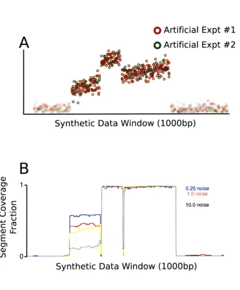
4.5.1 Synthetic D ata . . . . 81
5 Computational Detection of Overlapping Transcripts in Saccharomyces cerevisiae 85 5.1 Introduction . . . . 85
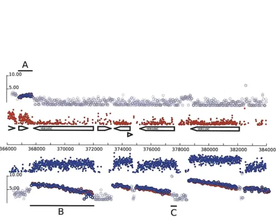
5.2 RNA cis-regulation in S288C and E1278b. . . . .. 87
5.3 SPLIT identifies expression using multiple constraints . . . . 87
5.4 STEREO assembles transcripts from expressed segments . . . . 88
5.4.1 STEREO Transcript discovery recovers appropriate SER3 and SRG1 transcripts . . . . 89
5.4.2 Identification of 1446 overlapping transcripts . . . . 90
5.4.3 Northern analysis of overlapping predictions . . . . 91
List of Figures
2-1 GSE Server/Client Structure . . . . 2-2 GSE Core Schema . . . . 2-3 GSE Microarray Schema . . . .
2-4 GSE ChIP-Seq Schema . . . .
2-5 GSE Visualizer... . . . . . . . . 2-6 Example GSEBricks Pipeline.... . . . ... 3-1 3-2 3-3 3-4 3-5 3-6 3-7 3-8 3-9
Unbiased Assessment of Transcription via Tiling Array and Segment Notation . . . . Local Flat Model ...
Local Linear Model . . . . Synthetic Segment Recovery . . . .
Microarrays
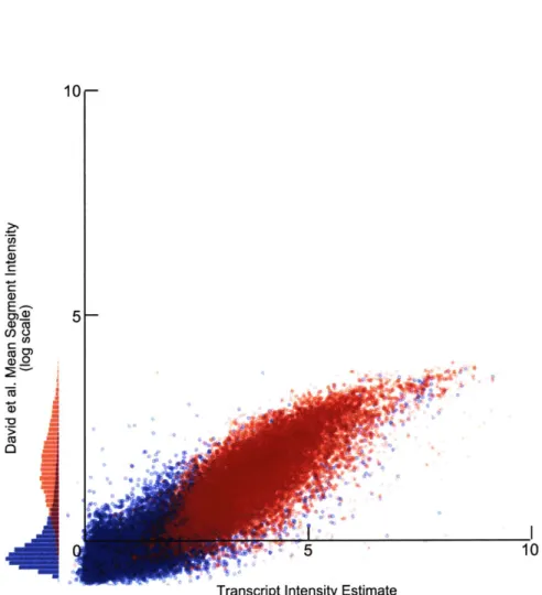
Comparison with 3rd Party Dataset: David et al. . . . . Relative Intensity Comparison: David et al. . . . . Differential Transcription in E1278b: ERG13 and PH084 Global Differential Transcription in E1278b . . . ..
4-1 Overlapping Insight #1: Additivity.. . . . ..
4-2 Overlapping Insight #2: Differential Transcription . . . . 4-3 Workflow of Transcript Reconstruction Algorithm . . . ... 4-4 STEREO Workflow Diagram . . . . 4-5 STEREO Algorithm . . . . 4-6 Pseudcode for Arrangement Enumeration . . . . 4-7 Counting arrangements under a K-maximum-overlap constraint. .
. . . . 48 . . . . 49 . . . . 59 . . . . 60 . . . . 61 . . . . 62 . . 62 83
4-8 Synthetic Transcript Reconstruction. . . . . . . . . 84
5-1 Capturing Regulatory Intergenic Transcripts Upstream of FLO11 . . 88 5-2 Transcript Reconstruction . . . . 90 5-3 Multiple Transcripts at YCR082W . . . . 92
List of Tables
4.1 Array and Transcript Notation... . . . . . . . . 71
Chapter 1
Represention and Analysis of
High-Resolution Genomic Data
The experimental design and analysis of genomic data has, in the past, often been based on gene annotations or another discrete set of units. Microarray expres-sion experiments' results are typically summarized by gene-specific intensities or values. ChIP-Chip transcription factor binding experiments are designed to probe well-defined promoter regions corresponding to individual genes, and their analysis is carried in terms of those genes. These discrete analyses were influenced by the cov-erage limitations of early microarray technologies, which had probe densities roughly equivalent to the number of genes in bacteria or yeast. Later array technologies provided genomic coverage sufficient to cover smaller genomes, but only had enough probes to tile around the start-sites of gene annotations in higher eukaryotes (human and mouse).
Biological analysis of these experiments begins with gene-based genomic data, then combines those results with other structured data sources such as protein interaction networks[28] or transcriptional regulatory networks[25]. Often these analyses look for paths, cliques, or other graph-theoretic patterns that are reflected in the original experimental dataset[9]. Even simpler analyses, based on matching experimental results against large numbers of predefined gene sets or other annotations can be used as a large-scale screening mechanism[57]. The concept of enrichment, the
over-representation of discrete units (such as genes) defined by a genomic dataset within a pre-defined collection of sets, is a central concept to much of systems-biological analysis[43].
These kinds of analyses, in terms of separate and independent units, still only give us an incomplete picture of the genome's biology. Chromatin structure, or chem-ical marks applied to histones or the DNA itself, add a second layer of information that cannot be completely inferred from the chromosomal sequence itself[36]. Genes have diverse regulatory structures, often with multiple promoters and enhancers that are located kilobases away from the annotated start of the gene's coding sequence. Gene transcripts may be spliced into different coding messages or may have alternate transcriptional forms. More recently, systematic studies have begun to show that "transcription" is not limited only to the coding regions of the genome, but widely occurs (and is prevalent, in some genomes) in the intergenic regions. These so-called "noncoding RNAs" may be functional in their own right or may carry a function through the act of their production[58].
To take a step beyond simple genes and gene-sets requires spatial analysis meth-ods. Spatial models and algorithms treat the genome as an experimental landscape, and only attempt to tie experimental results and observations back to genes or other annotations during the analysis. A spatial approach to genomic analysis identifies transcription factor binding, chromatin state or histone marks, and transcriptional ac-tivity, based on their genomic location which is determined without bias from nearby sequence annotations.
High-density microarrays and high-throughput sequencing are allowing researchers to finally measure events at high spatial resolution and across a genome-wide scale. Microarrays with probe spacings every 50 nucleotides, or even less than the width of the array's probe itself (so called tiling microarrays), are able to provide measurements across an entire chromosome from which the fine structure of biological events can be deconvolved. High-throughput sequencing technologies sample DNA fragments from an experimental population that are sequenced and mapped back to the target genome. A deconvolution process can be used to decode the locations of specific
events and biological processes along the genome from the mapped results.
Hand in hand with these novel experimental methods, researchers have created computational and statistical frameworks for their spatial analysis. Deconvolution is a popular method for finding the precise locations of biological events which we expect to have a point-like existence along the genome [50, 66]. The binding locations of transcription factors are often modeled as occurring at a single base-pair (or regions of only a few base-pairs in length). Other biological processes are expected to produce regions of activity; the interpretation of these experimental datasets often requires a statistical "segmentation" process, in which the active regions are identified and separated from the inactive or background regions. Examples of experiments which can be interpreted in this way include CGH datasets, histone density and chromatin accessibility, or high-resolution transcription datasets. These analysis methods can be used for either microarray or sequencing-based experimental results.
Segmentation-based spatial analysis methods will overlook overlapping events. Some biological phenomena cannot be understood solely as individual, independent, and non-overlapping regions. For example, transcripts may overlap due to the time-and population-averaged nature of microarray experiments time-and cell populations. If two sub-populations of cells within a biological sample are producing different scripts which cover genomic regions that are not completely disjoint, then these tran-scripts will appear on a microarray (or other experimental measurement) as overlap-ping events. Other dynamic genomic phenomena, which could be present at different locations in different cell populations, will present similar overlapping experimental signatures. Analysis of these experimental datasets should attempt to recover these coherent but overlapping regions when at all possible; otherwise, the experimenter may be led to believe that three transcripts are present instead of (for example) two, or be mistaken in the relative locations and intensities of the transcripts that are present.
In this thesis, we describe how to adapt a novel method for the analysis of tiling microarray transcription data by applying a computational to overlapping genomic regions: additive transcript re-assembly based on genomic segmentation. We also
demonstrate the use of the software system and the new tiling microarray segmen-tation and analysis framework to model a new, systematic phenomenon observable in high-resolution tiling microarray data: the presence of overlapping transcripts in budding yeast. We conclude by demonstrating how this new computational under-standing of a genomic dataset allows us to extend our underunder-standing of transcription and regulation in this same organism.
1.1
The Spatial Character of Modern Genomics
Data
Classical biology understands genomic data in terms of its component pieces - genes and proteins - and standard biological relations between them. Undirected graphs are used to model the physical interactions between proteins. Metabolic reactions that take place within the cell can be modeled as a directed, bipartite graph between reactant nodes and reaction nodes, where the directionality of the edges reflects the input/output relationships of reactants and reactions[14]. Genes are associated with reaction nodes if their corresponding protein product catalyzes that reaction. Genes are also arranged into regulatory networks, directed graph representations connecting two genes if the product of the first gene regulates the transcription of the second gene. Some functional genetics tests, such as experiments that measure genes that are lethal when deleted in pairs or genes whose expression rescues the effects of the other deletions, are represented as networks or sets-of-sets[22]. Quantitative experi-mental measurements of genes or proteins can be represented as sets which satisfy a pre-determined cutoff: for example, the set of genes whose expression exceeds some statistically-significant threshold level may be indicated as an over-expressed or up-regulated set associated with the experimental condition.
Modern genomics, in contrast to this classical understanding, represents genes in terms of their spatial location along a chromosomal sequence. Associating genes or other sequence features with their spatial coordinates along a linear chromosomal
sequence enforces a geometric understanding of the structure of the genome. Genes, promoters, enhancers, transcription factor binding sites, histone locations, accessible or inaccessible regions of the DNA, noncoding RNAs, enhancers, splicing motifs, and every other sequence features are points, regions, or intervals along a 1-dimensional space of coordinates. Consequently, a spatial understanding of genomic data requires new ways of representing, storing, and querying these geometric coordinates. One-dimensional regions are characterized by their spatial distance along the genome, and
by their spatial relationships to each other: inclusion, containment, and overlap.
These spatial relationships between sequence features are related to the functional relationships between the features. The regulatory relationship between a transcrip-tion factor and a target gene depends on the binding of the factor (that is, the locatranscrip-tion of its binding site, a sequence feature) within the promoter or enhancer for the target gene. Filtering these binding sites by measurements of the accessibility or inaccessi-bility of the surrounding DNA has been shown to improve the accuracy of regulatory relationship prediction - if a binding site is contained within an inaccessible region of DNA, then it is less likely to indicate a regulatory relationship between its binding transcription factor and any nearby gene[55, 54]. Genes themselves have a spatial structure reflected in the ordering and spacing of their exons and the relative loca-tions of sequence signals for splicing. Higher-order spatial patterns of genes along a longer chromosomal region, such as the Hox gene clusters in vertebrates whose spa-tial structure reflects the order of their activation and the ultimate patterning of the organism itself, can produce functional effects and relationships.
The treatment of genomes and chromosomes as one-dimensional spaces is itself an over-simplification. Recent experimental work has shown that genomes have higher-order three-dimensional structure. DNA wraps around histones in packed conforma-tions, and chromosomes contact each other in distinct locations and may even form loops or other forms of "secondary structure." The physical location of the chromatin within the nucleus itself (for instance, distance to the nuclear membrane) may even play a role in the regulation of genomic processes such as transcription[6].
poorly equipped for representing and storing these sorts of spatial relationships in an efficient manner. In the UCSC relational schema, different sets of gene or se-quence annotations are stored in separate table sets[31]. While this may reflect the incremental nature of the UCSC database's growth and the desire to keep separate datasets in separate locations, it also means that a query to the database which seeks
all annotations within a given region (a "spatial containment query") will be required
to touch many different tables. Even those database schema designs which present spatial coordinates in a single table, or a very limited set of tables, are often ill-suited to more complex patterns of spatial query. One prominent use of the spatial contain-ment query is to produce results which will be used to populate a genomic browser or automatic annotation mechanism. However a visual browser will present its results to the user in a manner which depends on the spatial scale of the query - the larger the scale the less detail will be shown, with more detail presented as the user "zooms in." The rules which are used to aggregate detailed high-resolution data into results suitable for visualization are sometimes difficult to encode in a simple relational ag-gregation or grouping operator. This deficiency has led to the development of special data structures that exist outside a relational database altogether, allowing multi-resolution indexing and novel spatial query types which are unsupported by standard
SQL languages.
1.2
Gene Expression and Genomic Transcription
Transcription of the genome, the process by which DNA is turned into mRNA, is an example of a biological process along the genome which requires a high-resolution spatial understanding. Transcription is the process by which DNA is turned into mRNA, the message which is ultimately translated into protein. We say that a gene is expressed if its sequence is transcribed. We measure the expression of a gene as a proxy for the presence and relative abundance of the protein for which the gene codes. This assumption, that expression is a suitable substitute for protein levels, is not completely accurate: the persistence or degradation of the protein itself, the editing,
regulation, transport, and translation of the mRNA message, and the presence of gene isoforms and chemical modifications of the protein which affect its functional status, all mediate the relationship between observed expression of a gene and the presence or functional efficacy of its encoded protein.
Experimental methods for measuring gene expression are varied in their ability to detect novel transcripts, produce quantitative information about expression levels, and to operate at high throughput rate. Before the existence of complete genome sequences to guide them, investigators used sequencing to determine the sequence of mRNAs purified from a cell population; these ESTs (or Expressed Sequence Tags) were organized into libraries and used to enumerate sets of transcripts which were produced by a given type of cell under particular experimental conditions. From these ESTs, or from complete genomic sequences available later, researchers could design probes which hybridized uniquely to a single putative transcript. These probes al-lowed the use of blots to measure the presence and to give rough relative abundance estimates for the expression of individual genes. Other techniques, such as qPCR, were developed as more accurate methods for quantitative measurement of gene ex-pression.
Gene expression measurements on a genome wide scale first became commonplace with the advent of microarray technologies. Microarrays are an experimental platform upon which thousands of probes can be simultaneously fixed; samples of genomic transcription are then processed, amplified, and labeled before being hybridized to the array's probes. Probes which show the presence of labeled sample material hybridized to their location provide an indication of the presence of the corresponding transcript. Quantitative estimates of expression are also possible from the amount of label present at a probe location.
A gene is expressed if there is a transcript produced by the cell which contains the
coding sequence of that gene (and which is, presumably, subsequently translated into protein). Transcription is itself a spatial process. Transcripts may run beyond the an-notated coding boundaries of the gene, containing the 5' and 3' UTRs (un-translated regions). Gene expression may be present as a function of a transcript spanning
mul-tiple genes simultaneously. Genes themselves may be multiply transcribed, with alter-nate promoters or variable endpoints. Transcription is a strand-specific phenomenon, so the ability to detect the direction in which a gene is transcribed (the presence of
sense and antisense transcripts) can be important for a functional understanding of
that gene's expression. Finally, transcripts themselves may occur outside the bounds of known gene annotations. Recent studies in yeast and humans have shown that sig-nificantly higher fractions of the genome are transcribed than are occupied by coding sequence annotations. Some of the transcribed regions of the genome are believed to have interactions with the expression of coding regions, or functional roles in their own right.
The first microarrays allowed expression measurements for thousands of genes simultaneously by using probes that were unique to each individual coding region. However, our spatial understanding of gene expression has shown us that only looking at gene expression gives an incomplete picture of the transcriptional activity along the genome as a whole. Gene-specific probes provide ambiguous information about the spatial nature of transcripts overlapping the probe and completely miss any tran-scripts that fall between the probes.
Tiling microarrays are designed to provide a spatial understanding of transcription along the entire genome. Microarray technologies allowing designs with large numbers of probes allow researchers to design arrays that tile an entire genomic sequencing with closely-spaced probes. The spacing of the probes provides a high spatial resolu-tion - few transcripts are small enough to remain undetected by falling between the probes, and detected transcription can be spatially localized to the nearest measured probe. High-throughput sequencing experiments (RNA-Seq) may also be used to provide measurements at a similar genomic resolution. By sequencing and mapping transcripts sampled from the experimental population, RNA-Seq can also determine the locations and extents of transcription.
Both tiling microarrays and RNA-Seq measure populations of transcripts from an experimental sample, either by averaging them (microarrays) or sampling from them (sequencing). These technologies are able to accurately detect the spatial bounds
of transcription, but they are unable to directly indicate the individual transcripts which are being measured. The computational analysis methods which have been applied to these experimental results attempt to classify transcribed regions from the surrounding background or noise, but do not attempt to reconstruct the presence, locations, or abundance of individual transcripts. This analysis is complicated by the fact that transcripts in a population may be derived from overlapping genomic regions, even on the same strand of the DNA. For example, two transcripts of a single gene which share the same end-point but start from alternate promoters will share a common suffix (3' end) but the longer transcript will have a prefix (5' end) that is not contained in the shorter transcript. These overlapping transcripts are observed as mixtures on the experimental apparatus (sequencing or microarrays), and are presented as regions of "complex" segmentation in existing computational analyes.
The goal of the second half of this thesis is to demonstrate a new computational algorithm for the spatial detection and analysis of overlapping transcripts in tiling microarray data. This algorithm will be adapted to use the output of standard segmentation-style analyses of microarray experiments, and will be performed inde-pendently of existing gene annotations or other sequence features.
1.3
Thesis Outline
Chapter 2 outlines our core platform, the Genomic Spatial Events (GSE) database, that provides the storage, query, analysis, and visualization framework for the rest of this thesis. We also outline, in the same chapter, two previously-published uses of the GSE system for analyzing genomic datasets in the same genome and between different species. Chapters 3 to 5 describe the application of a system built atop
GSE to analyze strand-senstive tiling microarrays for the detection of coding and
noncoding transcription in budding yeast. Chapter 3 describes the adaptation of a standard method for normalizing expression microarray datasets (Robust Multichip Averaging, or RMA) for use with new type of tiling microarrays. In Chapter 4, we
outline how these tiling microarrays can be used to detect a biological phenomenon, same-strand overlapping transcripts, which has not been previously examined using systematic computational methods at a global genomic level. Finally, in Chapter 5, we show how these computational techniques can be used to expand and refine the existing models of transcription and regulatory control in yeast.
Chapter 2
Genomic Spatial Events Database
Our understanding of experimental data and analysis methods from Chapter 1 has driven the development of an integrated storage and analysis system for genome-mapped sequence, annotation, and quantitative data. This chapter describes GSE, the Genomic Spatial Event database, a system to store, retrieve, and analyze several types of high-throughput microarray data. GSE handles expression datasets, ChIP-Chip data, genomic annotations, functional annotations, the results of our previously published Joint Binding Deconvolution algorithm for ChIP-Chip[50], and precom-puted scans for binding events. GSE can manage data associated with multiple species; it can also simultaneously handle data associated with multiple 'builds' of the genome from a single species. The GSE system is built upon a middle software layer for representing streams of biological data; we outline this layer, called GSE-Bricks. We show how it is used to build an interactive visualization application for ChIP-Chip data. This visualizer software is written in Java and communicates with the GSE database system over the network.
Some methods simultaneously collect hundreds-of-thousands, or even millions, of data points. Microarrays contain several orders of magnitude more probes than just a few years ago. Short-read sequencing produces raw reads whose individual experiment size is often measured in gigabytes [30]. For example, the Illumina sequencer produces single-end reads between 30-35 base pairs in length. A single lane of the reads from the sequencer may produce between 8-10 million reads, which (if we assume that
the bases are bit-packed but that a unique identifier is stored for each read) means that storing a single lane of reads will require on the order of 120 megabytes of disk space. The Illumina sequencer has eight parallel lanes, which means that every run (around three days) will produce nearly a gigabyte of raw sequence data. Those space requirements are simply for storing the simplest output of the sequencer, without ad-ditional information as to sequence quality information or mapped genomic locations. Furthermore, standard data structures for string analysis and pattern matching of-ten require O(N 2) space, where N
is the total length of the strings [1]. Storing these datasets in flat files, or in naive formats on disk, quickly becomes unwieldy as the data collection effort extends over months or years worth of data from multiple investigators and laboratories.
Combining these with massive genome annotation datasets, cross-species sequence alignments mapped on a per-nucleotide level, thousands of publicly-available microar-ray expression experiments, and growing databases of sequence motif information, and we are left with a wealth of experimental results (and large scale analyses) available to the investigator on a scale unimagined just a few years ago.
Successful analysis of high-throughput genome-wide experimental data requires careful thought on the organization and storage of numerous dataset types. The ability to effectively store and query large datasets has often lagged behind the so-phistication of the analysis techniques that are developed for that data. Many publicly available analysis packages were developed to work in smaller systems, such as yeast
[53].
Flat files are sufficient for simple organisms, but for large datasets they will not fit into main memory and cannot provide the random access necessary for a browsing visualizer.Modern relational databases provide storage and query capabilities for these vertebrate-scale datasets. Built to hold hundreds of gigabytes to terabytes of data, they provide access through a well-developed query language (SQL), network accessibility, query optimizations, and facilities for easily backing up or mirroring data across multiple sites.
how-ever, are web applications. Often these tools are the front-end interfaces to insti-tutional efforts that gather publicly-available data or are community resources for particular model organisms or experimental protocols. Efforts like UCSC's genome browser and its backing database [31], or the systems of GenBank
[3],
SGD[15],
Fly-Base [10] are all examples of web interfaces to sophisticated database systems for the storage, search, and retrieval of species-based or experiment-based data.
2.1
Design outline
2.1.1
Genomic coordinates as core schema
Our system for handling and analyzing genomic datasets is designed around a cen-tral observation: the way to integrate different experimental platforms and biological datasets at a genomic level is by establishing a common, comparable mapping of each dataset to genomic coordinates. Data structures assembled with reference to those coordinates - points, regions, and alignments, and per-base or per-bin scoring func-tions - are then manipulated and compared through a common set of one-dimensional geometric primitives such as overlap, containment, nearest-neighbor detection, and assignment based on distance metrics.
2.1.2
Separating mapping from data
The GSE system consistently separates the concepts of a dataset from its associated
mapping to a genome. This is a necessary separation for several distinct reasons:
1. Publicly-released genomes are subject to consistent updates and revisions.
Sep-arating the data itself from its mapping to a particular genome saves space and prevents the data system from storing multiple identical copies of the data for each independent genome revision.
2. Some data might not be able to be mapped directly to the genome itself examples include control spots on microarrays, or short-reads from sequencers
that are unable to be uniquely mapped to a genome. In many cases, we would still like these data to remain a coherent unit, and not be split into categories based on whether it can be mapped to a particular genome.
3. The mapping of some data (for instance, the short reads from modern
se-quencers) to a particular genome is itself an experimental process with its own sources of error. Storing the mapping separately from the data allows us to experiment with different methods for mapping or aligning arbitrary data to a genome, and provides the basis for apples-to-apples comparisons between dif-ferent alignment and mapping methods.
2.2
System architecture
Most analysis methods for genomic data can be decomposed into separate processes for data retrieval and stepwise analysis. Our system should provide a common set of modular software components, that can be composed in different ways for different analysis tasks and pipelines. The entire system should be designed to provide imme-diate visualization to the end-user, and that visualization should be built around the same components that form the core of any analysis pipeline - this way, the user can be guaranteed that the same data and analysis results which go into his or her static visualizations or dynamic figures should be the same as go into the batch analyses which are reported by the system.
The system that we describe here bridges the gap between the web applications that exist for large datasets and the analysis tools that work on smaller datasets.
GSE consists of back-end tools for importing data and running batch analyses as well
as visualization software for interactive browsing and analysis of ChIP-Chip data. The visualization software, distributed as a Java application, communicates over the network with the same database system as the as the middle-layer and analysis tools. Our visualization and analysis software is written in Java and are distributed as desktop applications. This lets us combine much of the flexibility of a web-application interface (lightweight, no flat files to install, and can run on any major operating
system) with the power of not being confined to a web browser environment. Our system can also connect to datastreams from multiple databases simultaneously, and can use other system resources normally unavailable to a browser application.
This paper describes the platform that we have developed for the storage of ChIP-Chip and other microarray experiments in a relational database. It then presents our system for intepreting ChIP-Chip data to identify binding events using our previously published "Joint Binding Deconvolution" (JBD) algorithm[50]. Finally, we show how we can build a system for the dynamic and automatic analysis of ChIP-Chip binding calls between different factors and across experimental conditions.
Ora e:Core, MySQL:
Chip-chip, Chip-seq UCSC mirror,
Custom annotations
Web Server
Desktop Java Client
Desktop Web Client
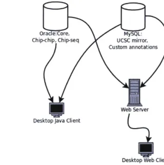
Figure 2-1: GSE is structured as either a "fat" desktop client that connects directly to the underlying database(s), or a "thin" client that can run in a web-browser.
2.2.1
Core schema
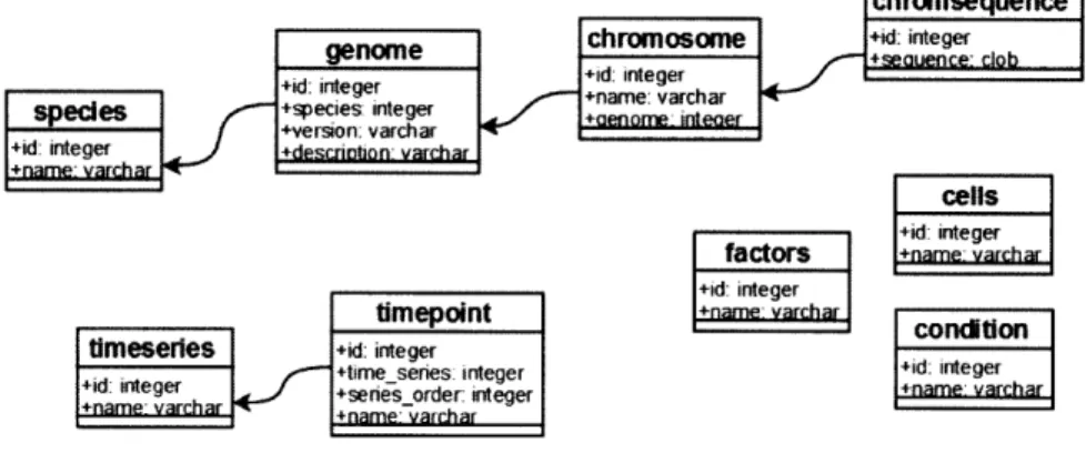
The core of our system is a database schema to represent biological data that is asso-ciated with genomic loci and assoasso-ciated metadata in a manner independent of specific genomic coordinates. Figure 2-2 shows the common metadata that all subcomponents of GSE share. We define species, genome builds, and experimental metadata that may be shared by ChIP-Chip experiments, expressiod experiments, and ChIP-Seq
experi-ments. We represent factors (e.g. an antibody or RNA extraction protocol), cell-types (tissue identifier or cell line name), and conditions as entries in separate tables.
chromsequence
enechromosome +rs ne
r+id:
integer sp m es + integer a char
+td: iteger+desrcrint on- varchar
cells
factors+id: integer +id: integer
t mepointondition
+time- mnes integer +id: integer
+id integarchars- rder integer+nm acA
Figure 2-2: CORE relational schema for the GSE System
2.2.2
Microarray schema
GSE's database system also allows multiple runs of the same biological experiment on different array platforms or designs to be so combined. Some of our analysis methods can cope with the uneven data densities that arise from this combination, and we
are able to gather more statistical power from our models when they can do so.
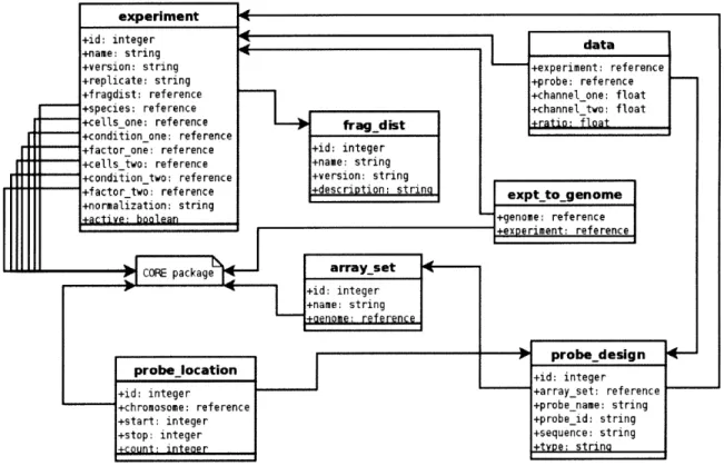
GSE stores probes separately from their genomic coordinates as shown in Figure 2-3.
Microarray observations are indexed by probe identifier and experiment identifier. A key data retrieval query joins the probe observerations and probe genomic coordinates based on probe identifier and filters the results by experiment identifier (or more typically a set of experiment identifiers corresponding to replicates of a biological experiment) and genomic coordinate. To add a new genome assembly to the system, we remap each probe to the new coordinate space once and all of the data is then available against that assembly. Since updating to a new genome assembly is a relative quick operation regardless of how many datasets have been loaded, users can always take advantage of the latest genome annotations.
In our terminology, an experiment aggregates datasets which all share the same factor, condition, and cell-type as defined in the common metadata tables. Each
Figure 2-3: MICROARRAY relational schema for the GSE System
replicate of an experiment corresponds to a single observation.
2.2.3
Short-read sequencing schema
GSE supports the storage of experimental data from high-throughput short-read
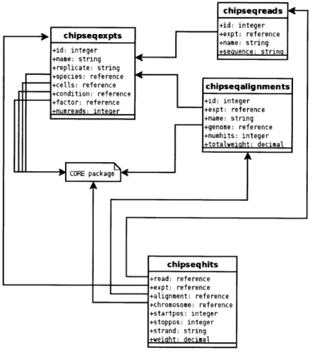
se-quencing machines in its CHIPSEQ schema. The schema for this subsystem is outlined in Figure 2-4. As with array designs in the MICROARRAY schema, the logical identity of the reads is stored separately from their alignment and their mapped locations to a particular genome. This separation of alignment from read sequence permits (a) the representation of unmapped reads in the database, (b) cleaner handling of reads which map to a genome multiple times, (c) the ability to map a dataset to the same genome multiple times (for instance, if different alignment algorithms or parameters are used), and (d) the ability to maintain mappings for a dataset to multiple genomes simultaneously.
chipsegreads4-+id: integer
Fu chipseqexpts +treference
+name: string
+id: integer
uf
i
+Aa
cal A
y
+name: string +replicate: string +species: reference
+cells: reference cutiootep n s
+condition: reference
+factor: reference o f e inte r s,
Object rgument(that i type-prameterzed in avai5) iter +numreads: t pr +expt: reference erad ite x +name: string +genome: reference +numhits: integer +totalveiaht decimal CORE package chipseqhits +read: reference +ep:reference +alignment: reference +chromosome: reference +startpos: integer +stoppos: integer +strand: string +weight: decimal
Figure 2-4: CHIPSEQ relational schema for the GSE System
2.3
A Dataflow Language for Biological Analysis
Our software system for the manipulation and analysis of biological data is called
GSEBricks. GSEBricks is a modular software package that allows the user to build
software analysis pipelines by composing smaller, reusable components. These com-ponents pass data structures representing biological objects between them in well-defined ways, and provide hooks for managing long-lived resources associated with the analysis pipeline as well as distributing the execution of the pipeline across mul-tiple threads or mulmul-tiple separate machines.
A GSEBricks module is written by extending one of three Java interfaces: Mapper,
Filter, or Expander. All of these interfaces have an 'execute' method, with a single Object argument
(that
is type-parameterized in Java 5). The Mapper and Filter ex-ecute methods have an Object(also
parameterized) as a return value. The contract ofMapper is that it produces Objects in a one-to-one relationship with its input, while a Filter may occasionally return 'null' (that is, no value). The Expander execute method, on the other hand, returns an Iterator each time it is called (although the Iterator may be empty).
Composition of GSEBricks modules is carried out by combining an instance of one of these three module classes with an existing Iterator in order to produce a new Iterator. This composition happens using one of three composition classes: MapperIterator, FilterIterator, and ExpanderIterator. A MapperIterator com-bines a Mapper with an Iterator, to produce a new Iterator; each element of the new Iterator is the result of calling Mapper on the corresponding element of the first It-erator. The FilterIterator class works the same way, although the 'null' values returned are dropped from the resulting Iterator. The Expander works by concate-nating the Iterators that result from each element of the original stream into the single new Iterator.
The second advantage to using the GSEBricks system as the basis for our visualizer is consistency. The GSE Visualizer is itself written as a modular set of custom Java Swing components, which read from GSEBricks and draw the data using the Java 2D graphics library. By building these modular graphical elements as wrappers around GSEBricks components, we are able to guarantee that the pictures from our visualizer will exactly match the data used in all our other analysis tools. This consistency is enforced because the same program code that reads and parses the data for an analysis tool is running in the visualizer itself.
This suggests the third advantage to our GSEBricks system: easy integration of analysis tools into the GSE Visualizer. Because our analysis programs are written from the same components as the visualizer, it becomes easy to simply 'plug' them into that visualizer (as dynamic options from a menu, or through interactive graphics on the visualizer itself).
The fourth advantage of the GSEBricks sysem is the easy extensibility and modi-fication of the GSE Visualizer. Its modular design lends itself to modular extensions. We have been able to quickly extend the visualizer to handle and display data such
as dynamically scanned motifs (on a base-by-base level within the visualized re-gion), automatic creation of 'meta-genes' (averaged displays of ChIP-Chip data from interactively-selected region sets), and the display of mapped reads from ChIP-PET experiments.
The final advantage of GSEBricks is the extensibility of the GSEBricks system itself. By modifying the code we use to glue the Iterators together, we can replace sequential-style list-processing analysis programs with networks of asynchronously-communicating modules that share data over the network while exploiting the parallel processing capabilities of a pre-defined set of available machines.
2.3.1
Discovering and representing binding events
Modern, high-resolution tiling microarray data allows detailed analyses that can de-termine binding event locations accurate to tens of bases. Older low-resolution ChIP-Chip microarrays included just one or two probes per gene[18, 19]. Traditional analy-sis applied a simple error model to each probe to produce a bound/not bound call for each gene rather than measurements associated with genomic coordinates[6 1]. Our Joint Binding Deconvolution (JBD) [50] exploits the dozens or hundreds of probes that cover each gene an intergenic region on modern microarrays with a complex sta-tistical model that incorporates the results of multiple probes at once and accounts for the possibility of multiple closely-spaced binding events.
JBD produces a probability of binding at any desired resolution (e.g. a per-base
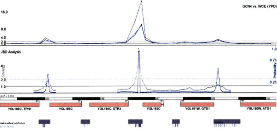
probability that a transcription factor bound that location). Figure 2-3 shows the tables that store the JBD output and figure 2-5 shows a genomic segment with ChIP-Chip data and JBD results. Unlike the raw probe observations, JBD output refers to a specific genome assembly since the spatial arrangement of the probe observations is a key input. GSE's schema also records which experiments led to which JBD analysis.
2.3.2
Genomic visualization
The GSE Visualizer is constructed as a software layer that depends on the GSEBricks library. This system provides a uniform interface to disparate kinds of data: not only ChIP-Chip data and JBD analysis, but also genome annotations, microarray expres-sion data, functional annotations, sequence alignment and orthology information, and sequence motif data. The system also handles loading the data from multiple database servers, and smoothly combining the results for any downstream program code.
There are many advantages to using a modular stream-based data system like GSEBricks for our Visualizer and analysis software. The first advantage is that it's easy for new programmers to learn how to use the system. The GSEBricks system is centered around the Java Iterator interface: this is a Java class which returns a stream of objects one at a time. GSE's visualization and GUI analysis tools depend
1.0 GCN v. WCE (YPD) 8.0 4.0 1.0 AD Anes 0.75 2.0
K025
YGL186C. TPN1 YGLI8C YGLI84C STR3 YGLI83C YGL81W. GTSI YGL18WATG1
-:-
-P
W"I I PFigure 2-5: A screenshot from the GSE Visualizer. The top track represents 'raw'
high-resolution ChIP-Chip data in yeast, and the bottom track shows two lines for the two output variables of the JBD algorithm. At the bottom are a genomic scale, a representation of gene annotations, and a custom painting of the probes and motifs from the Harbison et. al. Regulatory Code dataset. [17]
on a library of modular analysis and data-retrieval components collectively titled 'GSEBricks'. This system provides a uniform interface to disparate kinds of data: ChIP-Chip data, JBD analyses, binding scans, genome annotations, microarray ex-pression data, functional annotations, sequence alignment, orthology information,
and sequence motif instances. GSEBricks' components use Java's Iterator interface such that a series of components can be easily connected into analysis pipelines.
A GSEBricks module is written by extending one of three Java interfaces: Mapper,
Filter, or Expander. All of these interfaces have an 'execute' method, with a single Object argument which is type-parameterized in Java 5. The Mapper and Filter exe-cute methods have an Obj ect (also parameterized) as a return value. Mapper produces Objects in a one-to-one relationship with its input, while a Filter may occasionally return 'null' (that is, no value). The Expander execute method, on the other hand, returns an Iterator each time it is called (although the Iterator may be empty).
Each GSEBricks datastream is represented by an Iterator object and datas-treams are composed using modules which 'glue' existing Iterators into new sdatas-treams. Because we extend the Java Iterator interface, the learning curve for GSEBricks is gentle even for novice Java programmers. At the same time, its paradigm of building
'Iterators out of Iterators' lends itself to a Lisp-like method of functional composition, which naturally appeals to many programmers familiar with that language.
Because our analysis components implement common interfaces (eg, Iterator<Gene> or Iterator<BindingEvent>), it is easy to simply plug them into visualization or analysis software. Furthermore, the modular design lends itself to modular exten-sions. We have been able to quickly extend our visualizer to handle and display data such as dynamically re-scanned motifs (on a base-by-base level within the visual-ized region), automatic creation of 'meta-genes'[60] (averaged displays of ChIP-Chip data from interactively-selected region sets), and the display of mapped reads from ChIP-PET experiments[37].
The final advantage of GSEBricks is the extensibility of the GSEBricks system itself. By modifying the code we use to glue the Iterators together, we can replace sequential-style list-processing analysis programs with networks of asynchronously-communicating modules that share data over the network while exploiting the parallel processing capabilities of a pre-defined set of available machines.
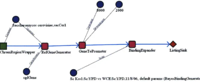
Figure 2-6 shows a screenshot from our interface to the GSEBricks system. Users can graphically arrange visual components, each corresponding to an underlying
GSE-sgdGene Sc Kss1:Sc:YPD vs WCE:Sc:YPD,11/8/06, default paams (BuyesBindhgGenerator)
BindingScanLoader loader = new BindingScanLoadero;
Genome sacCerl = Organism. findGernome ( " sacCerl " ) ;
ChromRegionWrapper chroms = new ChromRegion~rapper(sacCerl); Iterator chromItr = chroms.execute();
RefGeneGenerator rgg = new RefGeneGenerator(sacCerl, "sgdGene"); Iterator geneItr = new ExpanderIterator(rgg, chromItr);
GeneToPromoter g2p = new GeneToPromoter(8000, 2000); Iterator promItr = new HapperIterator(gZp, geneItr); BindingScan kssl = loader-loadScan(sacCerl, kssl id); BindingExpander exp = new BindingExpander(loader, kssl); Iterator bindingItr = new ExpanderIterator(exp, promItr); while (bindingItr.hasNext) ()
System. out.println(bindingItr.next ());
}
Figure 2-6: A GSEBricks pipeline to count the genes in a genome. Each box represents a component that maps objects of some input type to a set of output objects. The circles represent constants that parameterize the behavior of the pipeline. The code on the right replicates the same pipeline using Java components.
Bricks class, into structures that represent the flow of computation. This extension also allows non-sequential computational flows - trees, or other non-simply connected structures - to be assembled and computed. The interface uses a dynamic type system to ensure that the workflow connects components in a typesafe manner.
Workflows which can be laid out and run with the graphical interface can also be programmed directly using their native Java interfaces. The second half of Figure
2-6 gives an example of a code-snippet that performs the same operation using the
Chapter 3
Probabilistic Modeling and
Segmentation of Tiling Microarrays
Microarrays have been used to measure the levels of gene expression for over a decade [20]. As their use became widespread, the need to correct for sources of "obscuring variation" and to normalize the results for comparison between experiments has been a key concern for biologists. Without a correction and normalization step, probe-specific and experiment-level technical effects can obscure the interesting variation due to biological causes, and make it difficult for microarrays to inform studies of either comparative or absolute gene expression. Corrected and normalized data, however, allows the use of statistical tests to detect differential and absolute gene expression levels and to illuminate biological mechanisms of regulation and transcription. Many of the techniques which are applied to tiling or other high-density microarrays today will be extended and applied to sequencing or other high throughput techniques tomorrow.
One relatively new development in microarray technology is the advent of the
tiling microarray. Unlike earlier array designs, which sought to probe known or
puta-tive transcripts with one or more individual probes on the array, tiling arrays attempt to probe each region of the entire genome at a nearly-uniform density. Modern bi-ological understanding of transcription has shown that, in many organisms, much higher fractions of the genome are transcribed than were previously believed. Much
of that transcription is known to take place outside of confirmed gene annotations or putative open reading frames. However, microarrays which were designed to probe known gene annotations will be biased against the measurement of these non-coding transcripts. The goal of these tiling designs is fill in this blind-spot, and to allow for the unbiased measurement of transcripts throughout an entire genome.
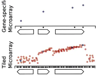
U U 0 0 CL ' 2 0 (00 -02 00% 0
Figure 3-1: Unbiased Assessment of Transcription via Tiling Microarrays Older array designs measure only the expression of annotated transcripts. Tiling mi-croarrays, by providing complete measurements along the entire genome (red probes), give a view of transcription unbiased by the annotation set.
As the total number of publicly-available microarray datasets has increased, and as the density of the microarrays themselves has deepened, efficient methods for normalization have become more important. However, many of these normalization methods were designed for earlier annotationbased nontiling microarray designs -their goal is the determination of unbiased estimates for the expression levels of individual genes which are probed by the array design. Because tiling microarrays lack this a priori assignment of probes to annotations that make traditional normalization methods possible, their analysis often requires an additional pre-processing step: the
segmentation of probes into subsets which are then considered exchangeable witnesses
to the expression of a single underlying transcript.
Modern sequencing techniques have also allowed, in the last three years, a new experimental technique for measuring transcription and other genome-wide biological
events at a high resolution. RNA-Seq has become an established method to discover the location, extent, and intensity of transcription throughout an entire genome.
3.1
Prior Work
Before any multi-experiment microarray dataset can be analyzed, it must first be normalized for inter-array comparison. Computational methods for normalization have been studied for almost as long as microarray expression data has been pro-duced
[46].
Many normalization methods are based on manufacturer-specific features of microarray design. Normalization methods for Affymetrix arrays, which contain perfect-matching and partial mis-matching (PM and MM) probe sets, can be cate-gorized by whether they use the mismatch probe information in their normalization calculation. The standard method for averaging multiple Affymetrix array experi-ments, Robust Multichip Averaging (or RMA), was developed by Irizarray, Bolstad, and Speed[5].
Other methods are designed for two-color array platforms, or for plat-forms which contain spots for "spike-in" or other artificial control values [23]. Some normalization methods attempt to reconstruct relative intensities against a baseline experiment (often the "zero" time point in a time-series experiment). Other methods depend on biological assumptions such as the constant expression of "housekeeping"' genes or the constant level of total RNA content in the sample cell population [65].The literature on the subsequent analysis, after normalization, of tiling microar-rays or other whole-genome experimental methods for measuring transcription can be divided into different categories based on the experimental platform for which the analysis method was originally designed and the method by which the locations of gene annotations are incorporated into the analysis. The supervised analyses of high-density microarrays depends on the locations of the probes relative to the gene annotations of the measured genome. These methods estimate expression values for particular genes by summarizing the observed intensities of the array probes that map within that gene's annotation (or a portion of the annotation, for splice-form specific estimation). Most methods for the unsupervised analysis for tiling microarrays, in
which gene annotations do not constrain the set of analyzed probes, were derived from older statistical models for lower-density arrays. The simplest of these methods emphasize the identification of individual "enriched" or "bound" probes [61]. When applied to a tiling or other high-density microarray, these methods were adapted to look for consecutive sequences of enriched probes that would indicate consistently high levels of expression or binding. Different approaches vary in the complexity of the model they deploy to detect bound or expressed probes. For example, a study of noncoding and intergenic expression in Mycobacterium leprae determined expression based on consecutive runs of four probes with intensities greater than 60% of the maximum normalized probe intensity score [2].
A second general approach for the analysis of tiling microarrays is derived from
methods in use for array-CGH data. These methods utilize a dynamic programming (DP) algorithm to induce a segmentation of the corresponding tiling array data. Pi-card et al. initially described a segmentation algorithm for learning constant-intensity regions in array-CGH data [48]. Their algorithm could be provided with the require-ment that segrequire-ment-level noise be constant across the entire array (homoscedastic) or could vary from segment to segment (heteroscedastic); their output produced a sequence of breakpoints, or segment boundaries, which divided the genome into re-gions of constant experimental intensity in a provably optimal way. The work of David et al. pioneered the use of the Picard segmentation method to interpret dense tiling arrays for transcription data in yeast [11, 26]. However, they had to adapt an additional statistical model for the post hoc classification of segments according to whether they were transcribed or not. Picard and his collaborators later developed a hybrid algorithm which included both of these steps in a single iterative expectation-maximization-style approach [49].
Some algorithmic approaches for identifying transcription in microarray data have relied on statistical methods for identifying "change-points" in time-series data, adapted from signal processing and econometrics literature [35]. These methods attempt to find hinges or "change points" analogous to the breakpoints induced from a segmenta-tion. Change point regression techniques can utilize statistical tests for the existence