Estimation and modeling of QT-interval adaptation to heart rate changes.

HAL Id: hal-00655140

https://hal.archives-ouvertes.fr/hal-00655140

Submitted on 20 Apr 2016

HAL is a multi-disciplinary open access

archive for the deposit and dissemination of

sci-entific research documents, whether they are

pub-lished or not. The documents may come from

teaching and research institutions in France or

abroad, or from public or private research centers.

L’archive ouverte pluridisciplinaire HAL, est

destinée au dépôt et à la diffusion de documents

scientifiques de niveau recherche, publiés ou non,

émanant des établissements d’enseignement et de

recherche français ou étrangers, des laboratoires

publics ou privés.

Estimation and modeling of QT-interval adaptation to

heart rate changes.

Aline Cabasson, Olivier Meste, Jean-Marc Vésin

To cite this version:

Aline Cabasson, Olivier Meste, Jean-Marc Vésin. Estimation and modeling of QT-interval adaptation

to heart rate changes.. IEEE Transactions on Biomedical Engineering, Institute of Electrical and

Electronics Engineers, 2012, 59 (4), pp.956-965. �10.1109/TBME.2011.2181507�. �hal-00655140�

Estimation and Modeling of QT-interval Adaptation

to Heart Rate Changes

Aline Cabasson, Olivier Meste, Member IEEE, Jean-Marc Vesin, Member IEEE

Abstract—This paper introduces a new method for QT inter-val estimation. It consists in a batch processing mode of the improved Woody’s method developed in [1]. Performance of this methodology is evaluated using synthetic data. In parallel, a new model of QT-interval dynamics behavior related to heart rate changes is presented. Since two kinds of QT response have been pointed out, the main idea is to split the modeling process into two steps: 1) the modeling of the fast adaptation, which is inspired by the electrical behavior at the cellular level relative to the electrical restitution curve, and, 2) the modeling of the slow adaptation, inspired by experimental works at the cellular level. Both approaches are based on a low-complexity autoregressive process whose parameters are estimated using an unbiased estimator. This new modeling of QT adaptation, combined with the presented QT estimation process, is applied to several ECG recordings with various heart rate variability dynamics. Its potential is then illustrated on ECG recorded during rest, atrial fibrillation episodes, and exercise. Meaningful results in agreement with physiological knowledge at the cellular level are obtained.

Index Terms—Electrocardiography (ECG), QT intervals, QT estimation, Modeling, QT adaptation.

I. INTRODUCTION

Electrocardiographic QT intervals have been widely considered as heart rate (as expressed by RR intervals) dependent [2], [3]. Nevertheless, both heart rate and autonomic nervous activity influence the QT interval dynamics [4]–[6]. The QT interval reflects the overall duration of ventricular electrical activity, and is often associated in the literature to the Action Potential Duration (APD) at the cellular level [7], [8]. The APD adaptation dynamics to abrupt changes in the cardiac period, consisting of a fast and slow responses [9]– [12], are reflected at the ECG level with QT-RR adaptation dynamics. But the combination of these two phases in the modeling of QT adaptation has been rarely addressed to date [12], [13].

In the literature, the QT response to changes in the heart period was studied during pacing-induced sudden changes [9]. It was described that 90% of QT interval adaptation to abrupt change in heart rate takes approximately 2-3 minutes. Considering the influence of preceding RR intervals, the analysis of the relationship QT/RR has been widely studied: Porta et al. [14] proposed a model to quantify the dependence Mrs. Cabasson and M. Vesin are with the Applied Signal Processing Group, Ecole Polytechnique F´ed´erale de Lausanne (EPFL), Station 11, 1015 Lausanne, Switzerland, e-mail: aline.cabasson,jean-marc.vesin@epfl.ch.

M. Meste is with the Laboratory I3S, CNRS-University of Nice-Sophia Antipolis, 2000 Route des Lucioles, 06903 Sophia Antipolis, France, e-mail: meste@i3s.unice.fr.

of the duration of ventricular repolarization with respect to the cardiac period. This study was however limited to conditions of rest, and was taken over by Almeida et al. [15]. Considering only stable heart periods, a different approach was proposed by Badilini et al. [16]. Various works investigated the case of fluctuating RR intervals, such as: El Dajani et al. [17], who proposed a model based on neural networks, Larroude et

al. [18], who studied the QT interval dynamics during atrial

fibrillation episodes, and Pueyo et al. [19], [20], who proposed a model of the QT response based on the average of previous RR intervals. This latter method makes it possible to adapt a specific model for each subject. Indeed, since the QT/RR relationship is different for each subject [21], it is important to model this relationship on an individual basis.

When one studies the trends and the variabilities of the QT and the RR intervals, two kinds of QT response to the heart period changes can be pointed out [8]–[10]: a fast phase, which takes place after a few heart beats, and a slower phase, which occurs on a longer time scale. However, no study in the literature focuses on these two adaptation phases in parallel. Most works propose a modeling of the slower phase by characterizing the evolution of the QT interval trend. In the present work, a new modeling of the QT adaptation to heart rate changes is proposed. The QT interval dynamics is considered as a weighted sum of two contributions: a fast and a slow adaptation. Both are modeled as a low-complexity autoregressive process, with unknown initial conditions, whose parameters are calculated using an unbiased estimator.

However, to perform this modeling, an accurate estimation of the QT interval is needed. Several algorithms for automated measurement have been proposed to locate QRS onsets and ends and QT interval limits. Classical segmentation methods are based on filtering the derivative of the ECG [22]–[25], or on wavelet transform [26]–[30]. The advantage of the methods based on derivative filtering lies in their robustness to variations in the morphology of the ECG waves. But the major drawback is the differentiation which is known to be sensitive to noise. In parallel, the wavelet transform has emerged as a very good segmentation tool. However when the heart rate increases, P and T waves tend to overlap and segmentation becomes impossible because these waves have similar frequency components. Recently, an indicator related to the area covered by the T wave has been proposed for the detection of the T wave [31]. The advantage of this method is its robustness against variations in the morphology of the ECG waves, but its major drawback is its sensitivity to noise. All these reasons led us to develop a new QT-interval estimation method that is presented in this paper.

0 50 100 150 200 250 300 350 400 0 0.1 0.2 0.3 0.4 0.5 0.6 0.7 Amplitude Time (ms) R

position of the maximum/2 of the first wave

The RT interval decreases with beat number

T T1 300

Fig. 1. Synthetic ECG data. This ECG has a time-varying R-T duration. This duration decreases linearly as the beat number increases. The extreme right-hand side and the extreme left-right-hand side T waves correspond, respectively, to the 1st

and the 300th

beat. SNR = − 1.1 dB.

This paper is structured as follows. Section II presents a new method of QT interval estimation in particular when the T wave undergoes significant continuous changes in shape. Section III describes the proposed modeling of QT adaptation to changes in heart rate. In Section IV, firstly the performance of the QT estimation method is evaluated and compared to those of other conventional methods using synthetic data. Secondly, the relevance of the new modeling of QT adaptation is illustrated on several real ECG recordings with various RR-trend and RR-variability dynamics: i) resting conditions, ii) atrial fibrillation episodes, iii) under controlled respiration, iv) exercise conditions. Meaningful results in agreement with the physiological knowledge at the cellular level are obtained. Finally, we conclude and suggest some future work in Section V.

II. ESTIMATION OF THEQTINTERVALS

Several algorithms for automated measurement have been proposed to locate QRS onsets and ends and QT-interval limits. Classical segmentation methods are based on filtering the derivative of the ECG [22]–[25], on wavelet transform [26]–[30], or on an indicator related to the area covered by the T wave [31]. The major drawback of these methods lies in their sensitivity to noise. A new estimation method for QT interval is presented and compared to classical estimation methods.

When the signal of interest undergoes significant continuous changes in shape, such as the T wave during exercise, batch processing is relevant. In this part, we present a method to estimate the QT intervals: a batch processing mode of the previous improved Woody’s method developed in [1]. Actually, typical time delay estimation methods such as the method developed by Woody [32], which originated from an empirical basis, has been proven as suboptimal regarding the likelihood estimation and less efficient when the number of considered beats is small. Thereby, we presented in [1] an improved version of the Woody’s method that formalizes and outperforms the previous one. These methods are based on an iterative estimation scheme for the analysis of variable latency signals, and the detection of latency by correlation between the considered signal and a template. The main difference between these methods is that the template, which is computed as the average of all beats, does not contain the considered signal in the average in the improved version of the Woody’s method. In

… … …

…

(diestimation + resulting reference waves Wi)

STEP 2 Alignment of the resulting

reference waves (Kiestimation)

…

All the delays

Æ RT intervals up a constant

…

Fig. 2. Batch processing mode of the improved Woody’s method to estimate QT intervals. After division of the original observations into M batches of 10 beats each, two steps are performed. Step 1 consists in the improved Woody’s method until convergence on each batch [1]. We obtain the estimated delays diand a resulting reference wave Wmwhich is the average of the re-aligned

waves during the improved Woody’s process. Step 2 consists in a re-alignment stage for each batch of the di. By estimating the shifts Km between the

resulting reference waves Wmof each batch, and adding this shift to those

estimated intrinsically, we get the delays for all the observations, i.e. the QT intervals up to a constant.

this part, we present a batch processing mode of the improved Woody’s method which has been proven as more efficient when the number of considered beats is small.

Successive application of two pre-processing steps provides us the position of the R waves [33]. A threshold technique applied to the high-pass filtered and amplitude-demodulated ECG, refines the estimation of the time occurrences tk of the R waves, that are roughly the R peaks locations. The high-pass filter is a 500th order FIR filter designed with a Hamming window with cutoff frequency equal to 5 Hz. Segments including each expected T wave and its previous corresponding R wave in sequence are formed by time locking the tk . The length of the segments is fixed for all beats and depends on the subject. For each heart rate, the right boundary of the segment is adjusted in order to ensure that the whole T wave is encompassed without P wave involvement. To sum up, our observations correspond to segments where all beats are aligned on the left on the R waves (see Figure 1).

Note that the number of beats per batch is chosen arbitrarily according to the mean variation of the changes of T wave in shape. If there is no variation, a batch mode is not necessary. In case of doubt, a batch method with few beats per batch (e.g. 10 beats) will always work with a cost of higher variance but a better adaptation. In the following, we create batch of 10 beats each, and apply our improved Woody’s method on each batch independently.

The global method to estimate the QT intervals, presented in Figure 2, can be split into two steps after the division of the original observations into M batches of 10 beats each:

Step 1 On each batch, processing of the improved

Woody’s method until convergence [1]. We obtain the estimated delays di (where i is the index of the beat in the considered batch) and a resulting

reference wave Wm (where m is the index of the batch) which is the average of the re-aligned waves during the improved Woody’s process.

Step 2 In step 1, given that the batches are treated

independently, the consistency is not warranted from one batch to the other one. In order to compensate the estimated delays on all observations, a stage of re-alignment of the di estimated per batch must be performed using the resulting reference waves Wm of all batches after convergence. Indeed, by estimat-ing the shifts Km between the resulting reference waves of each batch, and adding this shift to those estimated intrinsically, we get the delays for all the observations, i.e. the QT intervals up to a constant assuming that the QR intervals are stable over time. Note that the resulting reference waveform can change from one batch to another, so the estimation of the shift on the resulting reference waves for each batch must yield an absolute position. Different approaches can be used for this alignment step using temporal position of the maximum of the T wave, of the maximum divided by two in the decreasing part of the T wave, of the T-wave end based on an indicator of wave surface as proposed by Zhang et al. [31], of the T-wave end or peak based on a derivative filtering as proposed by Laguna

et al. [23]. All these approaches for this second step will be

compared in Section IV-A.

III. MODELING OF THEQTADAPTATION TO CHANGES IN

HEART RATE

In this part, we propose a new model of QT-interval dynam-ics behavior related to heart rate changes previously introduced in [34]. The QT interval response to heart period changes can be considered as a weighted sum of two contributions [10]:

• a fast adaptation, related to the variability of QT and RR intervals,

• a slow adaptation, related to the trend of QT and RR intervals.

A. Fast adaptation

The action potential duration represents the time required for a cardiac cell to achieve repolarization following a depo-larizing stimulus, and the QT interval recorded at the body surface is related to the APDs of a large number of cells, which vary from site to site in the ventricle [10], [35]. The relationship between the QT interval and the preceding TQ interval is similar to the well established restitution curve observed in isolated cells, between the APD and the preceding diastolic interval (DI) [7], [8], [10], [36]. Note that in the rest of the paper we focus on the RT and TR intervals, which correspond to QT and TQ intervals up to a constant assuming that the QR intervals are stable over time, because the R peak is easier to determine. The relationship between RT and TR (corresponding to QT and TQ intervals up to a constant) can be represented by a restitution curve at the ECG level as in Figure 3. The definition of the intervals RTn+1, T Rn. . . , is

RR increases RTn+1interval (ms) TRninterval (ms) RTn+1= g(TRn) Equilibrium point RTn+1= RR - TRn RR decreases Slope a

Fig. 3. Schematic diagram of the restitution curve at ECG level: analogy between the relationship “Action Potential Duration vs Diastolic Interval” at the cellular level, and the relationship “RT vs TR intervals” at ECG level. When an equilibrium point exists, it is possible to make a linear approximation of the restitution curve with a value a depending on the RR interval and equal to the slope of the tangent to the equilibrium point.

RRn

RTn TRn RTn+1

Beat n Beat n+1

Fig. 4. Schematic representation of normal sinus rhythm showing standard waves and definition of the RR, RT and TR intervals on two consecutive cardiac beats.

presented in Figure 4. By using the restitution curve (Figure 3), it is graphically possible to put in relation the RT intervals and the cardiac period (RR intervals). According to the definition of the cardiac intervals in Figure 4, we have:

RR(n + 1) = RT (n + 1) + T R(n + 1), (1)

or, RT(n + 1) = RR(n + 1) − T R(n + 1). (2)

For a constant heart period, i.e., a fixed RR interval, we can suppose that the TR interval remains constant. In this case, we can write equation (2) as follows:

RT(n + 1) = RR − T R(n). (3)

This latter relationship is represented in Figure 3 by the diagonal lines. The intersection of these lines with the restitu-tion curve defined by RT (n + 1) = g(T R(n)) corresponds to the equilibrium point for a fixed RR. We notice that from an equilibrium point, increase in the heart period (RR step like increase) gives rise to a fast migration to a new equilibrium point, whereas by decreasing the heart period, the new equilibrium point will be reached much more slowly since the slope of the restitution curve is greater for small RR intervals. Also, it is worth noting that if the slope of the restitution curve is greater than one, there is instability. However, the minimal and maximal physiological values of

the restitution curve are bounded by nature, so there will be emergence of a limit cycle generating alternans. When an equilibrium point exists (slope sufficiently low), it is possible to make a linear approximation of the restitution curve with a value a depending on the RR interval. It is assumed that around the equilibrium point:

RT(n + 1) = aT R(n) + b, with a > 0. (4) By developing this expression and using the definition of T R(n) in (1), we obtain a relationship between the fast adaptation of the RT intervals denoted RTf and the preceding RR intervals:

RTf(n + 1) = −aRTf(n) + aRR(n) + b. (5)

Neglecting the parameter b in a first step, which will be included in the slow adaptation process, the filter defined by relationship (5) is a high-pass filter with Z-domain response:

RTf(z) =

a

a+ zRR(z). (6)

The step response of this filter is:

RTf(z) = az (a + z)(z − 1) = α (a + z) + β (z − 1), (7) where the first term of the decomposition, α

(a+z), stands for an oscillating part, and the second term corresponds to a one lag shifted step function.

The expression (7) can explain the cellular behavior de-scribed by the restitution curve in Figure 3. Indeed, if the value of heart period (RR intervals) change abruptly, an oscillating part (related to the first term) will move around a fixed value (related to the second term). The model (6) is a high-pass filter. Note that if |a| > 1, the filter is unstable, i.e., it moves to the left side of the restitution curve and there is divergence. On the contrary, if 0 < a < 1, it is a stable high-pass filter. Then, RT intervals will be only sensitive to high-frequency components of RR intervals, i.e., to the variability of RR. The model (6) represents the cellular behavior according to the variability of heart period. Finally, the fast adaptation of the RT (or QT) response to RR changes can be defined by the relation:

RTHF(n + 1) = −a RTHF(n) + a RRHF(n), (8)

with a expected positive and less than 1, and RTHF and RRHF respectively the variability of RT and RR intervals.

The aim is then to estimate the parameter a, observing only the variability of RR intervals and using this recursive function on the variability of the RT intervals. We use an a priori range of values for a (between −0.9 and 0.9 for validation), and an initial condition RTHF(0) equal to 0. From (8), we can recursively compute RTHF, named !RTHF, for all values of n. In fact, the unknown initial condition RTHF(0) modifies RTHF(n) by adding the term RTHF(0).(−a)n−1 _{for n > 0.} For each value of a, the estimated initial condition "RTHF(0) is computed by using a least square approach. Finally, the optimal value of a is selected in such way that it minimizes the mean square error between the reconstructed "RTHF(n) =

!

RTHF(n) + "RTHF(0).(−a)n−1, and the observed one, that is:

# n

(RTHF(n) − (!RTHF(n) + "RTHF(0).(−a)n−1))2. Once the optimal value of a is computed, the variability of the RT intervals, "RTHF, is reconstructed.

B. Slow adaptation

The slow adaptation corresponds to the trend of the RT intervals, and is noted RTLF. This slow adaptation can be considered as a low-pass filtering of the preceding RR inter-vals:

RTLF(n + 1) = c RTLF(n) + RR(n), (9)

with c, positive, less than, but close to 1. In the Z-domain, this corresponds to the filter:

RTLF(z) =

1

z− cRR(z). (10)

This modeling allows to get a slow step response similar to the one obtained in the work of Franz et al. at the cellular level [10]. The value of c defines the damping factor of the exponential response [10].

Similarly to the fast adaptation, we use an a priori range of values close to 1 for c (between 0.9 and 0.999), and an initial condition RTLF(0) equal to 0. From (9), we can recursively compute RTLF, named !RTLF, for all values of n. The next step is more complex than for the fast adaptation because we will account for parameter b defined in equation (5). In that case the effect of initial condition on observations is RTLF(0).cn−1_{. For each value of c, we minimize the} following criterion:

# n

(RTLF(n) − (α!RTLF(n) + RTLF(0).cn−1+ γ))2, with respect to α, RTLF, and γ. In this criterion, α stands for a gain coefficient in the filter (10), and γ accounts for parameter b, defined in (5), and an offset, i.e., the error between the real RT interval and the observed one. Finally, the optimal value of c is selected in such way that it minimizes the mean square error between the reconstructed "RTLF(n) = ˆα.!RTLF(n) +

"

RTHF(0).cn−1_{+ ˆγ, and the observed one. Once the optimal} value of c is computed, the trend of the RT intervals, "RTLF, is reconstructed.

C. Summary of the modeling methodology

The proposed method can be summarized in a few steps: • Determination of the RR intervals,

• Estimation of the RT intervals, e.g. using a typical time delay estimation method such as the method presented in section II,

• Extraction of the trends of RT and RR intervals, using a low-pass filtering, e.g. a moving averaging filter with a Hamming window of 25 beats,

• Computation of the variabilities of RT and RR intervals by subtraction of the trends from the considered intervals, • Estimation of the oscillating part "RTHF,

• Estimation of the slow part "RTLF,

• Addition of the estimated oscillating part of the fast adaptation, and the estimated slow adaptation in order to reconstruct the entire signal "RT.

IV. RESULTS

A. Perfomance evaluation of the QT estimation method on synthetic data

1) Performance evaluation of the alignment step: In order

to find the best estimator of the shifts between resulting reference waves (i.e. the Km in the 2nd _{step of the global} method presented in Figure 2), we compare on synthetic signals different alignment approaches using:

• the temporal position of the maximum of the T wave (T-wave peak),

• the temporal position of the maximum divided by two in the decreasing part of the T wave (see example on the 1st _{synthetic T wave in Figure 1),}

• the position of the T-wave end based on an indicator of wave surface as proposed by Zhang et al. [31],

• the position of the T-wave end based on a derivative filtering as proposed by Laguna et al. [23],

• the position of the T-wave peak based on a derivative filtering as proposed by Laguna et al. [23].

The synthetic ECG data using noisy positive Gaussian func-tions is presented in Figure 1. These data have a time-varying R-T duration which decreases linearly as the beat number increases. The relative shift in the 300 Gaussian functions follows a linear progression from 0 to -50 ms. A white Gaussian noise with a standard deviation of 0.02 is added, which corresponds to a signal-to-noise ratio of −4.7 dB. In Figure 1, the extreme right-hand side and the extreme left-hand side T waves correspond respectively to the 1st_{and the 300}th beat. Parameters of Gaussian functions such as T-width have been estimated from real values. Due to the shape changes between the beats, we choose to work with batch of 10 beats each (like in real conditions). The improved Woody’s method is then applied until convergence to obtain the intra-batch delays (defined as di in Figure 2), and the resulting reference waves (defined as Wm in Figure 2) that will be used in the second step of shift estimation between each batch, i.e. the alignment process using the five estimators presented above.

Figure 5 shows the theoretical RTpeak intervals and those estimated by the global method presented in the previous section using different alignment approaches for the estimation of the shifts between resulting reference waves (Step 2 of the global method presented in Figure 2). Note that the offsets of the curves are different due to different ways for determining the interval RT: relative to the wave peak position, to the T-wave end, or to the temporal position of the maximum divided by two in the decreasing part of the T wave.

In Figure 5, we observe that the estimator of the maximum position of the T wave is very close to the theoretical RTpeak. However, the estimator based on the temporal position of the maximum divided by two presents better performance. Indeed, it is less sensitive to noisy observations than the maximum position, and has smaller variance. In parallel, we observe that

0 50 100 150 200 250 300 40 60 80 100 120 140 160 180 200 220 Beat number

RT intervals (ms) + offset RTpeak theoretical Alignment using Max Alignment using Max/2

Alignment using T_end Zhang

Alignment using T_end Laguna

Alignment using T_peak Laguna

Fig. 5. Comparison of the different alignment approaches (estimation of the shifts Kmbetween resulting reference waves of each batch: Step 2 of the

global method presented in Figure 2): the temporal position of the maximum, temporal position of the maximum divided by two in the decreasing part of the T wave, position of the T-wave end proposed by Zhang et al. [31], positions of the T-wave end and peaks proposed by Laguna et al. [23].

estimators based on the T-wave end proposed by Zhang et al. [31] or Laguna et al. [23] yield very noisy estimates of the RT intervals. The alignment method of the reference waves by detecting T-wave peak of Laguna et al. [23] has better performance than the previous ones. However, the estimator based on the position of the maximum divided by two presents the least variance.

Table I presents the values of dispersion of different align-ment approaches. The dispersion is computed as the variance of the difference between the estimated intervals and the theoretical ones after compensation of the offsets. From these values, the estimator based on the temporal position of the maximum divided by two outperforms the other approaches.

Finally in the second step of the global method, we choose to estimate the shifts between the resulting reference waves of each batch using the temporal position of the maximum divided by two in the decreasing part of the T wave.

Alignment method Dispersion

Maximum 12.50

Maximum/2 4.86

T-wave end of Zhang et al. [31] 100.74 T-wave end of Laguna [23] 50.99 T-wave peak of Laguna [23] 6.20

TABLE I

DISPERSIONS OF DIFFERENT ALIGNMENT APPROACHES(ESTIMATION OF

THE SHIFTSKmBETWEEN RESULTING REFERENCE WAVES OF EACH

BATCH: STEP2OF THE GLOBAL METHOD PRESENTED INFIGURE2). THE

DISPERSION IS COMPUTED AS THE VARIANCE OF THE DIFFERENCE BETWEEN THE ESTIMATED INTERVALS AND THE THEORETICAL ONES

AFTER COMPENSATION OF THE OFFSETS.

2) Performance evaluation of the global QT estimation method: To highlight the performance of our batch processing

mode of the improved Woody’s method, we compare it to other conventional segmentation methods [23], [26], [31], with experiments on synthetic signals.

The previous synthetic ECG data are used again (see exam-ple in Figure 1). Here the white Gaussian noise is added with a standard deviation of 0.005, which corresponds to a signal-to-noise ratio of −1.1 dB. This typical value corresponds to a

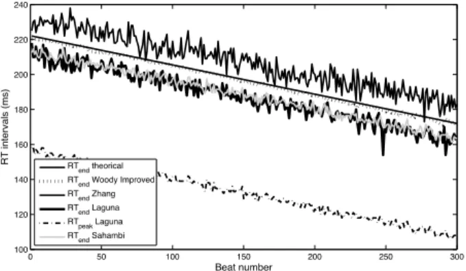
0 50 100 150 200 250 300 100 120 140 160 180 200 220 240 RT intervals (ms) Beat number RT_end theorical

RT_end Woody Improved

RT_end Zhang

RT_end Laguna

RT_peak Laguna

RT_end Sahambi

Fig. 6. Comparison of the different RT intervals estimators on synthetic data: proposed batch processing mode of the improved Woody’s method, the method of detection of the T-wave end developed by Zhang et al. [31], the method of detection of the T-wave end and of T-wave peak developed by Laguna et al. [23] and the method of detection of the T-wave end using the 23_{scale of wavelet-based method of Sahambi et al. [26].}

RT intervals estimation method Dispersion

T-wave end using

batch processing mode of the improved Woody’s method 0.31

T-wave end of Zhang et al. [31] 19.86

T-wave end of Laguna et al. [23] 11.23

T-wave peak of Laguna et al. [23] 2.26

T-wave end of Sahambi et al. [26] 3.50

TABLE II

DISPERSIONS OF THE DIFFERENTRTINTERVALS ESTIMATION METHODS.

THE DISPERSION IS COMPUTED AS THE VARIANCE OF THE DIFFERENCE

BETWEEN THE ESTIMATED INTERVALS AND THE THEORETICAL ONES

AFTER COMPENSATION OF THE OFFSETS.

standard noise level for this type of recordings. In this case, we will determine the RT intervals, but in real conditions, the QT intervals can be evaluated in the same way. Several segmentation methods are compared on these synthetic data:

• proposed batch processing mode of the improved

Woody’s method (batches of 10 beats),

• detection of the T-wave end of Zhang et al. [31], • detection of the T-wave end of Laguna et al. [23], • detection of the T-wave peak of Laguna et al. [23], • detection of the T-wave end using the 23 scale of

wavelet-based method of Sahambi et al. [26].

Figure 6 shows the RT-interval estimates for the different methods cited above. We observe that the variances of seg-mentation methods based on detecting the end or peak of the T wave are very important given the high noise sensitivity of these methods. On the other hand, the proposed batch processing mode of the improved Woody’s method shows very little variance.

Table II shows the values of the dispersion of different methods. The dispersion is computed as the variance of the difference between the estimated and theoretical RT inter-vals after compensation of the offsets. We observe the low dispersion of the proposed batch processing mode of the improved Woody’s method. It should be noted that if the noise becomes very important, some methods have a performance that degrades more quickly than others.

B. Results of the QT modeling method on real ECGs

The methodology proposed in Section III-C was applied to real ECGs. As the proposed batch processing mode of the improved Woody’s method has been proven as more efficient when the number of considered beats is small considering large variations in shape of the wave of interest, the QT estimation method described in Section II was applied and provided the RT intervals. We assume that the QR intervals are stable over time. Actually, the QR intervals represent the beginning of the depolarization, and the depolarization time on potential action is very short. So variability on this depolarization time is weaker than on repolarization time, and we hypothesized that the major variability which is observable on QT intervals comes from variability of RT intervals, i.e. of the repolarization part. Then assuming that the QR intervals are stable over time, the QR intervals were computed using an average template wave of the QR interval, and added to the RT intervals. The QT intervals were then determined. Note that in the clinical setting, the QT interval is often measured and given by the interval RT in healthy subjects. The trends of QT and RR intervals were computed using MA filtering with a Hamming window of 25 beats, and the variabilities of the QT and RR intervals were calculated by subtraction of the trends to the considered intervals.

The proposed QT modeling method was illustrated on different real ECGs in which heart rate profiles are various:

• ECG recorded at rest, for which the trend and the variability of heart rate are weak;

• ECG recorded under controlled respiration, for which the trend and the variability of heart rate are weak except during the respiration where the variability of the heart rate increases;

• ECG recorded during atrial fibrillation episodes, for which the trend of heart rate is weak while the variability of the heart rate is important;

• ECG recorded during rest and exercise, for which there is a important but continuous evolution of the heart rate with a trend which evolutes slowly then suddenly but always with a weak variability.

The choice of these different profiles of heart rate permits to test the proposed QT modeling method in different contexts. The criterion to check the success of the modeling was chosen as the Normalized Mean Square Error (NMSE) defined as:

N M SE= sum((QT − "QT) 2₎

sum(QT2₎ , (11)

where QT and "QT represent respectively the observed and the modeled QT intervals.

Then, the proposed modeling of the QT adaptation to heart rate changes combining both a fast and a slow response was applied to real ECGs, the relative parameters a and c are estimated and the average heart period determined:

• ECG recorded at rest (see Figure 7, healthy subject of the EUROBAVAR database in supine position [37]). The trend of the QT intervals is well modeled, while the variability of the modeled QT tends to the variability of

the observed one (NMSE = 1.40e−5 _{and average heart} period = 844ms);

• ECG recorded under controlled respiration in supine position (see Figure 8). As in the rest recording, the trend is well modeled, while the variability of the modeled QT tends to the variability of the observed one (NMSE = 3.21e−5 _{and average heart period = 1025ms);} • ECG recorded during atrial fibrillation episodes (see

Figure 9). The trend and the variability of the modeled QT are very close to those of the observed ones (NMSE = 6.35e−5 _{and average heart period = 705ms);}

• ECG recorded during rest and exercise on a cyclo-ergometer (see Figure 10). We observe a large modeling error when the exercise begins. Indeed, the NMSE which is equal to = 1.49e−4_{is larger than the other cases (factor} of 10). This modeling error is due to the sudden and significant drop of the RR intervals at the beginning of the exercise. The average heart period is respectively equal to 742 and 529 ms for the rest and the exercise phases In case of weak changes of heart rate trend, such as during rest or during atrial fibrillation, the heart rate is quite constant so the diagonal line on the restitution curve does not move (see Figure 3), and an equilibrium point is reached. The parameter arelative to the oscillating part in equation (8) is then constant and the QT intervals are well modeled. In case of a sudden change in the heart rate such as during exercise, the diagonal line and parameter a change, so the proposed modeling based on a constant a is not suitable for this kind of heart rate profile. In this case, a piecewise modeling process is proposed. The ECG recorded in exercise is split into two parts: rest (from the beginning of the record until the 420th _{beat in this example)} and exercise (after the 450th _{beat to the end). The transient} zone between the 420th _{and the 450}th _{beat is excluded. The} result of this piecewise QT adaptation modeling is presented in Figure 11. The NMSE of the modeling which was equal to 1.49e−4 _{considering the whole ECG, is reduced to 4.96e}−5_. On this example, we observe, especially in the exercise phase, that the variability of the QT is better preserved. Note that the estimation of the parameter a is larger for the exercise than for the resting phase. This observation has been checked on others subjects (results not provided here).

According to these results, we observe that the values of a, the slope of the tangent to the restitution curve (see Figure 3), are consistent with the average heart rate values. This observation is fully in agreement with the analysis of the restitution curve at the cellular level in Figure 3: the slope a of the tangent to the equilibrium point in the restitution curve is higher when the RR intervals decrease as during exercise. Ploting the a values in function of average RR intervals highlights a decreasing exponential relation which is consistent with the restitution curve. Indeed, for little changes in RR intervals when average RR is high, the slope a moves slightly. Only the data corresponding to the atrial fibrillation case does not fit the decreasing exponential relation. This could be explained by the large and repetitive changes in RR variability during atrial fibrillation whereas our proposed modeling assumes an almost stable RR-interval around the

equilibrium point.

In parallel, we observe that the values of the parameter c, defined in the slow adaption part in the equation (9), are representative of the low-pass filtering, i.e., close to 1 and consistent with the work of Franz et al. at the cellular level [10].

V. DISCUSSION AND CONCLUSION

In this paper, firstly we presented a new QT-interval es-timation method, a batch processing mode of the previous improved Woody’s method developed in [1]. Performance evaluation was performed on synthetic signals, and the pro-posed method in its batch processing mode outperformed the other conventional methods based on a segmentation of the T wave.

Secondly we proposed a new QT-RR adaptation modeling which provides a characterization of the QT interval adaptation dynamics in response to heart rate changes. Contrary to the previous studies, the modeling focuses both on the fast and slow QT intervals adaptations. Then, a new modeling based on two processes is proposed: at first, the oscillating part relative to the QT and RR variabilities, and secondly, the slow adaptation relative to the QT and RR trends, are modeled. The proposed fast adaptation modeling is based on the electrical behavior at the cellular level relative to the electrical restitution curve. In parallel, the slow adaptation modeling is inspired by experimental works at the cellular level too. Note that the so-called QT/RR hysteresis [20], [38] is explained by this slow adaptation. Indeed it is not only the preceding cardiac cycle that influences the QT. The history of heart rate variability contributes to QT variations.

The results on real ECG recordings in Section IV-B illustrate the feasibility of the modeling of the QT adaptation to heart rate changes. Excepted in case of an abrupt change of the heart rate as in the beginning of exercise for instance, the modeling of both trend and variability of QT intervals are satisfactory in all examples. In case of large changes in the heart rate, a piecewise modeling process is proposed, that assumes two stationary intervals in the cardiac recording. Future works can tackle this issue: instead of considering the parameter a relative to the oscillating part as constant, it would be interesting to consider it as time-varying. With this new adaptive parameter an, the modeling of the QT adaptation can be more accurate, in particular the variability. Moreover, a more realistic representation is very important since the kinetics of this parameter a has been related in some works to risk of arrhythmias, in particular to ventricular fibrillation [39], [40].

VI. ACKNOWLEDGMENTS

The authors gratefully acknowledge Dr St´ephane Bermon, PhD, and Gr´egory Blain, PhD, for providing the ECG sig-nals recorded during exercise, and Pr Connor Heneghan for providing the ECG recorded under controlled respiration.

0 100 200 300 400 500 600 700 385 390 395 400 405 410 Beat number QT i n te rv a l (m s ) observed QT modeled QT 480 500 520 540 560 580 60 RR = 845 ms a=0.035 ; c=0.966

Fig. 7. Example of modeling of the QT adaptation to RR changes on a ECG recorded at rest. NMSE = 1.40e−5_.

0 500 1000 1500 335 340 345 350 355 360 365 370 375 Beat number QT i n te rv a l (ms ) observed QT modeled QT RR = 1025 ms a=0.001 ; c=0.985 800820 840860880 900920940 9609801000

Fig. 8. Example of modeling of the QT adaptation to RR changes on a ECG recorded under controlled respiration. NMSE = 3.21e−5_.

0 50 100 150 200 250 300 350 330 335 340 345 350 355 360 365 370 375 Beat number QT i n te rv a l (m s ) observed QT modeled QT RR = 705 ms a=0.031 ; c=0.976 250 260 270 280 290 300 310

Fig. 9. Example of modeling of the QT adaptation to RR changes on a ECG recorded during atrial fibrillation episodes. Note that the trend and the variability of the modeled QT are very close to those of the observed ones. NMSE = 6.35e−5. 0 100 200 300 400 500 600 700 300 310 320 330 340 350 360 370 Beat number QT i n te rv a l (m s ) observed QT modeled QT 540 560 580 600 a=0.062 ; c=0.999

Fig. 10. Example of modeling of the QT adaptation to RR changes on a ECG recorded during exercise. We observe that the modeled QT can not really reach the observed one when the RR drop is too large in the beginning of the exercise for instance. NMSE = 1.49e−4_.

0 100 200 300 400 500 600 700 300 310 320 330 340 350 360 370 Beat number QT i n te rv a l (m s ) a=0.041 ; c=0.982 RR = 742 ms at rest a=0.290 ; c=0.989 RR = 529 ms during exercise 120 130 140 150 1 590 595 600605 610 615 620

Fig. 11. Example of modeling of the QT adaptation to RR changes on a ECG recorded during exercise. Modeling by piecewise: rest part, and exercise. Exclusion zone of model transition between the two vertical lines. NMSE = 4.96e−5.

REFERENCES

[1] A. Cabasson and O. Meste, “Time Delay Estimation: A New Insight Into the Woody’s Method,” IEEE Signal Process Lett, vol. 15, pp. 573–576, 2008.

[2] H. Bazett, “An analysis of time relations of electrocardiograms,” Heart, vol. 7, pp. 353–367, 1920.

[3] L. Fridericia, “Duration of systole in electrocardiogram,” Acta. Med. Scand., vol. 53, pp. 469–486, 1920.

[4] S. Ahnve and H. Vallin, “Influence of heart rate and inhibition of autonomic tone on the QT interval,” Circulation, vol. 65, no. 3, pp. 435–439, 1982.

[5] R. Bexton, H. Vallin, and A. Camm, “Diurnal variation of the Q-T interval influence of the autonomic nervous system,” Br. Heart J., vol. 55, no. 3, pp. 253–258, 1986.

[6] K. Browne, D. Zipes, J. Heger, and E. Prystowsky, “Influence of the autonomic nervous system on the Q-T interval in man,” Amer. J. Cardiol., vol. 50, no. 5, pp. 1099–1103, 1982.

[7] L. Arnold, J. Page, D. Attwell, C. M., and D. Eisner, “The dependence on heart rate of the human ventricular action potential duration,” Cardiovasc Res, vol. 313, pp. 547–551, 1982.

[8] W. Seed, N. Noble, R. Oldershaw, P. Wanless, A. Drake-Holland, D. Redwood, S. Pugh, and C. Mills, “Relation of human cardiac action potential duration to the interval between beats: implications for the validity of rate corrected QT interval (QTc),” Br Heart J, vol. 57, pp. 32–37, 1987.

[9] C. Lau, A. Freedman, S. Fleming, M. Malik, A. Camm, and D. Ward, “Hysteresis of the ventricular paced QT interval in response to abrupt changes in pacing rate,” Cardiovasc Res, vol. 22, pp. 67–72, 1988. [10] M. Franz, C. Swerdlow, B. Liem, and J. Schaefer, “Cycle length

dependence of human action potential duration in vivo. Effects of single extrastimuli, sudden sustained rate acceleration and deceleration, and different steady-state frequencies,” J. Clin. Invest., vol. 82, pp. 972–979, 1988.

[11] R. Gulrajani, “Computer simulation of action potential duration changes in cardiac tissue,” Computers in Cardiology, pp. 629–632, 1987. [12] E. Pueyo, Z. Husti, T. Hornyik, I. Baczk´o, P. Laguna, A. Varr´o, and

B. Rodr´ıguez, “Mechanisms of ventricular rate adaptation as a predictor of arrhythmic risk,” Am J Physiol Heart Circ Physiol, vol. 298, pp. H1577–1587, 2010.

[13] J. Halamek, P. Jurak, T. Bunch, J. Lipoldova, M. Novak, V. Vondra, P. Leinveber, M. Plachy, T. Kara, M. Villa, P. Frana, M. Soucek, V. Somers, and S. Asirvatham, “Use of a novel transfer function to reduce repolarization interval hysteresis,” J Interv Card Electrophysiol, vol. 29, pp. 23–32, 2010.

[14] A. Porta, G. Baselli, E. Caiani, A. Malliani, F. Lombardi, and S. Cerruti, “Quantifying electrocardiogram RT-RR variability interactions,” Med. Bio. Eng. Comput., vol. 36, pp. 27–34, 1998.

[15] R. Almeida, S. Gouveia, P. Rocha, E. Pueyo, J. Mart´ınez, and P. Laguna, “QT variability and HRV interactions in ECG: Quantification and reliability,” IEEE Trans. Biomed. Eng., vol. 53, pp. 1317–1329, 2006. [16] F. Badilini, P. Maison-Blanche, C. R., and P. Coumel, “QT interval

analysis on ambulatory eletrocardiogram recordings: a selective beat averaging approach,” Med. Biol. Eng. Comput., vol. 37, pp. 71–79, 1999. [17] R. El Dajani, M. Miquel, P. Maison-Blanche, and P. Rubel, “Time series prediction using parametric models and multilayer perceptrons: case study on heart signals,” ICASSP, vol. 2, pp. II 773–776, 2003. [18] C. Larroude, B. Jensen, E. Agner, E. Toft, C. Torp-Pedersen,

K. Wachtell, and J. Kanters, “Beat-to-beat QT dynamics in paroxysmal atrial fibrillation,” Heart Rhythm, vol. 3, pp. 660–664, 2006.

[19] E. Pueyo, M. Malik, and P. Laguna, “A dynamic model to characterize beat-to-beat adaptation of repolarization to heart rate changes,” Biomed Signal Process Control, vol. 3, pp. 29–43, 2008.

[20] E. Pueyo, P. Smetana, P. Caminal, A. Bayes de Luna, M. Malik, and P. Laguna, “Characterization of QT interval adaptation to RR interval changes and its use as a risk-stratifier of arrhythmic mortality in amiodarone-treated survivors of acute myocardial infarction,” IEEE Trans. Biomed. Eng., vol. 51, pp. 1511–1520, 2004.

[21] M. Malik, P. F¨arbom, V. Batchvarov, K. Hnatkova, and A. Camm, “Relation between QT and RR intervals is highly individual among healthy subjects: implications for heart rate correction of the QT interval,” Heart, vol. 87, pp. 220–228, 2002.

[22] I. Daskalov and I. Christov, “Automatic detection for the electrocardio-gram T-wave end,” Med. Biol. Eng. Comp., vol. 37, pp. 348–353, 1999. [23] P. Laguna, N. Thakor, P. Caminal, R. Jan, and Y. Hyung-Ro, “New algorithm for QT interval analysis in 24 hour Hotler ECG: Performance

and applications,” Medical and Biological Engineering and Computing, vol. 29, pp. 67–73, 1990.

[24] J. Pan and W. Tompkins, “A real-time QRS detector,” IEEE Trans. Biomed. Eng., vol. 32, pp. 230–236, 1985.

[25] E. Soria-Olivas, M. Martinez-Sober, J. Calpe-Maravilla, J. Guerrero-Martinez, J. Chorro-Gasc´o, and J. Esp´ı-L´opez, “Application of adaptative signal processing for determining the limits of P and T waves in an ECG,” IEEE Trans. Biomed. Eng., vol. 45, pp. 1077–1080, 1998. [26] J. Sahambi, S. Tandon, and R. Bhatt, “Using Wavelet Transforms for

ECG Characterization - An On-line Digital Signal Processing System,” IEEE Eng. Med. Biol. Mag., pp. 77–83, 1997.

[27] J. Dumont, A. Hernandez, and G. Carrault, “Parameter optimization of a wavelet-based electrocardiogram delineator with an evolutionary algorithm,” Computers in Cardiology, vol. 32, pp. 707–710, 2005. [28] C. Li, C. Zheng, and C. Tai, “Detection of ECG characteristic points

using wavelet transforms,” IEEE Trans. Biomed. Eng., vol. 42, pp. 21– 28, 1995.

[29] J. P. Mart´ınez, R. Almeida, S. Olmos, P. Rocha, and P. Laguna, “A Wavelet-Based ECG Delineator: Evaluation on Standard Databases,” IEEE Trans. Biomed. Eng., vol. 51, no.4, April 2004.

[30] L. Senhadji, F. Wang, A. Hernandez, and G. Carrault, “Wavelets extrema representation for QRS-T cancellation and P wave detection,” Computers in Cardiology, vol. 29, pp. 37–40, 2002.

[31] Q. Zhang, A. Illanes Manriquez, C. Medigue, Y. Papelier, and M. Sorine, “An algorithm for robust and efficient location of T-wave ends in electrocardiograms,” IEEE Trans. Biomed. Eng., vol. 53, pp. 2544–2552, 2006.

[32] C. D. Woody, “Characterization of an Adaptative Filter for the Analysis of Variable Latency Neuroelectric Signals,” Med. & biol. Eng. Comp., vol. 5, pp. 539–553, 1967.

[33] O. Meste, G. Blain, and S. Bermon, “Hysteresis Analysis of the PR-PP relation under Exercise Conditions,” Computers In Cardiology, vol. 31, pp. 461–464, 2004.

[34] A. Cabasson and O. Meste, “Low-Complexity Autoregressive Modeling of the Fast and Slow QT Adaptation to Heart Rate Changes,” Annual International Conference of the IEEE Engineering in Medecine and Biology Society, pp. 5340 – 5343, 2009.

[35] T. Watanabe, P. Rautaharju, and T. McDonald, “Ventricular action potentials, ventricular extracellular potentials, and ECG of guinea-pig,” Circulation research, vol. 57, pp. 362–373, 1985.

[36] M. Franz, J. Schaefer, M. Schottler, W. Seed, and M. Noble, “Electrical and mechanical restitution of the human heart at different rates of stimulation,” Circulation, vol. 53, pp. 815–822, 1983.

[37] D. Laude, J.-L. Elghozi, A. Girard, E. Bellard, M. Bouhaddi, P. Cas-tiglioni, and et al., “Comparison of various techniques used to estimate spontaneous baroreflex sensitivity (the EUROBAVAR study),” Am J Physiol Regul Integr Comp Physiol, vol. 286, pp. R226–231, 2004. [38] E. Pueyo, P. Smetana, P. Laguna, and M. Malik, “Estimation of

theQT/RR Hysteresis Lag,” Journal of Electrocardiology, vol. 36, pp. 187–190, 2003.

[39] M. Riccio, M. Koller, and R. Gilmour Jr, “Electrical Restitution and Spatiotemporal Organization During Ventricular Fibrillation,” Circ. Res., vol. 84, pp. 955–963, 1999.

[40] R. Selvaraj, P. Picton, K. Nanthakumar, and V. Chauhan, “Steeper restitution slopes across right ventricular endocardium in patients with cardiomyopathy at high risk of ventricular arrhythmias,” Am J Physiol Heart Circ Physiol, vol. 292, pp. 1262–1268, 2007.