Development of a robust heat treating process for Rockwell B-scale hardness test blocks

Development of a Robust Heat Treating Process for

Rockwell B-scale Hardness Test Blocks

by

Judson B. Broome

B.S. Naval Architecture and Marine Engineering, Webb Institute of Naval Architecture (1991)

Submitted to

the Department of Mechanical Engineering and the Sloan School of Management in Partial Fulfillment of the Requirements for the Degrees of

MASTER OF SCIENCE IN MECHANICAL ENGINEERING

and

MASTER OF SCIENCE IN MANAGEMENT

at the

Massachusetts Institute of Technology June 1997

@ 1997 Massachusetts Institute of Technology

All rights reserved

Signature of Author.

Judson B. Broome May 9, 1997 Certified by

CTRoy E. Welsch, Thesis Supervisor, Professor of Statistics and Management Science

Certified by.... ...

Kenneth C. Russelly esis Supervisor, Professor of Metallurgy, Professor of Nuclear Engineering

Certified by... ...

CVet by

/

A ccepted by...

-.rn i. • •t a 6ssocjate Dean, Sloan Mazter's and Bachelor's Programs

Accepted by...

0 . •m A. Sonin, Chairman, Department of Committee on Graduate Students

JUL 2 11997.

Development of a Robust Heat Treating Process for

Rockwell B-scale Hardness Test Blocks

by

Judson B. Broome Submitted to

the Department of Mechanical Engineering and the Sloan School of Management in Partial Fulfillment of the Requirements for the Degrees of

Master of Science in Mechanical Engineering and Master of Science in Management

ABSTRACT

Robust process design methods are applied to a heat treating process used in the manufacture of Rockwell B-scale hardness test blocks. Experimentation efforts indicate that the existing heat treating process produces hardness test blocks with a uniformity that is very near the optimum achievable. Several control factors including soak temperature, soak time, cooling method, and a secondary heat treatment are included in a set of screening experiments. The effects and interactions of control factors are studied using analysis of means and a static S/N ratio. The significance of control factor effects and interactions are computed using analysis of variance (ANOVA) techniques.

The philosophy behind and methodology of Taguchi's parameter design method is presented in terms of robust process design applications. Taguchi's contributions to the field of quality engineering, including the Quality Characteristic, Signal-to-Noise (S/N) Ratio, and

Orthogonal Arrays are discussed.

A summary of metallurgical information pertinent to heat treating copper-based alloys is given. Partial annealing processes used to control the properties of cold-worked metals are discussed.

The challenge of implementing Taguchi methods in a manufacturing environment are discussed and a structured procedure for their implementation is presented.

Thesis Advisors: Roy E. Welsch, Professor of Statistics and Management Science

ACKNOWLEDGMENTS

I gratefully acknowledge the support, resources, and commitment provided by the academic and industry participants of the Leaders for Manufacturing (LFM) Program, a partnership between MIT and U.S. manufacturing companies.

I would especially like to thank the Instron Corporation for funding the LFM internship and providing the resources necessary to perform the experiments and research presented in this document. The abundant support of the Instron and Wilson Instrument Division management is gratefully recognized. The counsel and understanding of Thomas Zarrella and Edward Tobolski was instrumental in the successful completion of the internship.

The effort, knowledge, and companionship of the Uniform Block Excellence Team(UBET 2) members is gratefully acknowledged. The contributions of James Ghelfi, John Foley, Dianne Porter, Peter Paska, Kathy Minaya, Ken Ryan, Sandy VanSlyke, and Michael Stanislovitis are very much appreciated.

I would also like to thank my advisors, Roy Welsch and Ken Russell, for their generous assistance and thoughtful review and commentary.

This work was supported partially by funds made available by the National Science Foundation Award #EEC-915344 (Technology Reinvestment Project #1520).

Finally, I would like to thank Ms. Kristina French for her loving companionship and unending encouragement over the past two years. Her mindful reviews of the thesis are very much appreciated.

Table of Contents

PART 1: INTRODUCTION

11

PART 2 BACKGROUND

13

2.1 Rockwell Hardness Testing System 13

2.2 Hardness Test Blocks 14

2.3 Manufacture of B-Scale Hardness Test Blocks 15

PART 3: INTRODUCTION TO TAGUCHI METHODS

19

3.2 The Loss Function 21

3.3 Noise and Robustness 24

3.4 Parameter Design 26

3.4.A Quality Characteristic 28

3.4.B Signal-to-Noise (S/N) Ratio 30

3.4.C Orthogonal Arrays 33

PART 4: ENGINEERING KNOWLEDGE OF RELATED HEAT TREATING

PROCESSES AND TAGUCHI METHOD APPLICATIONS

37

4.1 Purpose of Heat Treating Hardness Test Blocks 37

4.2 Commercial Annealing Processes 38

4.2.A Purpose of Commercial Heat Treating Processes 38

4.2.B Brass Strip: An example of Cold Work and Annealing 38

4.2.C Full vs. Partial Annealing 40

4.3 Annealing: Technical Details 42

4.3.A Reference Literature on Annealing 42

4.3.B Steps in the Annealing Process 43

4.4 Applicability of Literature to Taguchi Method Experiments

4.5 Benchmarking of Related Taguchi Method Applications 47 4.5.A Paper Review: "Development of Heat Treatment Technology for the Standard Hardness Test

Blocks" 48

4.5.B Paper Review: "Development of Charpy Impact Test Piece" 50 PART 5: APPLICATION OF TAGUCHI METHODS TO THE B-SCALE TEST

BLOCK HEAT TREATING PROCESS 53

5.1 The Parameter Diagram for B-scale Block System 53

5.2 Optimization Procedure for the Heat Treating Process 54

5.3 Creation of the P-diagram 55

5.4 Selection of the Quality Characteristic 57

5.5 Noise Experiment 57

5.5.A Noise Factors and Test Plan 58

5.5.B Noise Experiment Procedure 59

5.5.C Noise Experiment Analysis 60

5.6 Screening Experiment 63

5.6.A Experimental Error and Interactions 63

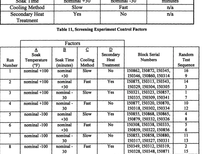
5.6.B Control Factors and Test Plan 63

5.6.C Screening Experiment Procedure 64

5.6.D Screening Experiment Analysis 65

5.6.E Parameter Optimization, Prediction and Confirmation 74

PART 6: MANAGEMENT AND IMPLEMENTATION OF TAGUCHI METHODS IN

THE MANUFACTURING ORGANIZATION 79

6.1 Change in the Manufacturing Organization 79 6.2 Challenges Specific to Corporate Wide Implementation of Taguchi Methods 80 6.3 Implementation of Taguchi Methods on a Project Basis 82

6.3.A The PDCA Structure 82

6.3.B Planning a Taguchi Method Experiment 83 PART 7: SUMMARY, CONCLUSIONS AND RECOMMENDATIONS FOR FUTURE

EFFORTS 87

7.1 Noise Experiment 87

7.2 Screening Experiment 87

7.4 Conclusions

7.5 Recommendations for Future Efforts 90

7.5.A Quantify Components of Variation not Attributable to Test Blocks 90 7.5.B Exploration of Time and Temperature Interaction 90 7.5.C Application of Dynamic Quality Characteristic to the Heat Treating Process 90 Appendix I P-diagram for B-scale Test Block Manufacturing Process 92 Appendix II Noise Experiment Sample Thermocouple Data 93 Appendix III Noise Experiment Hardness Measurement Data 94 Appendix IV L8 (2"~), Resolution IV Orthogonal Array 95

Appendix V Screening Experiment Sample Thermocouple Data 96

Appendix VI Screening Experiment Hardness Measurement Data 98 Appendix VII Screening Experiment Mean and S/N Ratio Table 106

Appendix VIII Error Variance Calculations 107

Appendix IX ANOVA Tables 108

List of Figures

FIGURE 1, MANUFACTURING PROCESS FOR B-SCALE HARDNESS TEST BLOCKS 16

FIGURE 2, GENERIC QUADRATIC LOSS FUNCTION 22

FIGURE 3, DEMONSTRATION OF ROBUSTNESS 25

FIGURE 4, TWO STEP PARAMETER OPTIMIZATION PROCESS 27

FIGURE 5, TYPICAL CONTROL FACTOR TYPES 32

FIGURE 6, MATERIAL PROPERTIES VS. COLD WORK FOR A COPPER ALLOY 39 FIGURE 7, TYPICAL ANNEALING CURVE FOR A COPPER ALLOY: HARDNESS, YIELD STRENGTH

VS. TEMPERATURE 40

FIGURE 8, STEPS IN THE ANNEALING PROCESS FOR A COPPER ALLOY 44 FIGURE 9, INTERACTION BETWEEN TIME AND TEMPERATURE FOR ANNEALING A WROUGHT

COPPER ALLOY ₄₇

FIGURE 10, GENERIC P-DIAGRAM ₅₄

FIGURE 11, HEAT TREATING PROCESS P-DIAGRAM 56

FIGURE 12, NOISE EXPERIMENT ANOM PLOTS 61

FIGURE 13, SCREENING EXPERIMENT FACTOR EFFECT PLOTS 69

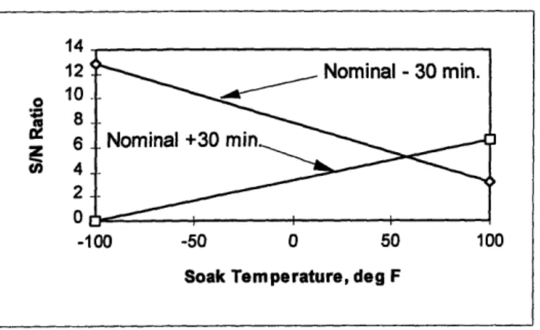
FIGURE 14, SOAK TEMPERATURE/TIME INTERACTION PLOT FOR MEAN HARDNESS 71 FIGURE 15, SOAK TEMPERATURE/TIME INTERACTION PLOT FOR S/N RATIO 74

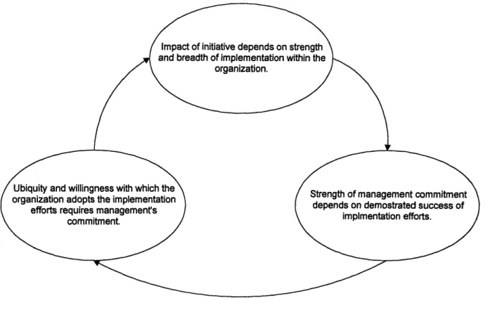
FIGURE 16, MANAGEMENT SUPPORT OF CHANGE IMPLEMENTATION 82

List of Tables

TABLE 1, MACHINING PROCESS NOISE FACTORS 26

TABLE 3, STANDARD TWO-LEVEL L8 ORTHOGONAL ARRAY 33 TABLE 4, B-SCALE TEST BLOCK HARDNESS RANGES AND MATERIALS 37 TABLE 5, TEMPER DESIGNATIONS FOR YELLOW BRASS, UNS 26800 41

TABLE 6, STEPS IN THE ANNEALING PROCESS 44

TABLE 7, SURFACE FINISH CONTROL FACTORS 50

TABLE 8, NOISE FACTOR NAMES AND LEVELS 59

TABLE 9, NOISE EXPERIMENT ORTHOGONAL ARRAY 59

TABLE 10, ANOM SAMPLE CALCULATION 61

TABLE 11, SCREENING EXPERIMENT CONTROL FACTORS 64

TABLE 12, SCREENING EXPERIMENT ORTHOGONAL ARRAY 64

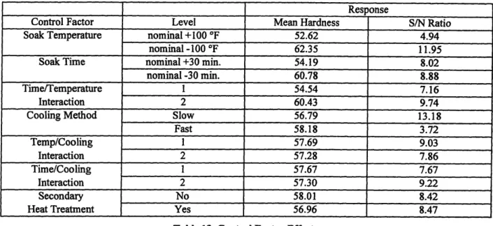
TABLE 13, CONTROL FACTOR EFFECTS 70

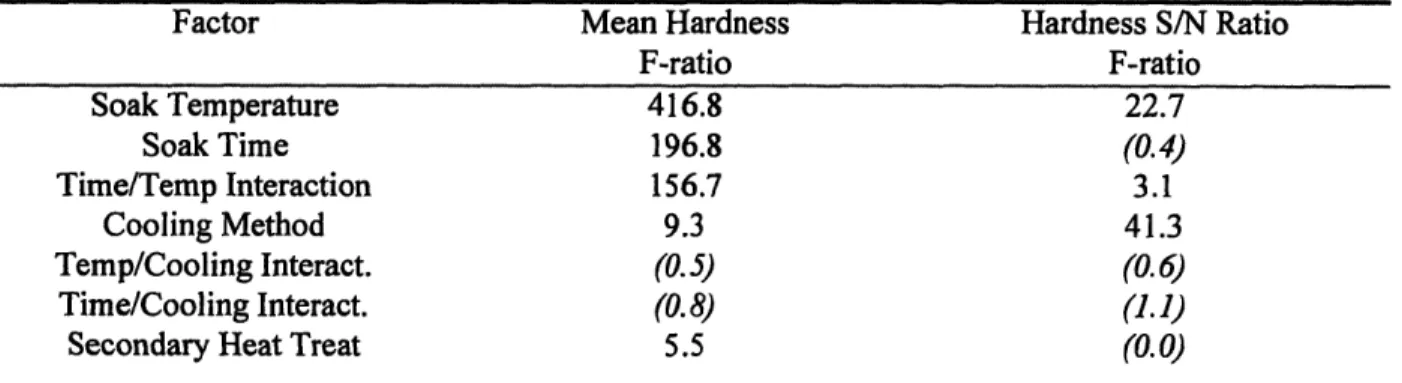
TABLE 14, ANOVA F-RATIOS 73

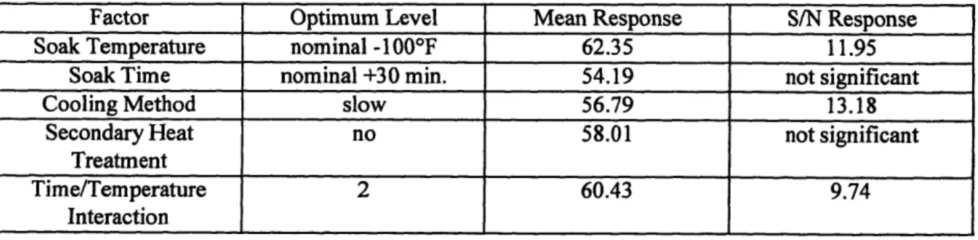
TABLE 15, OPTIMUM FACTOR RESPONSES 75

TABLE 16, MEMBERS OF THE CROSS-FUNCTIONAL TEAM 84

Part

1:

Introduction

1.1

Background

The Wilson Instruments Division of Instron is the leading manufacturer of Rockwell hardness testing equipment and is credited with having established the Rockwell hardness test over 75 years ago. The work contained in this thesis is based on the optimization of a heat treating process used by Wilson Instruments in the manufacture of B-scale standard hardness test blocks. Standard hardness test blocks are used to monitor and calibrate Rockwell

hardness testers during tester commissioning and maintenance programs. They are also used to maintain Wilson Instrument's internal hardness standards.

Wilson Instruments is at the leading edge of Rockwell hardness testing equipment. Most recently, their introduction of the Wilson 2000 series of hardness testers marked a leap ahead of the competition in quality and value. The introduction of the Wilson 2000 series answered the increasing demand of hardness tester users for improved accuracy and repeatability. In support of the customer's demands, Wilson Instruments has also focused considerable efforts on improving the quality of their standard hardness test blocks.

The quality of Wilson's Rockwell C-scale test blocks was improved through the efforts of a Leaders for Manufacturing (LFM) internship completed one year ago. In fact, as a results of those, and previous improvement efforts, the National Institute of Standards and Technology currently purchases, calibrates, and re-sells Rockwell C-scale test blocks

manufactured by Wilson Instruments. The quality of Rockwell B-scale test blocks, which are manufactured from copper alloys, as opposed to steels, however, had not been the subject of quality improvement efforts for several years.

To improve the quality of Rockwell B-scale standard hardness test blocks the Wilson Instruments Division sponsored a second LFM internship. The primary goal of the internship was achieved as the uniformity of the B-scale test blocks was improved by approximately

35%. The enhanced uniformity of the test blocks was achieved by implementing new process control procedures and by improving raw material supplies. Following the primary efforts performed during the LFM internship, an effort to optimize the heat treating process used in the manufacture of B-scale test blocks was performed. The methodology and results of the heat treating process optimization efforts are the subject of this thesis.

1.2

Scope of Thesis

This thesis is limited to the heat treating process used to manufacture B-scale test blocks. It does not discuss the process control procedures or material improvements made over the course of the LFM internship as they are critical to Wilson Instrument's continued leadership in the hardness testing marketplace. Likewise, the exact materials and process parameter settings used in the heat treating process optimization are not provided in the thesis.

1.3

Goals of Thesis

The primary goal of the thesis is to provide the Wilson Instruments Division of Instron with a greater understanding of the B-scale test block heat treating process. A secondary goal is to teach the quality philosophy and quality engineering methods commonly referred to as Taguchi methods to the employees of the Instron Corporation. Instron has an excellent reputation for the quality of their products and, I believe, that their quality efforts could be

further improved through the use of Taguchi methods in their manufacturing process and product development efforts.

Part 2

Background

Rockwell hardness tests are used in research, standardizing, and industrial applications. In all applications there is constant incentive to increase the accuracy and repeatability of hardness testing. In particular, consider the implications of erroneous hardness tests in high-volume manufacturing process control applications. Errors in such applications can be extremely costly and can only be avoided by increasing the quality of the entire hardness testing system.

2.1

Rockwell Hardness Testing System

Hardness is loosely defined as a material's ability to resist deformation. A Rockwell hardness test is a destructive test that determines the hardness of a material by pressing a object of known geometry, called an indentor into the material. For the Rockwell B-scale the indentor is a 1/16" steel sphere. A hardness tester is used to press the indentor into the

material using a sequence of known loads. The hardness tester also records the depth of penetration achieved by the indentor. For the Rockwell B-scale the hardness test sequence is as follows:

I. application of minor load:

A. a 10 kgf load is applied to seat the indentor

B. the start or reference depth of penetration, ystar, is measured II. application of major load:

A. a 100 kgf load is applied to cause an inelastic deformation of the material III. application of minor load:

A. the load is returned to 10 kgf allowing elastic recovery to occur B. the final depth of penetration, y,,an, is measured

The hardness tester records the two depth of penetration measurements and then calculates the material's hardness using the following relationship:

There are many different Rockwell hardness scales which are used to accommodate materials of varying hardness and thickness. The Rockwell scales all use a similar testing method with significant differences arising only in the types of indentors and magnitudes of loads applied.

2.2

Hardness Test Blocks

The primary physical components in the hardness testing system include the hardness tester, indentor, and hardness test block. The hardness test block is used to calibrate hardness testers in commissioning, service, and maintenance applications. In use, the test block is tested using the hardness tester that is undergoing evaluation. If the hardness reading

produced by the hardness tester does not match the known hardness of the test block (within a certain measurement tolerance), the hardness tester is adjusted accordingly.

Each hardness test block is calibrated and stamped with a known hardness by Wilson Instruments. The calibration is performed by measuring the hardness of the test block six times. One of several standardizing hardness testers in the Wilson Instruments Standards Laboratory is used for the calibration measurements. The standardizing testers are monitored and maintained to produce accurate and precise hardness readings. The mean and range of the six readings, and the individual readings themselves, are recorded on a calibration certificate that is shipped with the test block. The mean hardness and a standard measurement tolerance is imprinted on the side of each test block.

The primary problem with B-scale hardness test blocks is that the variation in hardness across the surface of each individual test block is larger than desired. Ideally, the variation in

hardness would be zero. Hardness variation effects both the end user of the test blocks and Wilson Instrument's manufacturing operations. For the end users, be they external customers or Wilson Instruments service people, test block hardness variation can decrease the accuracy of tester calibrations and increase the time required to complete the calibration procedures. For Wilson Instrument's manufacturing operations, test block variation reduces the

manufacturing yield because calibration requirements dictate that any test block with a range

of calibration readings greater than a prescribed value must be discarded. The reduction of test block variation then produces three primary benefits:

1. increased hardness tester calibration accuracy 2. decreased hardness tester calibration efforts 3. increased manufacturing yields

There is an additional benefit to decreasing the variation in hardness test block readings. Since the creation of the Rockwell hardness measurement standard, Wilson Instruments has set the de facto standard for Rockwell hardness. Maintenance of the

standards requires the use of hardness test blocks. The use of more uniform test blocks in the standards maintenance process would create a more stable and easier to maintain standard.

Additionally, two years ago, the National Institute of Standards and Testing (NIST) began issuing standard test blocks for the Rockwell C-scale. Wilson Instruments supplies uncalibrated C-scale test blocks to NIST who then calibrates them using a highly accurate and precise deadweight hardness tester. NIST also plans on issuing standard test blocks for the Rockwell B-scale as well. Wilson Instruments, by improving the uniformity of their B-scale hardness test blocks, could be in a very good position to supply NIST with the uncalibrated test blocks for the national Rockwell B-scale hardness standard.

2.3

Manufacture of

B-Scale Hardness

Test Blocks

B-scale hardness test blocks are produced from a copper alloy using a combination of machining, heat treating, and calibration operations. A block diagram representation of the manufacturing process is given in Figure 1 below. In the figure, the manufacturing steps completed by outside vendors are indicated in italics. Because a substantial portion of the manufacturing process is completed by outside vendors, Wilson Instruments must maintain open and clear channels of information with their vendors. The focus of this thesis is on the heat treating process which is performed by a vendor. A detailed description of the

manufacturing process steps depicted in Figure 1 is not within the scope of the thesis, however; a summary account is presented in the following paragraphs.

Figure 1, Manufacturing Process for B-scale Hardness Test Blocks

The brass mill is responsible for producing the raw material used in the manufacturing process. The raw material must have uniform and stable hardness characteristics which dictate that the material must be uniform in chemical composition and microstructure, and free of chemical impurities and mechanical defects. The brass mill melts the required metallic elements, casts the melt into an ingot, hot-rolls the ingot into sheet, and then anneals and cold rolls the material into a sheet with the desired physical and material characteristics. The brass mill also performs machining processes to the material so that it fits Wilson Instrument's machine tools and so that it has a reasonably smooth surface finish.

The Wilson Instruments Machine Shop is responsible for completing machining operations before and after the heat treating process. Prior to heat treating, the Machine Shop

cuts the copper alloy plate into approximately 2 '/4" diameter blocks(they are referred to as "blocks" as opposed to "discs" because the blocks were originally produced in a rectangular shape), faces the blocks' top and bottom to establish flat and parallel surfaces, chamfers the edges of the blocks, and then stamps each block with a unique serial number. After heat treating, the blocks are returned to the Machine Shop. The Machine Shop removes heat treat scale from the blocks and then laps them to achieve a high level of surface flatness and parallelism. Finally, the block's top surface is polished to a mirror-like finish. Before delivering the test blocks to the Standards Laboratory, the machine shop inspects the test blocks for surface flatness, parallelism, and finish.

The heat treating vendor is responsible for heat treating the test blocks to one of several hardness levels specified by Wilson Instruments. The heat treater places a group of blocks into a gas-fired furnace at a set temperature for a fixed period of time. The blocks are removed from the furnace and allowed to air cool. After the blocks have been allowed to cool several coupon test blocks are tested to determine the mean and variation of hardness on each coupon block's surface. The coupon blocks act as an indicator of the mean and uniformity of hardness achieved by the heat treating process.

The Standards Laboratory is first responsible for inspecting the test blocks for cosmetic flaws. The Standards Laboratory then calibrates the test blocks using standardizing hardness testers. Standardizing hardness testers are specially constructed and maintained to furnish precise and accurate hardness measurements. Each test block is tested for hardness six times. The individual hardness measurements, mean, and range of the six readings are

recorded on a calibration certificate. If the range of hardness on a block is greater than the maximum value specified by a given standardizing body, such as the values provided in ASTM E-18, the test block must be scrapped. After successful calibration the blocks are packaged, placed in finished goods inventory, and, finally, shipped to customers as required.

It should be noted that the uniformity of hardness on a test block is determined

primarily by the Brass Mill and Heat Treater. If the Machine Shop provides smooth, flat, and parallel surfaces, and the Standards Laboratory properly maintains their standardizing testers and test procedures, the remaining sources of variation in hardness are a function of the block's metallurgical condition. The block's metallurgical condition is dependent almost entirely on the processes used by the Brass Mill and Heat Treater. The manufacture of quality hardness test blocks is then very much dependent on the outside vendors used by Wilson Instruments. With a considerable dependence on its vendors it then becomes critical for Wilson Instruments to maintain good relationships with their vendors. Wilson Instruments must simultaneously maintain a knowledge base that allows them to understand their vendor's manufacturing processes as they will dictate the metallurgical condition of the test blocks and thus the test blocks' uniformity of hardness.

It should also be noted that the primary inspection point in the manufacturing process occurs at the very end of the process. Because the inspection does not occur until the blocks reach the Standards Laboratory, a great deal of manufacturing value is lost when a block is scrapped. In addition, because the primary inspection point is at the end of the manufacturing process it becomes difficult to determine the root cause of quality problems. Although inspections may be performed in the manufacturing steps prior to the Standards Laboratory, the accuracy of these tests is difficult to establish primarily due to the fact that the block surfaces are not as smooth, flat, and parallel as they are after the final lapping and polishing operations are performed. Standard material inspection and operating procedures were developed during the LFM internship and their implementation will reduce the risk of introducing quality problems during the manufacturing processes.

Introduction to Taguchi Methods

3.1

History and Current Use of the Taguchi

Method

Taguchi Methods are a system of quality engineering techniques that focus on utilizing engineering knowledge to create the best product or process at the lowest possible cost. Dr. Genichi Taguchi began developing the methods while working to repair Japan's postwar phone system. During the postwar period, the Japanese industries were faced with a shortage of both raw materials and capital and, therefore, were forced to translate their raw materials into useful products as efficiently as possible. Dr. Taguchi combined his knowledge of statistics and engineering into a system that would provide superior outputs while requiring minimal inputs.

Quality methods may be thought to operate in two realms; on-line and off-line. On-line quality methods enhance production output quality by maintaining process control, predicting out-of-control conditions, indicating the root causes of production problems, and measuring production quality. Traditional on-line quality methods include feedback control,

statistical process control, and recording of data. Using on-line quality methods to drive continuous improvements in quality can be costly or downright impossible.

Off-line quality methods can be used to develop or design products and processes with high quality performance characteristics before they are put into full-scale production. Off-line quality activities allow for potentially greater quality improvements because they are less subject to the immediate constraints of production schedules and capital investments.

The quality efforts employed by many U.S. manufacturing firms over the past 50 years have been primarily on-line methods. On-line quality methods control or inspect quality into a product or process whereas off-line quality methods strive to design products or processes

such that they will produce high quality without the need for tightly controlled conditions of customer usage or manufacturing operations.

Taguchi methods are off-line quality methods. They have been widely used by

Japanese manufacturing firms with great success. The methods optimize product and process functional performance by identifying sources of variation and adjusting product and process parameters to suppress the proliferation of variation into a product or process' key functional characteristics. Taguchi's definition of quality may be interpreted as the ability of a product or process to meet its intended performance requirements while being exposed to a broad range of operating conditions. Instead of controlling the operating conditions, Taguchi suggests that the product or process be designed such that changes in operating conditions yield little effect on the intended performance of the product or process.

Taguchi methods have a unique set of basic premises which are not generally included in traditional quality techniques. The Taguchi Method foundations include:

* the costs of quality can be quantified and must include manufacturing costs, life-cycle costs, and losses to society(i.e. environmental impact)

* quality costs are directly related to the variation in functional performance of a product or process

* engineering rather than scientific or statistical methods should be emphasized when completing design and optimization activities

* the effects of uncontrollable variation(noise) on the performance of a product or process should be explicitly included in design and optimization procedures

Through these basic premises, the Taguchi methods provide an engineering approach to product and process design and development that yields high quality systems in a timely manner. Taguchi Methods have achieved wide acceptance by manufacturing companies

worldwide. According to the American Supplier Institute', Taguchi Methods are used primarily to improve existing products and processes. Additional applications which are quickly gaining increased acceptance include new product and process design, flexible technology development, and on-line process control rationalization. The successful use of Taguchi methods in U.S. manufacturing firms to date has been attributed to the fact that the methods:

1. merge the engineering and statistical communities in a useful manner

2. provide a means of quantifying and communicating to management the costs of variability in product or process performance

3. necessarily employ a cross functional team that yields quicker and more effective solutions

4. employ approaches to experimentation that produce results that are more easily interpreted and communicated to others while requiring less time and resources

This thesis is focused on the design of a process and will, therefore, not always refer to both product and process design when speaking generally about the Taguchi methods. Please be aware that the concepts and methods described can be deployed to develop, design, and/or optimize existing and/or new, processes or products.

3.2

The Loss Function

High quality isfreedomfrom costs associated with poor quality. 2

Taguchi's loss function is useful due to its simplicity and its ability to bring together both economic and engineering concepts. The quality loss function establishes the

'American Supplier Institute, World Wide Web Page, http://www.amsup.com/taguchi/, January 12, 1997.

2 Fowlkes, W.Y., Creveling, C.M., Engineering Methods for Robust Product Design -Using Taguchi Methods in Technology and Product Development, Addison-Wesley, Reading, MA, 1995.

approximate loss to manufacturers and consumers due to a deviation in process performance from the intended target. A generic quadratic loss function is shown in Figure 2 below.

Figure 2, Generic Quadratic Loss Function

The standard loss function is a quadratic function that has the following form:

L(y)

=

k(y-m)

L= loss to society, $

k = quality loss coefficient, $ y = actual performance m = target value

Clearly, when the actual performance, y, is equal to the target value, there is no loss. As the deviation from the target increases the loss to society increases by the square of the deviation. Although it may be argued that the shape of the curve is not necessarily quadratic, the parabolic shape has been proven to closely approximate the shape found in situations with substantial sample sizes.

Quadratic Quality Loss Function

49o (A

a

-The quality loss coefficient is determined by the following equation:

k = Ao/(Ao)^2

where:

Ao = 50% customer tolerance limit

Ao = total losses to manufacturer, customer and society at Ao, $

The 50% customer tolerance limit is the point at which 50% of the customers would take some form of economically measurable action due to a product's poor quality. Typical actions might include sending the product back for repair, making a warranty claim, or flat-out refusing to accept the product at the time of delivery. A0, is calculated by summing the

total economic costs incurred at the 50% customer tolerance limit. Ao would then include all material, labor, transportation costs, and other costs due to repair, loss of use, and

replacement.

Taguchi's loss function demonstrates a significant philosophical difference between traditional quality methods in manufacturing firms and the Taguchi method. The traditional method of measuring quality relies on engineering specification limits. Under the traditional methods, quality is improved by producing a greater percentage of output that falls within the specification limits for a given production effort. The loss function, on the other hand, suggests that quality is increased only by reducing deviation from the desired target performance.

Consider the specification limits that are used to accept or reject a ball bearing. The longest bearing life would be realized if the ball bearing were perfectly round. However, to account for the realities of production, an engineering specification limit is set to accept or reject ball bearings based on their roundness. The bearing customer would value a ball bearing that is just barely within the specification limits more or less the same as a bearing that is just barely out of the specification limits. The arbitrary setting of the specification

limits clouds the most important quality issue, that is; the customer derives the most value from a ball bearing that is perfectly round. The loss function demonstrates that there is measurable value to achieving the target performance of perfect roundness, as opposed to just falling within the specification limits.

In a manufacturing firm, the loss function can act as the central means of communicating on-target quality efforts. It is easily communicated throughout an

organization due to its simplicity and graphical nature. The loss function unites the concepts of cost and quality together so that both engineering and management teams can see the benefit of variation reduction efforts. The loss function also supplies its users with a view into the long term costs of quality because it includes both the explicit and implicit costs incurred by the manufacturer, their customers, and the society as a whole.

3.3

Noise and Robustness

The loss function establishes the idea that deviation from intended performance is measurable and costly. Noise and robustness are concepts which may be used to describe a means by which the deviation from intended performance can be reduced. Noise is defined as anything that causes a system's functional characteristic or response to deviate from its

intended target value. Sources of noise are those sources of variation that are either impractical or too costly to control. Robustness is the property a product or process must enjoy if it is to perform at its intended target value in the presence of noise factors. Put another way:

"A product or process is said to be robust when it is insensitive to the effects of sources of variability, even though the sources of variability have not been eliminated. "

The concepts of noise and robustness can be clearly conveyed by modeling a system as a "black box". Consider two systems that are represented in Figure 3 below. Each system

has the same noise inputs. The noise inputs are working to cause variability in each system's output (functional performance or response). The output from system 1 appears to have significantly more variation than system 2. System 2 is more robust that System 1 and we would expect that its quality would be correspondingly higher according to the loss function.

Noise 1 Noise 2 Noise 3

- Input---- -Output

-Noise 1 Noise 2 Noise 3

Figure 3, Demonstration of Robustness

Although there are seemingly endless sources of noise that can effect a system, all noise factors can be categorized into three categories, external, deterioration, and unit-to-unit.

3 Fowlkes, W.Y., Creveling, C.M., Engineering Methods for Robust Product Design -Using Taguchi Methods in Technology and Product Development, Addison-Wesley, Reading, MA, 1995.

25

System 2

External noise factors are sources of variability that come from outside a.process. Deterioration noise factors are sources of variability that occur due to a change within a process. Unit-to-unit noise factors are sources of variability that stem from the inability to produce any two identical items in a production process.

If a simple machining process is considered, the three types of noise factors could be represented as shown in Table 1 below.

Noise Factor Type Machining Process Noise

environmental conditions: as the temperature of the External machine shop changes over the course of the day, the

machine may undergo thermal expansion/contraction wear: as the cutting tool wears the resulting part Deterioration dimensions will change

material: due to differences in the material hardness Unit-to-Unit no two parts will be the same

Table 1, Machining Process Noise Factors

The Taguchi methods use designed experiments and engineering knowledge to determine those noise factors which have an effect on a process. Once the significant noise factors have been identified, further experimentation and engineering is utilized to produce a process design that is robust, that is; the design must be such that it is insensitive to the noise factors which effect the system.

3.4

Parameter Design

Parameter design is used to determine process parameter settings that yield the most robust process at the lowest possible cost. Parameter design considers two types of factors: noise factors and control factors. External, internal, and unit-to-unit noise factors represent the uncontrollable sources of variation that effect the process output. Control factors are those factors which can be controlled at a reasonable cost. The interaction between noise and

control factors is determined using specially designed experiments. By studying the

interaction between the control and noise factors, the control parameter settings that result in the most uniform process output may be identified.

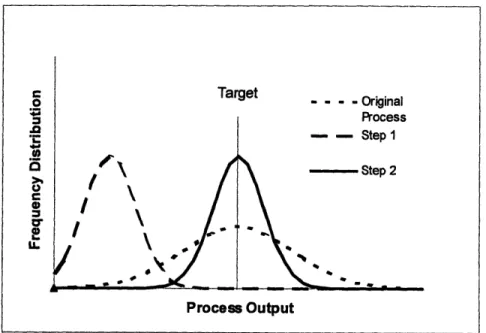
Parameter design is often completed in two steps. First, experiments are used to identify the sources of noise that effect the process most significantly. Second, experiments are completed to gain information about the process control factors. Control factors that have a significant effect on the variability of the process output are set such that the output

variation is minimized. Control factors that effect the mean response of the system but have little effect on the process output variation are called scaling factors. Once the control factors are set to levels that reduce the process output variation, scaling factors may be used to adjust the process output to the desired target. A visual representation of the two step parameter design process is shown in below.

Figure 4, Two Step Parameter Optimization Process

Dr. Taguchi developed a number of tools that make the parameter design method efficient, flexible, and, perhaps most importantly, relatively easy to communicate to those

Target _{- - - - Original} Process - - Step 1 / -, Step 2

I

I

without intimate engineering knowledge. The most widely used tools in parameter design are the quality characteristic, signal-to-noise (S/N) ratio, and orthogonal array. The quality characteristic represents the measured output of a process. The S/N ratio is a measure of robustness that may be specially designed to accommodate many different types of processes and analysis methods. The orthogonal array is a design of experiments array that maximizes the amount of information obtainable from an experiment with an important caveat being that complementary engineering knowledge is available.

3.4.A Quality Characteristic

The quality characteristic is the measured response of a process. Selection of the quality characteristic must be done carefully. Determining how to measure the output from a process may appear to be an artless activity, however, Dr. Taguchi's son cautions users of parameter design in stating:

In parameter design, the most important job of the engineer is to select an effective characteristic to measure as data... We should measure data that relate to the function itself and not the symptoms of

variability... Quality problems take place because of variability in the energy transformations. Considering the energy transformation helps to recognize the function of the system.4

Engineers should not be tempted to measure the quality characteristic in terms of existing quality or accounting metrics. If the metrics chosen for the quality characteristic do not correspond to the process' energy transformation, the engineer will have little success in understanding how the control and noise factors actually effect the process. Measures used for the management of production operations such as yield or defects per unit generally make poor quality characteristics. Measures that relate to the energy transformation such as geometric dimensions, material properties, or temperature provide more useful information about how the control and noise factors effect a process.

4_{Nair, V.N., "Taguchi's Parameter Design: A Panel Discussion." Technometrics 34, 1992.} 28

The quality characteristic must also be selected such that it reduces the chance of measuring interactions between control factors. An interaction between control factors occurs when the effect of one control factor is dependent on another control factor. As will be

discussed in section 3.4.C, Taguchi's parameter design experiments are most effective when interactions between control factors are eliminated through the use of sound engineering judgment. Dr. Taguchi states:

The efficiency of research will drop if it is not possible to find

characteristics that reflect the effects of individual factors regardless of the influence of other factors. 5

Often the quality characteristic can be chosen such that interactions are avoided.

Minimizing the effects of interactions simplifies the experimental and analysis efforts required in a parameter design. By eliminating interactions, the process under consideration becomes easier to understand and control. A process that does not have significant interactions can be engineered for additivity. Additivity in the process means that the effects of each control

factor on the process output is independent of other control factors. Because their are no interactions between the control factors there is no need for multiplicative cross terms when predicting or analyzing the system's response.

Parameter design may be used to optimize a wide array of processes. Accordingly, several different types of quality characteristics have been developed. The types of quality characteristics and examples of their use are shown in Table 2 below.

s Taguchi, G. System of Experimental Design, Vols. I and 2. ASI and Quality Resources 29

Quality Description Examples Characteristic Type

Dynamic Process is optimized speed on an electric mixer over a range of output volume on a stereo amplifier

values temperature in an oven

Nominal-the-best Process is optimized dimension of a part

for one particular mixture of a chemical solution output value electrical resistance of a resistor Smaller-the-better Process is optimized wear of a cutting tool

for an output value that shrinkage in casting

is as near to zero as power loss through a powertrain possible

Larger-the-better Process is optimized efficiency of a furnace for an output value that strength of a structure is as large as possible fatigue resistance of a weld

Table 2, Types of Quality Characteristics

Dr. Taguchi believes that the most powerful type of characteristic is the dynamic type. He has been quoted as saying "the adoption and continued utilization of the dynamic

approach represents the path that virtually all world-class organizations will take to establish themselves as leaders in their industries."6 The dynamic characteristic can be applied to processes where the output of the system changes as the input to the system is adjusted. The dynamic method optimizes a process over a range of expected outputs, whereas the other quality characteristics optimize the process at a fixed output level only.

3.4.B Signal-to-Noise (S/N) Ratio

The S/N ratio is used to measure the robustness of a process. The "signal"

(numerator) represents the response of the process as measured by the quality characteristic. The "noise" (denominator) represents the magnitude of the uncontrollable sources of

variability in the process. The S/N ratio is calculated in a different manner for each type of quality characteristic. However, regardless of the type of process being studied, when the S/N

ratio is maximized, the robustness of the process is also maximized. A custom S/N ratio can be developed for unique processes, however all S/N ratios should:

1. measure the process output variability that is caused by noise factors 2. be independent of shifting the mean response of the process to its target 3. be a relative measure so that it can be used for comparative purposes 4. reduce the potential for interactions between control factors

One of the most common S/N ratios is the static, nominal-the-best type. In the nominal-the-best case the process is optimized for a known target response value. For the static, nominal-the-best quality characteristic, the S/N ratio is defined as:

2

S / N = 10 log _where: y = mean process output and s2 = process output variance

--2

It can be seen that an increase in the signal, y2 _{or a decrease in the noise, s}2 _causes the S/N ratio to increase. Intuitively, this makes sense as an increase in "signal" or a decrease in "noise" should be considered a move in the right direction for the process if it is to be made more robust. Also note that the equation does not contain the target value; this is because the S/N ratio is independent of shifting the mean response of the process to the target value.

The base 10 log function puts the S/N ratio into decibel units. The log transformation is accepted as standard Taguchi method procedure and grew out of Dr. Taguchi's work in the communications industry. However, use of the log function is more than just a relic because it "makes the metric more additive in the statistical sense."2 _{To see why the log function} promotes additivity one needs only to look at one of the log function's basic properties, that is, log(A x B) = log A + Log B. Given two control factors, A and B, and an interaction

6 _{Wilkens, J., "Introduction to Quality Engineering and Robust Design." American Supplier Institute, 10th}

between the two, A x B, then the log of the response, log (A x B), becomes additive in that it may be treated as log A + log B.

The S/N ratio is frequently plotted together with the mean response of the process to demonstrate the effects of an individual control factor. Figure 5 shows two combinations of S/N ratio and mean response that could be encountered while analyzing a parameter design experiment. The top two plots represent the mean response and S/N ratio of a control factor that could be used as a scaling factor. Note that in the top plots the mean process output can be shifted (presumably to the desired target value) without causing a decrease in the S/N ratio and, hence, process robustness is maintained. The bottom plots demonstrate a control factor that should be set at its higher level in order to increase process robustness. In the bottom plots there would be serious loss of process robustness if the control factors low setpoint were used.

Scaling Factor

Mean _SIN

Low High Low High

Factor Set to Maximize Robustness

Mean SIN

Low High Low High

(setpoint) (setpoint)

Figure 5, Typical Control Factor Types

There are numerous possible combinations of mean response and S/N ratio. A control factor that has little effect on either mean response or the S/N ratio may be adjusted to the most economical level. In order to locate those control factors that are useful for shifting the mean response to the target and increasing robustness, it is common to include as many control factors in the parameter design process as is practical.

3.4.C Orthogonal Arrays

To reduce the experimentation effort required in his parameter design work, Dr. Taguchi adopted the use of orthogonal arrays. Orthogonal arrays are designed experiment arrays that have the property of orthogonality; that is, the factors in the array are balanced and statistically independent. The basic terminology used to indicate an orthogonal array is Lx, where L indicates that array is orthogonal and x dictates the number of individual experiments in the array. An example of and L8array is shown in Table 3 below.

2 1 1 2 2 4 1 2 1 2 6 7 1 1 2 2 2 2 1 1 S21 2 1 2 1 2 6 2 1 2 2 1 2 1 7 2 2 1 1 2 2 1 8 2 2 1 2 1 1 2

Table 3, Standard Two-Level L8 Orthogonal Array

In many Taguchi applications the orthogonal array is used in an inner and outer array configuration. The inner array generally contains the control factors while the outer array contains the noise factors. The inner array provides information regarding the effects of control parameters and generates the "signal" in the S/N ratio. The outer array acts to stress the system giving the necessary "noise" in the S/N ratio.

The total experimental effort can be considerable when both inner and outer arrays are of significant size. For example, if an experiment were to use and L, inner array and a L8

Run 1

2

3

outer array, the total effort would require 64 experiments. Each of the control factor settings dictated by the inner array would have to be repeated for each of the eight noise factor settings required for the outer array. To reduce the experimental effort, the noise array can be

minimized by confounding or combining the noise factors. Preliminary experiments are used to provide the information necessary for confounding the noise factors and the resulting outer array becomes an L2. By confounding the noise factors the total test effort becomes sixteen noise and sixteen main experiments for a factor of two savings. Confounding can not always be used; however, in most parameter design efforts it is extremely useful for reducing the experimental efforts required.

For parameter design the orthogonal array is preferred to other experimental arrays because it provides a great deal of useful information while using the least possible number of experiments. An orthogonal array that can test the effects of seven parameters is shown in Table 3. Testing of seven parameters with a traditional full-factorial experiment would require 128 experiments, an order-of-magnitude greater effort.

Although the orthogonal arrays decrease the experimentation resources required for parameter design, the real benefit offered by orthogonal arrays is their balance. Balance in the array can be seen by noting that within every column each factor level is used the same

number of times. Balance between the factors is also evident by noting that for a given factor held at one level, each and every other factor occurs at its two respective levels the same number of times. For example, when factor 1 is held at level 1, factor 3 has the pattern 1, 1, 2, 2, while factor 5 has the pattern 1, 2, 1, 2, (see Table 3 above). Each of the factor levels occur twice although there are differences in pattern.

Balance, or orthogonality, in the array isolates the effects of individual parameters making them easier to analyze and control. For example, when a factor level is found to produce a change in the process output, be it measured as the mean response or S/N ratio, the

change can be directly attributed to that factor alone and not the other factors. The effects of the other factors need not be accounted for because each of the other factors occur an equal number of times at both their levels and; therefore, their factor level effects cancel one another out.

The weakness of orthogonal arrays is that they cannot be used if the experimenter does not have a good understanding of the process under consideration. Traditional experimental

design arrays are powerful in that they are able to quantify interactions in a process. If interactions are present and not accounted for in an orthogonal experiment, the array will produce useless or misleading information. Generally speaking, interactions are avoided in parameter design; however, if they are unavoidable, modified orthogonal arrays may be used to accommodate them.

One final benefit that is frequently noted about the orthogonal array is that they are relatively easy to manipulate. Traditional experimental design arrays can be difficult to work with for engineers who do not have rigorous statistical backgrounds. Because the orthogonal arrays are more easily applied, the parameter design engineers can presumably spend more time on engineering and experimentation than on manipulation and analysis of the

experimental arrays. The combined simplicity of the orthogonal array and the emphasis on eliminating interactions makes the output of the orthogonal array more easily communicated throughout a cross-functional organization.

The information presented in the last few sections of this paper contains a recurring theme; that is, engineering knowledge is necessary to employ Taguchi methods successfully. In fact, Dr. Taguchi has recommended that 80% of a parameter design team's efforts be spent before any experiments are actually completed. A failure to plan for interactions is cited as being the largest cause of failure in use of the Taguchi Method experiments. In following with Dr. Taguchi's advice, a search of available information on related heat treating processes

and Taguchi method applications was completed. The results of this search are the subject for the following section of this thesis.

Part 4:

Engineering Knowledge of Related Heat Treating

Processes and Taguchi Method Applications

Before the Taguchi methods are applied to the hardness test block heat treating process, a study of related heat treating and Taguchi methods applications is necessary. A review of the available literature will provide information that would otherwise have to be re-learned through costly experimentation.

4.1

Purpose of Heat Treating Hardness Test Blocks

The purpose of heat treating B-scale hardness test blocks is to reduce the test block's hardness. By using the heat treating process Wilson Instruments is not required to hold raw material inventory for all the hardness ranges they produce (see Table 4). It is possible to use brass plate with a hardness of HRB 80 or greater for all the B-scale test blocks offered by Wilson except for the HRB 95 test block. The HRB 95 test block is produced from steel.

Nominal Hardness Hardness Range Material

(HRB) (HRB)

0 Below 5.0 Copper alloy

10 5.0- 14.9 __ 20 15.0-24.9 __ 30 25.0- 34.9 __ 40 35.0-44.9

II

II

II

II

Table 4, B-Scale Test Block Hardness Ranges and Materials

The heat treating process used by Wilson Instruments is called annealing. In general, annealing refers to any heat treating process wherein a metal is brought to an elevated

conditions in order to reduce hardness. The annealing process used for test blocks is called a partial annealing process. The partial annealing process must be controlled to yield two important results, they are:

1. on-target average hardness of the test blocks 2. high uniformity of hardness on each test block

As will be discussed in the following section, a partial anneal is difficult to control. The changes which occur in the metal's structure during a partial anneal are both

heterogeneous and rapid. In addition to being difficult to control, there is very little information published on partial annealing. In fact, the published literature advises that partial annealing be avoided in commercial applications.

4.2

Commercial Annealing Processes

4.2.A Purpose of Commercial Heat Treating Processes

Commercial annealing processes are performed on metals to facilitate subsequent cold working, improve mechanical, electrical or thermal properties, enhance machinibility, and/or stabilize part dimensions. Annealing processes are used for both ferrous and non-ferrous metals; however, only non-ferrous annealing processes will be discussed in this document. To further limit the discussion of annealing processes, only those metal products and processes which are closely similar to those used in the manufacture of B-scale test blocks will be considered. That is, the information will be focused on annealing processes that are used in the manufacture of wrought copper alloy products.

4.2.B Brass Strip: An example of Cold Work and Annealing

In the manufacture of wrought copper alloy products the annealing process is used primarily to facilitate cold-working processes. As an example, consider the production of

0.04 in. brass strip. The metal may begin the cold rolling process at some thickness which is considerably greater than the final thickness, say 0.40" thick. When the material is cold rolled both its strength and hardness increase as is indicated in Figure 6. These properties increase

because the strain placed into the material increases the density of dislocations in the

material's metallic structure. The dislocations act as barriers to further strain in the material and thereby increase both its strength and hardness.

Material Properties vs. Cold Work

I uuu 900 I. 800 700 600 c 500 400 Co 300 200 100 0 Izu 100 80o 60 i 40 E 20 0 0 10 20 30 40 50 60 70 Reduction in Thickness, %

Figure 6, Material Properties vs. Cold Work for a Copper Alloy

When the strength and hardness of the metal increases it becomes more costly to deform the metal. In addition, the metal may become brittle with high levels of cold work, potentially leading to fracture and a stalled production line. To reduce the strength and hardness of the heavily cold-worked metal strip it is subjected to an annealing process. A typical non-ferrous alloy's properties will change during the annealing process according to the curves shown in Figure 7 below.

Annealing Curve, 1 Hour Soak Time IloA nn 90 80 Im_{S 70} : 60 v 50₅₀ E 40 3 30 S 20 10 0 700 600 500 j 400 C 300 E 200 100 0 0 100 200 300 400 500 600 700 Temperature, deg C

Figure 7, Typical Annealing Curve for a Copper Alloy: Hardness, Yield Strength vs. Temperature

In a step-wise manner the rolling and annealing functions are performed until the strip is reduced to a thickness that is close to its final desired thickness. For continuous products, such as strip, wire, and sheet, annealing is frequently done in a continuous process where the metal is passed through a annealing furnace. The temperature of the furnace and the speed at which the material passes through the furnace are controlled to produce the desired results. Other products, such as slabs, plates, and heavy sections are batch annealed. To produce the desired results in batch annealing the furnace temperature, soak time, and furnace load must be controlled. The inter-process anneals are controlled to yield the desired material properties at the lowest possible manufacturing cost.

4.2.C Full vs. Partial Annealing

Wrought copper alloys are produced at numerous tempers. The product's temper designates its material properties and is set according to American Society for Testing and Materials (ASTM) specifications. For example, yellow brass (UNS No. 26800), is produced according to ASTM B36/B36M with the temper designations and material property

requirements as shown in Table 5 below.

Temper Designation Tensile Strength, MPa Rockwell Hardness, HRB, for > 0.036" thick M20 As hot-rolled 275-345 N/A HO1 Quarter-hard 340-405 44-65 H02 Half-hard 380-450 60-74 H03 Three-quarter hard 425-495 73-80 H04 Hard 470-540 78-84 H06 Extra-hard 545-615 85-89 H08 Spring 595-655 89-92 H 10 Extra Spring 620-685 90-93

Table 5, Temper Designations for Yellow Brass, UNS 268007

A product's temper is generally determined by final processing steps that add cold work to the material. The tempers are determined by cold working, as opposed to annealing, for two reasons:

1. it requires less energy and fewer process steps to cold work the material to its final dimensions and material properties

2. it is relatively difficult to control the material properties resulting from an annealing process

When an annealing process is used to produce a product with specific material properties, the annealing process is called partial annealing or annealing to temper.

Commercial heat treaters generally avoid these processes as the resulting on-target success rates are quite poor. In fact, and American Society of Metals publication states, "It is impracticable to anneal for definite properties of tensile strength or hardness between the normal cold worked and fully recrystallized or softened range because of the extremely rapid change of properties with only a small change in metal temperature."'

7 American Society for Testing and Materials, Designation B 36/ B 36M, Standard Specification for Brass Plate,

Sheet, Strip, and Rolled Bar, 1995.

8 American Society for Metals, Source Book on Copper and Copper Alloys, Section VIII: Heat Treating, Metals Park, OH, 1979.

There are several variables which effect the outcome of the annealing process including, but not limited to:

I. furnace temperature

2. time the product spends in the furnace 3. degree of cold-work in the material 4. furnace load(utilization)

5. product dimensions

6. material chemical composition

To avoid the cost of controlling the above variables, the common practice is to use full anneal processes. A full anneal brings the material to its minimum strength and hardness. In Figure 7, a full anneal would correspond to the portion of the curve above approximately 500 *C. In this region of the annealing curve the material properties are less sensitive to variations in the time and temperature process parameters. In full annealing the material approaches a state of equilibrium. When a partial anneal is performed the dynamics of the process are much faster than when a full anneal is used. Consequently, the material properties are highly sensitive to the variables listed above and considerable efforts must be made to control the process variables in order to produce consistent on-target results. The next section will discuss technical information regarding the annealing process.

4.3

Annealing: Technical Details

To this day, the mechanics of annealing processes are not fully understood. The available literature on the subject is difficult to use for one of the following two reasons:

1. the information relies on experimental data that is strictly context dependent 2. the information is in the form of theoretical dissertations that are complex and

The most informative annealing references located by the author are a recently published monograph', compiled by Mr. John Humphreys and Mr. Max Hatherly, and The American Society of Materials(ASM) Handbooks, Volumes 2'0 and 4". A summary of

information applicable to the heat treating of copper alloys will be presented in this section. At this point, however, it is worth quoting the preface of the Humphrey and Hatherly monograph:

It is not easy to write a book on recrystallization, because although it is a clearly defined subject, many aspects are not well understood and the experimental evidence is often poor and conflicting. It would have been desirable to quantify all aspects of the phenomena and to derive the theories from first principles. However, this is not yet possible, and the reader will find within this book a mixture of relatively sound theory, reasonable assumptions and conjecture. There are two main reasons for our lack of progress. First, we cannot expect to understand recovery and recrystallization in depth unless we understand the nature of the deformed state which is the precursor, and that is still a distant goal. Second, although some annealing processes, such as recovery and grain growth are reasonably homogenous, others, such as recrystallization and abnormal grain growth are heterogeneous, relying on local instabilities and evoking parallels with apparently chaotic events such as weather.

(emphasis by the author)

The published technical information, albeit sparse, provides a useful basis for the experimental efforts presented in later sections of this thesis.

4.3.B Steps in the Annealing Process

There are a number of process steps that occur during the annealing process. The steps are described in Table 6 and their positions on a typical annealing curve are illustrated in Figure 8.

9 Humphreys, F. J., Hatherly, M., Recrystallization and Related Annealing Phenomena, Pergamon, Elsevier Science Ltd., Tarrytown, NY, 1995.

'o ASM Handbook, Formerly Tenth Edition, Metals Handbook, Volume 2, Properties and Selection: Nonferrous

Alloys and Special-Purpose Materials, ASM International, 1995.