Artificial Neurogenesis: An Introduction and Selective Review

HAL Id: hal-01351738

https://hal.archives-ouvertes.fr/hal-01351738

Submitted on 5 Aug 2016

HAL is a multi-disciplinary open access

archive for the deposit and dissemination of

sci-entific research documents, whether they are

pub-lished or not. The documents may come from

teaching and research institutions in France or

abroad, or from public or private research centers.

L’archive ouverte pluridisciplinaire HAL, est

destinée au dépôt et à la diffusion de documents

scientifiques de niveau recherche, publiés ou non,

émanant des établissements d’enseignement et de

recherche français ou étrangers, des laboratoires

publics ou privés.

Distributed under a Creative Commons Attribution| 4.0 International License

Artificial Neurogenesis: An Introduction and Selective

Review

Taras Kowaliw, Nicolas Bredeche, Sylvain Chevallier, René Doursat

To cite this version:

Taras Kowaliw, Nicolas Bredeche, Sylvain Chevallier, René Doursat. Artificial Neurogenesis: An

In-troduction and Selective Review. Springer; Taras Kowaliw, Nicolas Bredeche, René Doursat. Growing

Adaptive Machines, 557, pp.1-60, 2014, Studies in Computational Intelligence, 978-3-642-55336-3.

�10.1007/978-3-642-55337-0_1�. �hal-01351738�

Artificial Neurogenesis: An Introduction

and Selective Review

Taras Kowaliw, Nicolas Bredeche, Sylvain Chevallier and René Doursat

Abstract In this introduction and review—like in the book which follows—we

explore the hypothesis that adaptive growth is a means of producing brain-like machines. The emulation of neural development can incorporate desirable character-istics of natural neural systems into engineered designs. The introduction begins with a review of neural development and neural models. Next, artificial development— the use of a developmentally-inspired stage in engineering design—is introduced. Several strategies for performing this “meta-design” for artificial neural systems are reviewed. This work is divided into three main categories: bio-inspired representa-tions; developmental systems; and epigenetic simulations. Several specific network biases and their benefits to neural network design are identified in these contexts. In particular, several recent studies show a strong synergy, sometimes interchange-ability, between developmental and epigenetic processes—a topic that has remained largely under-explored in the literature.

T. Kowaliw (

B

Institut des Systèmes Complexes - Paris Île-de-France, CNRS, Paris, France e-mail: taras@kowaliw.ca

N. Bredeche

Sorbonne Universités, UPMC University Paris 06, UMR 7222 ISIR,F-75005 Paris, France

e-mail: nicolas.bredeche@upmc.fr N. Bredeche

CNRS, UMR 7222 ISIR,F-75005 Paris, France S. Chevallier

Versailles Systems Engineering Laboratory (LISV), University of Versailles, Velizy, France

e-mail: sylvain.chevallier@uvsq.fr R. Doursat

School of Biomedical Engineering, Drexel University, Philadelphia, USA e-mail: rene.doursat@drexel.edu

T. Kowaliw et al. (eds.), Growing Adaptive Machines, 1

Studies in Computational Intelligence 557, DOI: 10.1007/978-3-642-55337-0_1, © Springer-Verlag Berlin Heidelberg 2014

This book is about growing adaptive machines. By this, we mean producing programs that generate neural networks, which, in turn, are capable of learning. We think this is possible because nature routinely does so. And despite the fact that animals—those multicellular organisms that possess a nervous system—are stagger-ingly complex, they develop from a relatively small set of instructions. Accordstagger-ingly, our strategy concerns the simulation of biological development as a means of

gener-ating, in contrast to directly designing, machines that can learn. By creating

abstrac-tions of the growth process, we can explore their contribution to neural networks from the viewpoint of complex systems, which self-organize from relatively simple agents, and identify model choices that will help us generate functional and useful artefacts. This pursuit is highly interdisciplinary: it is inspired by, and overlaps with, computational neuroscience, systems biology, machine learning, complex systems science, and artificial life.

Through growing adaptive machines, our ambition is also to contribute to a radical reconception of engineering. We want to focus on the design of component-level behaviour from which higher-level intelligent machines can emerge. The success of this “meta-design” [63] endeavour will be measured by our capacity to generate new learning machines: machines that scale, machines that adapt to novel environments, in short, machines that exhibit the richness we encounter in animals, but presently eludes artificial systems.

This chapter and the book that it introduces are centred around developmental and learning neural networks. It is a timely topic considering the recent resurgence of the neural paradigm as a major representation formalism in many technological areas, such as computer vision, signal processing, and robotic controllers, together with rapid progress in the modelling and applications of complex systems and highly decentralized processes. Researchers generally establish a distinction between

struc-turaldesign, focusing on the network topology, and synaptic design, defining the

weights of the connections in a network [278]. This book examines how one could create a biologically inspired network structure capable of synaptic training, and blend synaptic and structural processes to let functionally suitable networks self-organize. In so doing, the aim is to recreate some of the natural phenomena that have inspired this approach.

The present chapter is organized as follows: it begins with a broad description of neural systems and an overview of existing models in computational neuroscience. This is followed by a discussion of artificial development and artificial neurogenesis in general terms, with the objective of presenting an introduction and motivation for both. Finally, three high-level strategies related to artificial neurogenesis are explored: first, bio-inspired representations, where network organization is inspired by empirical studies and used as a template for network design; then, developmental

simulation, where networks grow by a process simulating biological embryogenesis;

finally, epigenetic simulation, where learning is used as the main step in the design of the network. The contributions gathered in this book are written by experts in the field and contain state-of-the-art descriptions of these domains, including reviews of original research. We summarize their work here and place it in the context of the meta-design of developmental learning machines.

1 The Brain and Its Models

1.1 Generating a Brain

Natural reproduction is, to date, the only one known way to generate true “intelli-gence”. In humans, a mere six million (6 × 106_{) base pairs, of which the majority}

is not directly expressed, code for an organism of some hundred trillion (1014_{) cells.}

Assuming that a great part of this genetic information concerns neural development and function [253], it gives us a rough estimate of a brain-to-genome “compression ratio”. In the central nervous system of adult humans, which contains approximately 8.5×1010neural cells and an equivalent number of non-neural (mostly glial) cells [8], this ratio would be of the order of 104. However, the mind is not equal to its neurons, but considered to emerge from the specific synaptic connections and transmission efficacies between neurons [234,255]. Since a neural cell makes contacts with 103

other cells on average,1_{the number of connections in the brain reaches 10}14_{, raising}

our compression ratio to 108_{, a level beyond any of today’s compression algorithms.}

From there, one is tempted to infer that the brain is not as complex as it appears based solely on the number of its components, and even that something similar might be generated via a relatively simple parallel process. The brain’s remarkable structural complexity is the result of several dynamical processes that have emerged over the course of evolution and are often categorized on four levels, based on their time scale and the mechanisms involved:

level time scale change

phylogenic generations genetic: randomly mutated genes propagate or perish with the success of their organisms

ontogenic days to years cellular: cells follow their genetic instructions, which make them divide, differentiate, or die

epigenetic seconds to days cellular, connective: cells respond to external stimuli, and behave differently depending on the environment; in neurons, these changes include contact modifica-tions and cell death

inferential milliseconds to seconds connective, activation: neurons send electrical signals to their neighbours, generating reactions to stimuli

However, a strict separation between these levels is difficult in neural development and learning processes.2_{Any attempt to estimate the phenotype-to-genotype}

com-1_{Further complicating this picture are recent results showing that these connections might}

them-selves be information processing units, which would increase this estimation by several orders of magnitude [196].

2_{By epigenetic, we mean here any heritable and non-genetic changes in cellular expression. (The}

same term is also used in another context to refer strictly to DNA methylation and transcription-level mechanisms.) This includes processes such as learning for an animal, or growing toward a light source for a plant. The mentioned time scale represents a rough average over cellular responses to environmental stimuli.

pression ratio must also take into account epigenetic, not just genetic, information. More realistic or bio-inspired models of brain development will need to include models of environmental influences as well.

1.2 Neural Development

We briefly describe in this section the development of the human brain, noting that the general pattern is similar in most mammals, despite the fact that size and durations vastly differ. A few weeks after conception, a sheet of cells is formed along the dorsal side of the embryo. This neural plate is the source of all neural and glial cells in the future body. Later, this sheet closes and creates a neural tube whose anterior part develops into the brain, while the posterior part produces the spinal cord. Three bulges appear in the anterior part, eventually becoming the forebrain, midbrain, and hindbrain. A neural crest also forms on both sides of the neural tube, giving rise to the nervous cells outside of the brain, including the spinal cord. After approximately eight weeks, all these structures can be identified: for the next 13-months they grow in size at a fantastic rate, sometimes generating as many as 500,000 neurons per minute.

Between three to six months after birth, the number of neurons in a human reaches a peak. Nearly all of the neural cells used throughout the lifetime of the individual have been produced [69,93]. Concurrently, they disappear at a rapid rate in various regions of the brain as programmed cell death (apoptosis) sets in. This overproduction of cells is thought to have evolved as a competitive strategy for the establishment of efficient connectivity in axonal outgrowth [34]. It is also regional: for instance, neural death comes later and is less significant in the cortex compared to the spinal cord, which loses a majority of its neurons before birth.

Despite this continual loss of neurons, the total brain mass keeps increasing rapidly until the age of three in humans, then more slowly until about 20. This second peak marks a reversal of the trend, as the brain now undergoes a gradual but steady loss of matter [53]. The primary cause of weight increase can be found in the connective structures: as the size of the neurons increase, so does their dendritic tree and glial support. Most dendritic growth is postnatal, but is not simply about adding more connections: the number of synapses across the whole brain also peaks at eight months of age. Rather, mass is added in a more selective manner through specific phases of neural, dendritic, and glial development.

These phenomena of maturation—neural, dendritic, and glial growth, combined with programmed cell death—do not occur uniformly across the brain, but regionally. This can be measured by the level of myelination, the insulation provided by glial cells that wrap themselves around the axons and greatly improve the propagation of membrane potential. Taken as an indication of more permanent connectivity, myelination reveals that maturation proceeds in the posterior-anterior direction: the

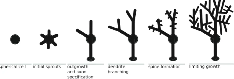
Fig. 1 Illustration of the general steps in neural dendritic development

spinal cord and brain stem (controlling vital bodily function) are generally mature at birth, the cerebellum and midbrain mature in the few months following birth, and after a couple of years the various parts of the forebrain also begin to mature. The first areas to be completed concern sensory processing, and the last ones are the higher-level “association areas” in the frontal cortex, which are the site of myelination and drastic reorganization until as late as 18-years old [69]. In fact, development in mammals never ends: dendritic growth, myelination, and selective cell death continue throughout the life of an individual, albeit at a reduced pace.

1.2.1 Neuronal Morphology

Neurons come in many types and shapes. The particular geometric configuration of a neural cell affects the connectivity patterns that it creates in a given brain region, including the density of synaptic contacts with other neurons and the direction of sig-nal propagation. The shape of a neuron is determined by the outgrowth of neurites, an adaptive process steered by a combination of genetic instructions and environmental cues.

Although neurons can differ greatly, there are general steps in dendritic and axonal development that are common to many species. Initially, a neuron begins its life as a roughly spherical body. From there, neurites start sprouting, guided by growth cones. Elongation works by addition of material to relatively stable spines. Sprouts extend or retract, and one of them ultimately self-identifies as the cell’s axon. Dendrites then continue to grow out, either from branching or from new dendritic spines that seem to pop up randomly along the membrane. Neurites stop developing, for example, when they have encountered a neighbouring cell or have reached a certain size. These general steps are illustrated in Fig.1[230,251].

Dendritic growth is guided by several principles, generally thought to be controlled regionally: a cell’s dendrites do not connect to other specific cells but, instead, are drawn to regions of the developing brain defined by diffusive signals. Axonal growth

tends to be more nuanced: some axons grow to a fixed distance in the direction of a simple gradient; others grow to long distances in a multistage process requiring a large number of guidance cells. While dendritic and axonal development is most active during early development, by no means does it end at maturity. The continual generation of dendritic spines plays a crucial role throughout the lifetime of an organism.

Experiments show that neurons isolated in cultures will regenerate neurites. It is also well known that various extracellular molecules can promote, inhibit, or other-wise bias neurite growth. In fact, there is evidence that in some cases context alone can be sufficient to trigger differentiation into specific neural types. For example, the introduction of catalysts can radically alter certain neuron morphologies to the point that they transform into other morphologies [230]. This has important consequences on any attempt to classify and model neural types [268].

In any case, the product of neural growth is a network possessing several key properties that are thought to be conducive to learning. It is an open question in neuroscience how much of neural organization is a result of genetic and epigenetic targeting, and how much is pure randomness. However, it is known that on the meso-scopic scale, seemingly random networks have consistent properties that are thought to be typical of effective networks. For instance, in several species, cortical axonal outgrowth can be modelled by a gamma distribution. Moreover, cortical structures in several species have properties such as relatively high clustering along certain axes, but not other axes [28, 146]. Cortical connectivity patterns are also “small-world” networks (with high local specialization, and minimal wiring lengths), which pro-vide efficient long-range connections [263] and are probably a consequence of dense packing constraints inside a small space.

1.2.2 Neural Plasticity

There are also many forms of plasticity in a nervous system. While neural cell behaviour is clearly different during development and maturity (for instance, the drastic changes in programmed cell death), many of the same mechanisms are at play throughout the lifetime of the brain. The remaining differences between devel-opmental and mature plasticity seem to be regulated by a variety of signals, especially in the extracellular matrix, which trigger the end of sensitive periods and a decrease in spine formation dynamics [230].

Originally, it was Hebb who postulated in 1949 what is now called Hebbian

learn-ing: repeated simultaneous activity (understood as mean-rate firing) between two

neurons or assemblies of neurons reinforces the connections between them, further encouraging this co-activity. Since then, biologists have discovered a great variety of mechanisms governing synaptic plasticity in the brain, clearly establishing recipro-cal causal relations between wiring patterns and firing patterns. For example, long-term potentiation (LTP) and long-long-term depression (LTD) refer to ositiveor negative

changes in the probability of successful signal transmission from a resynapticaction potential to the generation of a postsynaptic potential. These “long-term” changes can last for several minutes, but are generally less pronounced over hours or days [230]. Prior to synaptic efficacies, synaptogenesis itself can also be driven by activity-dependent mechanisms, as dendrites “seek out” appropriate partner axons in a process that can take as little as a few hours [310]. Other types of plasticity come from glial cells, which stabilize and accelerate the propagation of signals along mature axons (through myelination and extracellular regulation), and can also depend on activity [135].

Many others forms and functions of plasticity are known, or assumed, to exist. For instance, “fast synaptic plasticity”, a type of versatile Hebbian learning on the 1-ms time scale, was posited by von der Malsburg [286–288]. Together with a neural code based on temporal correlations between units rather than individual firing rates, it provides a theoretical framework to solve the well-known “binding problem”, the question of how the brain is able to compose sensory information into multi-feature concepts without losing relational information. In collaboration with Bienenstock and Doursat, this assumption led to a format of representation using graphs, and models of pattern recognition based on graph matching [19–21]. Similarly, “spike-timing dependent plasticity” (STDP) describes the dependence of transmission efficacies between connected neurons on the ordering of neural spikes. Among other effects, this allows for pre-synaptic spikes which precede post-synaptic spikes to have greater influence on the resulting efficacy of the connection, potentially capturing a notion of causality [183]. It is posited that Hebbian-like mechanisms also operate on non-neural cells or neural groups [310]. “Metaplasticity” refers to the ability of neurons to alter the threshold at which LTP and LTD occur [2]. “Homeostatic plas-ticity” refers to the phenomenon where groups of neurons self-normalize their own level of activity [208].

1.2.3 Theories of Neural Organization

Empirical insights into mammalian brain development have spawned several theories regarding neural organization. We briefly present three of them in this section:

nativism, selectivism, and neural constructivism.

The nativist view of neural development posits a strong genetic role in the construction of cognitive function. It claims that, after millions of years of evo-lutionary shaping, development is capable of generating highly specialized, innate neural structures that are appropriate for the various cognitive tasks that humans accomplish. On top of these fundamental neural structures, details can be adjusted by learning, like parameters. In cognitive science, it is argued that since children learn from a relative poverty of data (based on single examples and “one-shot learning”), there must be a native processing unit in the brain that preexists independently of environmental influence. Famously, this hypothesis led to the idea of a “universal grammar” for language [36], and some authors even posit that all basic concepts are innate [181]. According to a neurological (and controversial) theory, the cortex

Fig. 2 Illustration of axonal outgrowth: initial overproduction of axonal connections and compet-itive selection for efficient branches leads to a globally efficient map (adapted from [294])

is composed of a repetitive lattice of nearly identical “computational units”, typi-cally identified with cortical columns [45]. While histological evidence is unclear, this view seems to be supported by physiological evidence that cortical regions can adapt to their input sources, and are somewhat interchangeable or “reusable” by other modalities, especially in vision- or hearing-impaired subjects. Recent neuro-imaging research on the mammalian cortex has revived this perspective. It showed that cor-tical structure is highly regular, even across species: fibre pathways appear to form a rectilinear 3D grid containing parallel sheets of interwoven paths [290]. Imaging also revealed the existence of arrays of assemblies of cells whose connectivity is highly structured and predictable across species [227]. Both discoveries suggest a significant role for regular and innate structuring in cortex layout (Fig.2).

In contrast to nativism, selectivist theories focus on competitive mechanisms as the lead principle of structural organization. Here, the brain initially overproduces neurons and neural connections, after which plasticity-based competitive mecha-nisms choose those that can generate useful representations. For instance, theories such as Changeux’s “selective stabilization” [34] and Katz’s “epigenetic popula-tion matching” [149] describe the competition in growing axons for postsynaptic sites, explaining how the number of projected neurons matches the number of avail-able cells. The quantity of axons and contacts in an embryo can also be artificially decreased or increased by excising target sites or by surgically attaching supernu-merary limbs [272]. This is an important reason for the high degree of evolvabil-ity of the nervous system, since adaptation can be easily obtained under the same developmental mechanisms without the need for genetic modifications.

The regularities of neocortical connectivity can also be explained as a self-organization process during pre- and post-natal development via epigenetic fac-tors such as ongoing biochemical and electrophysiological activity. These princi-ples have been at the foundation of biological models of “topographically ordered mappings”, i.e. the preservation of neighborhood relationships between cells from one sheet to another, most famously the bundle of fibers of the “retinotopic projec-tion” from the retina to the visual cortex, via relays [293]. Bienenstock and Doursat have also proposed a model of selectivist self-structuration of the cortex [61, 65],

showing the possibility of simultaneous emergence of ordered chains of synaptic connectivity together with wave-like propagation of neuronal activity (also called “synfire chains” [1]). Bednar discusses an alternate model in Chap.7.

A more debated selectivist hypothesis involves the existence of “epigenetic cascades” [268], which refer to a series of events driven by epigenetic population-matching that affect successive interconnected regions of the brain. Evidence for phenomena of epigenetic cascades is mixed: they seem to exist in only certain regions of the brain but not in others. The selectivist viewpoint also leads to several intriguing hypotheses about brain development over the evolutionary time scale. For instance, Ebbesson’s “parcellation hypothesis” [74] is an attempt to explain the emergence of specialized brain regions. As the brain becomes larger over evolutionary time, the number of inter-region connections increases but due to competition and geo-metric constraints, these connections will preferentially target neighbouring regions. Therefore, the increase in brain mass will tend to form “parcels” with specialized functions. Another hypothesis is Deacon’s “displacement theory” [51], which tries to account for the differential enlargement and multiplication of cortical areas.

More recently, the neural constructivism of Quartz and Sejnowski [234] casts doubt on both the nativist and selectivist perspectives. First, the developing cortex appears to be free of functionally specialized structures. Second, finer measures of neural diversity, such as type-dependent synapse counts or axonal/dendritic arboriza-tion, provide a better assessment of cognitive function than total quantities of neu-rons and synapses. According to this view, development consists of a long period of dendritic development, which slowly generates a neural structure mediated by, and appropriately biased toward, the environment.

These three paradigms highlight principles that are clearly at play in one form or another during brain development. However, their relative merits are still a subject of debate, which could be settled through modelling and computational experiments.

1.3 Brain Modelling

Computational neuroscience promotes the theoretical study of the brain, with the goal of uncovering the principles and mechanisms that guide the organization, information-processing and cognitive abilities of the nervous system [278]. A great variety of brain structures and functions have already been the topic of many mod-elling and simulation works, at various levels of abstraction or data-dependency. Models range from the highly detailed and generic, where as many possible phenom-ena are reproduced in as much detail as possible, to the highly abstract and specific, where the focus is one particular organization or behaviour, such as feed-forward neural networks. These different levels and features serve different motivations: for example, concrete simulations can try to predict the outcome of medical treatment, or demonstrate the generic power of certain neural theories, while abstract systems are the tool of choice for higher-level conceptual endeavours.

In contrast with the majority of computational neuroscience research, our main interest with this book, as exposed in this introductory chapter, resides in the potential to use brain-inspired mechanisms for engineering challenges.

1.3.1 Challenges in Large-Scale Brain Modelling

Creating a model and simulation of the brain is a daunting task. One immediate challenge is the scale involved, as billions of elements are each interacting with thousands of other elements nonlinearly. Yet, there have already been several attempts to create large-scale neural simulations (see reviews in [27,32,95]). Although it is a hard problem, researchers remain optimistic that it will be possible to create a system with sufficient resources to mimic all connections in the human brain within a few years [182]. A prominent example of this trend is the Blue Brain project, whose ultimate goal is to reconstruct the entire brain numerically at a molecular level. To date, it has generated a simulation of an array of cortical columns (based on data from the rat) containing approximately a million cells. Among other applications, this project allows generating and testing hypotheses about the macroscopic structures that result from the collective behaviours of instances of neural models [116,184]. Other recent examples of large-scale simulations include a new proof-of-concept using the Japanese K computer simulating a (non-functional) collection of nearly 2 × 109_{neurons connected via 10}12_{synapses [118], and Spaun, a more functional}

system consisting of 2.5×106_{neurons and their associated connections. Interestingly,}

Spaun was created by top-down design, and is capable of executing several different functional behaviours [80]. With the exception of one submodule, however, Spaun does not “learn” in a classical sense.

Other important challenges of brain simulation projects, as reviewed by Cattell and Parker [32], include neural diversity and complexity, interconnectivity, plas-ticity mechanisms in neural and glial cells, and power consumption. Even more critically, the fast progress in computing resources able to support massive brain-like simulations is not any guarantee that such simulations will behave “intelligently”. This requires a much greater understanding of neural behaviour and plasticity, at the individual and population scales, than what we currently have. After the recent announcements of two major funded programs, the EU Human Brain Project and the US Brain Initiative, it is hoped that research on large-scale brain modelling and simulation should progress rapidly.

1.3.2 Machine Learning and Neural Networks

Today, examples of abstract learning models are legion, and machine learning as a whole is a field of great importance attracting a vast community of researchers. While some learning machines bear little resemblance to the brain, many are inspired by their natural source, and a great part of current research is devoted to reverse-engineering natural intelligence.

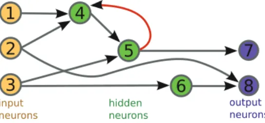
Fig. 3 Example of neural network with three input neurons, three hidden neurons, two output

neurons, and nine connections. One feedback connection (5→4) creates a cycle. Therefore, this is a recurrent NN. If that connection was removed, the network would be feed-forward only

Chapter2: A brief introduction to probabilistic machine learning and its relation to neuroscience.

In Chap.2, Trappenberg provides an overview of the most important ideas in modern machine learning, such as support vector machines and Bayesian networks. Meant as an introduction to the probabilistic formulation of machine learning, this chapter outlines a contemporary view of learning theories across three main paradigms: unsupervised learning, close to certain developmen-tal aspects of an organism, supervised learning, and reinforcement learning viewed as an important generalization of supervised learning in the temporal domain. Beside general comments on organizational mechanisms, the author discusses the relations between these learning theories and biological analo-gies: unsupervised learning and the development of filters in early sensory cor-tical areas, synaptic plasticity as the physical basis of learning, and research that relates models of basal ganglia to reinforcement learning theories. He also argues that, while lines can be drawn between development and learning to distinguish between different scientific camps, this distinction is not as clear as it seems since, ultimately, all model implementations have to be reflected by some morphological changes in the syste [279].

In this book, we focus on neural networks (NNs). Of all the machine learning algorithms, NNs provide perhaps the most direct analogy with the nervous system. They are also highly effective as engineering systems, often achieving state-of-the-art results in computer vision, signal processing, speech recognition, and many other areas (see [113] for an introduction). In what follows, we introduce a summary of a few concepts and terminology.

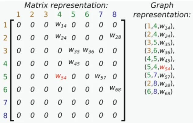
For our purposes, a neural network consists of a graph of neurons indexed by i. A connection i → j between two neurons is directed and has a weight wi j. Typically,

input neurons are application-specific (for example, sensors), output neurons are desired responses (for example, actuators or categories), and hidden neurons are information processing units located in-between (Fig.3).

Fig. 4 Two representations for the neural network of Fig.3

A neural network typically processes signals propagating through its units: a vector of floating-point numbers, s, originates in input neurons and resulting signals are transmitted along the connections. Each neuron j generates an output value vj

by collecting input from its connected neighbours and computing a weighted sum via an activation function, ϕ:

vj(s) =ϕ   # i | (i → j ) wi jvi(s)  

where ϕ(x) is often a sigmoid function, such as tanh(x), making the output nonlinear. For example, in the neural network of Fig.3, the output of neuron 8 can be written in terms of input signals v1,v2,v3as follows:

v8(s) =ϕ(w28v2+w68v6) =ϕ(w28v2+w68ϕ(w36v3))

Graph topologies without cycles are known as feedforward NNs, while topologies with cycles are called recurrent NNs. The former are necessarily stateless machines, while the latter might possess some memory capacity. With sufficient size, even simple feed-forward topologies can approximate any continuous function [44]. It is possible to build a Turing machine in a recurrent NN [260].

A critical question in this chapter concerns the representation format of such a net-work. Two common representations are adjacency matrices, which list every possible connection between nodes, and graph-based representations, typically represented as a list of nodes and edges (Fig.4). Given sufficient space, any NN topology and set of weights can be represented in either format.

Neural networks can be used to solve a variety of problems. In classification or regression problems, when examples of input-output pairs are available to the net-work during the learning phase, the training is said to be supervised. In this scenario, the fitness function is typically a mean square error (MSE) measured between the

network outputs and the actual outputs over the known examples. With feedback available for each training signal sent, NNs can be trained through several means, most often via gradient descent (as in the “backpropagation” algorithm). Here, a error or “loss function” E is defined between the desired and actual responses of the network, and each weight is updated according to the derivative of that function:

wi j(t +1) = wi j(t ) −η

∂ E ∂wi j

where η is the learning rate. Generally, this kind of approach assumes a fixed topology and its goal is to optimize the weights.

On the other hand, unsupervised learning concerns cases where no output samples are available and data-driven self-organization mechanisms are at work, such as Hebbian learning. Finally, reinforcement learning (including neuroevolution) is con-cerned with delayed, sparse and possibly noisy rewards. Typical examples include robotic control problems, decision problems, and a large array of inverse problems in engineering. These various topics will be discussed later.

1.3.3 Brain-Like AI: What’s Missing?

It is generally agreed that, at present, artificial intelligence (AI) is not “brain-like”. While AI is successful at many specialized tasks, none of them shows the versatil-ity and adaptabilversatil-ity of animal intelligence. Several authors have compiled a list of “missing” properties, which would be necessary for brain-like AI. These include: the capacity to engage in a behavioural tasks; control via a simulated nervous sys-tem; continuously changing self-defined representations; and embodiment in the real world [165,253,263,292]. Embodiment, especially, is viewed as critical because by exploiting the richness of information contained in the morphology and the dynamics of the body and the environment, intelligent behaviour could be generated with far less representational complexity [228,291].

The hypothesis explored in this book is that the missing feature is development. The brain is not built from a blueprint; instead, it grows in situ from a complex multicellular process, and it is this adaptive growth process that leads to the adap-tive intelligence of the brain. Our goal is not to account for all properties observed in nature, but rather to identify the relevance of a developmental approach with

respect to an engineering objectivedriven by performance alone. In the remainder of

this chapter, we review several approaches incorporating developmentally inspired strategies into artificial neural networks.

2 Artificial Development

There are about 1.5 million known species of multicellular organisms, representing an extraordinary diversity of body plans and shapes. Each individual grows from the division and self-assembly of a great number of cells. Yet, this developmental

process also imposes very specific constraints on the space of possible organisms, which restricts the evolutionary branches and speciation bifurcations. For instance, bilaterally symmetric cellular growth tends to generate organisms possessing pairs of limbs that are equally long, which is useful for locomotion, whereas asymmetrical organisms are much less frequent.

While the “modern synthesis” of genetics and evolution focused most of the attention on selection, it is only during the past decade that analyzing and under-standing variation by comparing the developmental processes of different species, at both embryonic and genomic levels, became a major concern of evolutionary development, or “evo-devo”. To what extent are organisms also the product of self-organized physicochemical developmental processes not necessarily or always con-trolled by complex underlying genetics? Before and during the advent of genetics, the study of developmental structures had been pioneered by the “structuralist” school of theoretical biology, which can be traced back to Goethe, D’Arcy Thompson, and Waddington. Later, it was most actively pursued and defended by Kauffman [150] and Goodwin [98] under the banner of self-organization, argued to be an even greater force than natural selection in the production of viable diversity.

By artificial development (AD), also variously referred to as artificial embryogeny, generative systems, computational ontogeny, and other equivalent expressions (see early reviews in [107,265]), we mean the attempt to reproduce the constraints and effects of self-organization in automated design. Artificial development is about creating a growth-inspired process that will bias design outcomes toward useful forms or properties. The developmental engineer engages in a form of “meta-design” [63], where the goal is not to design a system directly but rather set a framework in which human design or automated search will specify a process that can generate a desired result. The benefits and effectiveness of development-based design, both in natural and artificial systems, became an active topic of research only recently and are still being investigated.

Assume for now that our goal is to generate a design which maximizes an objective function, o: Φ → Rn_{, where Φ is the “phenotypic” space, that is, the space of}

potential designs, and Rn_{is a collection of performance assessments, as real values,}

with n ≥ 1 (n = 1 denotes a single-objective problem, while n > 1 denotes a multiobjective problem). A practitioner of AD will seek to generate a lower-level “genetic” space Γ , a space of “environments” E in which genomes will be expressed, and a dynamic process δ that transforms the genome into a phenotype:

Γ ×E−→ Φδ −→o Rn

In many cases, only one environment is used, usually a trivial or empty instance from the phenotypic space. In these cases, we simply write:

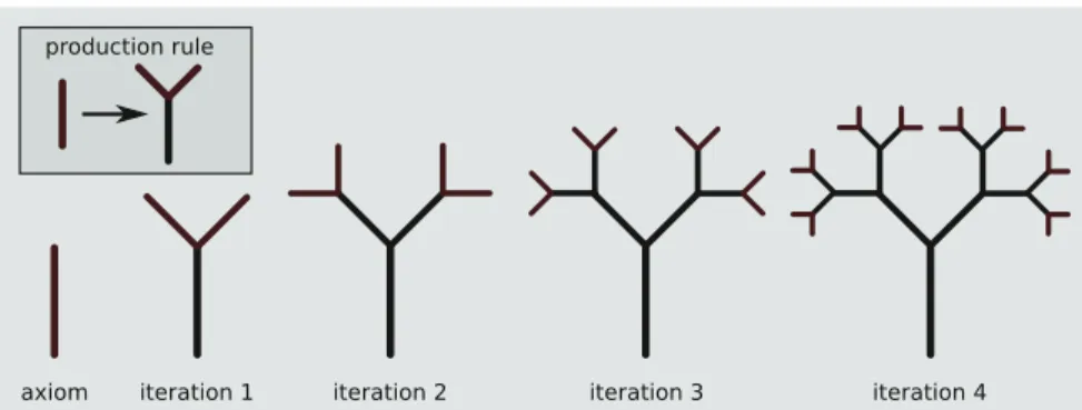
Fig. 5 Visualization of an L-System. Top-left a single production rule (the “genome”).

Bottom-leftthe axiom (initial “word”). Recursive application of the production rule generates a growing structure (the “phenotype”). In this case, the phenotype develops exponentially with each application of the production rule

The dynamic process δ is inspired by biological embryogenesis, but need not resem-ble it. Regardless, we will refer to it as growth or development, and to the quadruple (Γ ,E ,δ, Φ) as an AD system.

Often, the choice of phenotypic space Φ is dictated by the problem domain. For instance, to design neural networks, one might specify Φ as the space of all adjacency matrices, or perhaps as all possible instances of some data structure corresponding to directed, weighted graphs. Or to design robots, one might define Φ as all pos-sible lattice configurations of a collection of primitive components and actuators. Sometimes there is value in restricting Φ, for example to exclude nonsensical or dangerous configurations. It is the engineer’s task to choose an appropriate Φ and to “meta-design” the Γ , E, and δ parts that will help import the useful biases of biological growth into evolved systems.

A famous class of AD systems are the so-called L-Systems. These are formal grammars originally developed by Lindenmayer as a means of generating model plants [231]. In their simplest form, they are context-free grammars, consisting of a starting symbol, or “axiom”, a collection of variables and constants, and at most one production rule per variable. By applying the production rules to the axiom, a new and generally larger string of symbols, or “word”, is created. Repeated application of the production rules to the resulting word simulates a growth process, often leading to gradually more complex outputs. One such grammar is illustrated in Fig.5, where a single variable (red stick) develops into a tree-like shape. In this case, the space of phenotypes Φ is the collection of all possible words (collections of sticks), the space of genotypes Γ is any nonambiguous set of context-free production rules, the environment E is the space in which a phenotype exists (here trivially 2D space), and the dynamic process δ is the repeated application of the rules to a given phenotype. There are several important aspects to the meta-design of space of representations Γ and growth process δ. Perhaps the most critical requirement is that the chosen enti-ties be “evolvable”. This term has many definitions [129] but generally means that

Fig. 6 A mutation of the production rule in Fig.5, and the output after four iterations of growth

producion rule

Fig. 7 McCormack’s evolved L-Systems, inspired by, but exaggerating, Australian flora

the space of representations should be easily searchable for candidates that optimize some objective. A generally desirable trait is that small changes in a representation should lead to small changes in the phenotype—a “gentle slope” allowing for incre-mental search techniques. In AD systems, however, due to the nonlinear dynamic properties of the transformation process, it is not unusual for small genetic changes to have large effects on the phenotype [87].

For instance, consider in Fig.6 a possible mutation of the previous L-System. Here, the original genome has undergone a small change, which has affected the resulting form. The final phenotypes from the original and the mutated version are

similar in this case: they are both trees with an identical topology. However, it is not difficult to imagine mutations that would have catastrophic effects, resulting in highly different forms, such as straight lines or self-intersections. Nonlinearity of the genotype-to-phenotype mapping δ can be at the same time a strength and a weakness in design tasks.

There is an important distinction to be made here between our motivations and those of systems biology or computational neuroscience. In AD, we seek means of creating engineered designs, not simulating or reproducing biological phenomena. Perhaps this is best illustrated via an example: McCormack, a computational artist, works with evolutionary computation and L-Systems (Fig.7). Initially, this involved the generation of realistic models of Australian flora. Later, however, he continued to apply evolutionary methods to create exaggerations of real flora, artefacts that he termed “impossible nature” [187, 188]. McCormack’s creations retain salient properties of flora, especially the ability to inspire humans, but do not model any existing organism.

2.1 Why Use Artificial Development?

Artificial development is one way of approaching complex systems engineering, also called “emergent engineering” [282]. It has been argued that the traditional state-based approach in engineering has reached its limits, and the principles under-lying complex systems—self-organization, nonlinearity, and adaptation—must be accommodated in new engineering processes [11, 203]. Incorporating complex systems into our design process is necessary to overcome our present logjam of complexity, and open new areas of productivity. Perhaps the primary reason for the interest in simulations of development is that natural embryogenesis is a practical example of complex systems engineering, one which achieves designs of scale and functionality that modern engineers aspire to. There are several concrete demonstra-tions of importing desirable properties from natural systems into artificial counter-parts. The key property of evolvability, which we have already discussed, is linked to a notion of scalability. Other related properties include robustness via self-repair and plasticity.

2.1.1 Scalability

Perhaps the best studied property of AD systems is the ability to scale to several sizes. This is a consequence of a general decoupling of the complexity of the genome (what we are searching for) from the phenotype (the final product). In many models, the size of the phenotype is controlled via a single parameter, which can be the number of repetitions of a module, the number of iterations in an L-System, or a single variable

controlling the amount of available resources. In these cases, a minimal change in the size of the genome might have exponential effects on the size of the resulting phenotype.

This property—the capacity to scale—brings to mind the notion of “Kolmogorov complexity”, or the measurement of the complexity of a piece of data by the shortest computer program that generates it. With the decision to use AD, we make the assumption that there exists a short computer program that can generate our desired data, i.e. that the Kolmogorov complexity of our problem is small. This implies that AD will succeed in cases where the data to be generated is sufficiently large and non-random. Unfortunately, in the general case, finding such a program for some given data is an uncomputable problem, and to date there is no good approximation other than enumerating all possible programs, a generally untenable solution [173]. In many highly relevant domains of application, the capacity for scaling has been successfully demonstrated by AD systems. Researchers will often compare their AD model to a direct encoding model, in which each component of the solution is specified in the genome independently. Abstract studies have confirmed our intuition that AD systems are often better for large phenotypes and nonrandom data [40,

108]. This has also been demonstrated in neural networks [86, 104, 153], virtual robotics [161]; engineering design [127], and other domains [17,243].

2.1.2 Robustness and Self-repair

Another desirable property of biological systems is the capacity for robustness. By this, we mean a “canalization” or the fact that a resulting phenotype is resistant to environmental perturbations, whether they are obstacles placed in the path of a developing organism, damage inflicted, or small changes to external factors affecting cellular expression, such as temperature or sources of nutrient. In biology, this ability is hypothesized to result from a huge number of almost identical cells, a redundancy creating tolerance toward differences in cellular arrangement, cell damage, or the location of organizers [152]. Several AD systems have been shown to import robust-ness, which can be selected for explicitly [18]. More interestingly, robustness is often imported without the inclusion of selection pressure [86,161,243]. In many cases, this property seems to be a natural consequence of the use of an adaptive growth process as a design step.

An extreme example of robustness is the capacity for self-repair. Many authors have conducted experiments with AD systems in which portions of an individual are damaged (e.g. by scrambling or removing components). In these cases, organisms can often self-repair, reconfiguring themselves to reconstruct the missing or altered portions and optimize the original objective. For instance, this has been demonstrated in abstract settings [5,42,145,197], digital circuits [224], and virtual robotics [275]. Interestingly, in most of these cases, the self-repair capacity is not explicitly selected for in the design stage.

2.1.3 Plasticity

Another property of AD systems is plasticity, also referred to as polymorphism or polyphenism (although these terms are not strictly equivalent). By this, we mean the ability of organisms to be influenced by their environment and adopt as a result any phenotype from a number of possibilities. Examples in nature are legion [94], and most striking in the tendency of plants to grow toward light or food, or the ability of nervous systems to adapt to new stimuli. While robustness means reaching the same genotype under perturbation, plasticity means reaching different phenotypes under perturbation. Both, however, serve to improve the ultimate fitess of the organism in a variety of environments.

In classical neural systems, plasticity is the norm and is exemplified by well-known training methods: Hebbian learning, where connections between neurons are reinforced according to their correlation under stimuli [114], and backpropagation, where connection weights are altered according to an error derivative associated with incoming stimuli [245]. These classic examples focus on synaptic structure, or the weighting of connections in some predetermined network topology. While this is certainly an element of natural self-organization, it is by no means a complete char-acterization of the role that plasticity plays in embryogenesis. Environmental stimuli in animal morphogenesis include other neural mechanisms, such as the constant re-formation and re-connection of synapses. Both selectivist and constructivist theories of brain development posit a central role for environmental stimuli in the generation of neural morphology. Furthermore, plasticity plays a major role in other develop-mental processes as well. In plants, the presence or absence of nutrients, light, and other cues will all but determine the coarse morphology of the resulting form. In animals, cues such as temperature, abundance of nutrients, mechanical stress, and available space are all strong influences. Indeed, the existence of plasticity is viewed as a strong factor in the evolvability of forms: for instance, plastic mechanisms in the development of the vascular system allow for a sort of “accidental adaptation”, where novel morphological structures are well served by existing genetic mecha-nisms for vasculogenesis, despite never being directly selected for in evolutionary history [99,177].

Most examples of artificial neural systems exploit plasticity mechanisms to tune parameters according to some set of “training” stimuli. Despite this, the use of envi-ronmentally induced plasticity in AD systems is rare. Only a few examples have shown that environmental cues can be used to reproduce plasticity effects com-monly seen in natural phenomena, such as: virtual plant growth [87,252], circuit design [280], or other scenarios [157,190]. In one case, Kowaliw et al. experimented with the growth of planar trusses, a model of structural engineering. They initially showed that the coarse morphology of the structures could be somewhat controlled by the choice of objective function—however, this was also a difficult method of morphology specification [163]. Instead, the authors experimented with external constraints, which consisted of growing their structures in an environment that had the shape of the desired morphology. Not only was this approach generally success-ful in the sense of generating usable structures of the desired overall shape, but it

also spontaneously generated results indicating evolvability. A few of the discovered genomes could grow successful trusses not only in the specific optimization envi-ronment but also in all the other experimental envienvi-ronments, thus demonstrating a capacity for accidental adaptation [162].

2.1.4 Other Desirable Natural Properties

Other desirable natural properties are known to occasionally result from AD systems. These include: graceful degradation, i.e. the capacity for systems performance to fail continuously with the removal of parts [18]; adaptation to previously unseen environ-ments, thought to be the result of repetitions of phenotypic patterns capturing useful regularities (see, for instance, Chap. 9 [206]); and the existence of “scafolding”, i.e. a plan for the construction of the design in question, based on the developmental growth plan [241].

2.2 Models of Growth

An AD system requires a means of converting a representation into a design. This conversion typically involves a dynamic process that generates an arrangement of “cells”, where these cells can stand for robotic components, structural members, neu-rons, and so on. Several models of multi-component growth have been investigated in detail:

• Induced representational bias: the designer adds a biologically inspired bias to an otherwise direct encoding. Examples include very simple cases, such as mirroring elements of the representation to generate symmetries in the phenotype [256], or enforcing a statistical property inspired by biological networks, such as the density of connections in a neural system [258].

• Graph rewriting: the phenotype is represented as a graph, the genome as a

col-lection of graph-specific actions, and growth as the application of rules from the genome to some interim graph. Examples of this paradigm include L-Systems and dynamic forms of genetic programming [109,122].

• Cellular growth models: the phenotype consists of a collection of cells on a lattice

or in continuous space. The genome consists of logic that specifies associations between cell neighbourhoods and cell actions, where the growth of a phenotype involves the sum of the behaviours of cells. Cellular growth models are sometimes based on variants of cellular automata, a well-studied early model of discrete dynamics [161,197]. This choice is informed by the success of cellular automata in the simulation of natural phenomena [56]. Other models involve more plausible physical models of cellular interactions, where cells orient themselves via inter-cellular physics [25,62,76,144,249]

• Reaction-diffusion models: due to Turing [281], they consist of two or more

simulated chemical agents interacting on a lattice. The chemical interactions are modelled as nonlinear differential equations, solved numerically. Here, sim-ple equations quickly lead to remarkable examsim-ples of self-organized patterns. Reaction-diffusion models are known to model many aspects of biological devel-opment, including overall neural organization [172, 259] and organismal behav-iour [47,298].

• Other less common but viable choices include: the direct specification of

dynamical systems, where the genome represents geometric components such as attractors and repulsors [267]; the use of cell sorting, or the simulation of ran-dom cell motion among a collection of cells with various affinities for attraction, which can be used to generate a final phenotype [107].

A major concern for designers of artificial development (and nearly all com-plex systems) is how to find the micro-rules which will generate a desired macro-scale pattern. Indeed, this problem has seen little progress despite several decades of research, and in the case of certain generative machines such as cellular automata, it is even known to be impossible [133]. The primary way to solve this issue is using a machine learner as a search method. Evolutionary computation is the general choice for this machine learner, mostly due to the flexibility of genomic representations and objective functions, and the capacity to easily incorporate conditions and heuris-tics. In this case, the phenotype of the discovered design solution will be an unpre-dictable, emergent trait of bottom-up design choices, but one which meets the needs of the objective function. Various authors have explored several means of ameliorat-ing this approach, in particular by controllameliorat-ing or predictameliorat-ing the evolutionary output [213,214].

2.3 Why Does Artificial Development Work?

The means by which development improves the evolvability of organisms is a critical question. In biology, the importance of developmental mechanisms in organismal organization has slowly been acknowledged. Several decades ago, Gould (contro-versially) characterized the role of development as that of a “constraint”, or a “fruit-ful channelling [to] accelerate or enhance the work of natural selection” [99]. Later authors envisioned more active mechanisms, or “drives” [7, 152]. More recently, discussion has turned to “increased evolvability”, partly in recognition that no sim-ple geometric or phenotypic description can presently describe all useful phenotypic biases [115]. At the same time, mechanisms of development have gained in impor-tance in theoretical biology, spawning the field of evo-devo [31] mentioned above, and convincing several researchers that the emergence of physical epigenetic cellular mechanisms capable of supporting robust multicellular forms was, in fact, the “hard” part of the evolution of today’s diversity of life [212].

Inspired by this related biological work, practitioners of artificial development have hypothesized several mechanisms as an explanation for the success of artificial development, or as candidates for future experiments:

• Regularities: this term is used ambiguously in the literature. Here, we refer to the

use of simple geometrically based patterns over space as a means of generating or biasing phenotypic patterns, for example relying on Wolpert’s notion of gradient-based positional information [295]. This description includes many associated biological phenomena, such as various symmetries, repetition, and repetition with variations. Regularities in artificial development are well studied and present in many models; arguably the first AD model, Turing’s models of chemical morpho-genesis, relied implicitly on such mechanisms through chemical diffusion [281]. A recent and popular example is the Compositional Pattern Producing Network (CPPN), an attempt to reproduce the beneficial properties of development without explicit multicellular simulation [266] (see also Sect.5.4and Chap. 5).

• Modularity: this term implies genetic reuse. Structures with commonalities are

routine in natural organisms, as in the repeated vertebrae of a snake, limbs of a centipede, or columns in a cortex [29]. As Lipson points out, modules need not even repeat in a particular organism or design, as perhaps they originate from a meta-processes, such as the wheel in a unicycle [174]. Despite this common con-ception, there is significant disagreement on how to define modularity in neural systems. In cognitive science, a module is a functional unit: a specialized and encapsulated unit of function, but not necessarily related to any particular low-level property of neural organization [89,233]. In molecular biology, modules are measured as either information-theoretic clusters [121], or as some measure of the clustering of network nodes [147,211, 289]. These sorts of modularity are implicated in the separation of functions within a structure, allowing for greater redundancy in functional parts, and for greater evolvability through the separa-tion of important funcsepara-tions from other mutable elements [229]. Further research shows that evolution, natural and artificial, induces modularity in some form, under pressures of dynamic or compartmentalized environments [23,24,39,121,147], speciation [82], and selection for decreased wiring costs [39]. In some cases, these same measures of modularity are applied to neural networks [23,39,147]. Beyond modularity, hierarchy (i.e. the recursive composition of a structure and/or function [64,124,174]) is also frequently cited as a possibly relevant network property. • Phenotypic properties: Perhaps the most literal interpretation of biological theory

comes from Matos et al., who argue for the use of measures on phenotypic space. In this view, an AD system promotes a bias on the space of phenotypic structures that can be reached, which might or might not promote success in some particular domain. By enumerating several phenotypic properties (e.g. “the number of cells produced”) they contrast several developmental techniques, showing the bias of AD systems relative to the design space [185]. While this approach is certainly capable of adapting to the problem at hand, it requires a priori knowledge of the interesting phenotypic properties—something not presently existing for large neural systems;

• Adaptive feedback and learning: Some authors posit adaptive feedback during

development as a mechanism for improved evolvability. The use of an explicit developmental stage allows for the incorporation of explicit cues in the resulting phenotype, a form of structural plasticity which recalls natural growth. These cues include not only a sense of the environment, as was previously discussed, but also interim indications of the eventual success of the developing organism. This latter notion, that of a continuous measure of viability, can be explicitly included in AD system, and has been shown in simple problems to improve efficacy and efficiency [12,157,158,190]. A specialized case of adaptive feedback is

learn-ing, by which is meant the reaction to stimuli by specialized plastic components

devoted to the communication and processing of inter-cellular signals. This impor-tant mechanism is discussed in the next section.

3 Artificial Neurogenesis

By artificial neurogenesis, we mean a developmentally inspired process that

gener-ates neural systems for use in a practical context. These contexts include tasks such

as supervised learning, computer vision, robotic control, and so on. The definition of developmentally inspired processes in this chapter is also kept broad on purpose: at this early stage, we do not want to exclude the possibility that aspects of our current understanding of development are spurious or replaceable.

An interesting early example of artificial neurogenesis is Gruau’s cellular

encod-ing[103]. Gruau works with directed graph structures: each neural network starts

with one input and one output node, and a hidden “mother” cell connected between them. The representation, or “genome”, is a tree encoding that lists the successive cell actions taken during development. The mother cell has a reading head pointed at the top of this tree, and executes any cellular command found there. In the case of a division, the cell is replaced with two connected children, each with reading heads pointed to the next node in the genome. Other cellular commands change registers inside cells, by adding bias or changing connections. A simple example is illustrated in Fig.8.

Through this graph-based encoding, Gruau et al. designed and evolved networks solving several different problems. Variants of the algorithm used learning as a mid-step in development and encouraged modularity in networks through the introduction of a form of genomic recursion [103,104]. The developed networks showed strong phenotypic organization and modularity (see Fig.9for samples).

3.1 The Interplay Between Development and Learning

A critical difference between artificial neurogenesis and AD is the emphasis on learn-ing in the latter. Through the modelllearn-ing of neural elements, a practitioner includes

Fig. 8 Simple example of a neural network generated via cellular encoding (adapted from [103]). On the left, an image of the genome of the network. On the right, snapshots of the growth of the neural network. The green arrows show the reading head of the active cells, that is, which part of the genome they will execute next. This particular network solves the XOR problem. Genomic recurrence (not shown) is possible through the addition of a recurrence node in the genomic tree

Fig. 9 Sample neural networks generated via cellular encoding: left a network solving the 21-bit parity problem; middle a network solving the 40-bit symmetry problem; right a network imple-menting a 7-input, 128-output decoder (reproduced with permission from [103])

any number of plasticity mechanisms that can effectively incorporate environmental information.

One such hypothetical mechanism requiring the interplay between genetics and epigenetics is the Baldwin effect [9]. Briefly, it concerns a hypothesized process that occurs in the presence of both genetic and plastic changes and accelerates evolution-ary progress. Initially, one imagines a collection of individuals distributed randomly over a fitness landscape. As expected, the learning mechanism will push some, or all, of these individuals toward local optima, leading to a population more optimally dis-tributed for non-genetic reasons. However, such organisms are under “stress” since they must work to achieve and maintain their epigenetically induced location in the fitness landscape. If a population has converged toward a learned optimum, then in subsequent generations, evolution will operate to lower this stress, by finding genetic

means of reducing the amount of learning required. Thus, learning will identify an optimum, and evolution will gradually adapt the genetic basis of the organism to fit the discovered optimum. While this effect is purely theoretical in the natural world, it has long been known that it can be generated in simple artificial organisms [120]. Accommodating developmental processes in these artificial models is a challenge, but examples exist [72,103]. Other theories of brain organization, such as displace-ment theory, have also been tentatively explored in artificial systems [70,71].

3.2 Why Use Artificial Neurogenesis?

There is danger in the assumption that all products of nature were directly selected for their contribution to fitness; this Panglossian worldview obscures the possibility that certain features of natural organisms are the result of non-adaptive forces, such as genetic drift, imperfect genetic selection, accidental survivability, side-effects of ontogeny or phylogeny, and others [100]. In this spirit, we note that while a computer simulation might show a model to be sufficient for the explanation of a phenomenon, it takes more work to show that it is indeed necessary. Given the staggering complex-ity of recent neural models, even a successful recreation of natural phenomena does not necessarily elucidate important principles of neural organization, especially if the reconstructed system is of size comparable to the underlying data source. A position of many practitioners working with bio-inspired neural models, as in artificial intel-ligence generally, is that an alternative path to understanding neural organization

is the bottom-up construction of intelligent systems. The creation of artefacts

capa-ble of simple behaviours that we consider adaptive or intelligent gives us a second means of “understanding” intelligent systems, a second metric through which we can eliminate architectural overfitting from data-driven models, and identify redundant features of natural systems.

A second feature of many developmental neural networks is the reliance on local communication. Practitioners of AD will often purposefully avoid global information (e.g. in the form of coordinate spaces or centralized controllers) in order to generate systems capable of emergent global behaviour from purely local interactions, as is the case in nature. Regardless of historic motivations, this attitude brings potential benefits in engineered designs. First, it assumes that the absence of global control contributes to the scalability of developed networks (a special form of the robust-ness discussed in Sect.2.1.1). Second, it guarantees that the resulting process can be implemented in a parallel or distributed architecture, ideally based on physically asynchronous components. Purely local controllers are key in several new engineer-ing application domains, for instance: a uniform array of locally connected hardware components (such as neuromorphic engineering), a collection of modules with lim-ited communication (such as a swarm of robots, or a collection of software modules over a network), or a group of real biological cells executing engineered DNA (such as synthetic biology).

3.3 Model Choices

A key feature in artificial neurogenesis is the level of simulation involved in the growth model. It can range from highly detailed, as is the case for models of cellular physics or metabolism, to highly abstract, when high-level descriptions of cellular groups are used as building blocks to generate form. While realism is the norm in computational neuroscience, simpler and faster models are typical in machine learn-ing. An interesting and open question is whether or not this choice limits the capacity of machine learning models to solve certain problems. For artificial neurogenesis, rel-evant design decisions include: spiking versus non-spiking neurons, recurrent versus feed-forward networks, the level of detail in neural models (e.g. simple transmission of a value versus detailed models of dendrites and axons), and the sensitivity of neural firing to connection type and location.

Perhaps the most abstract models come from the field of neuroevolution, which relies on static feed-forward topologies and nonspiking neurons. For instance, Stan-ley’s HyperNEAT model [49] generates a pattern of connections from another lattice of feed-forward connections based on a composition of geometric regularities. This model is a highly simplified view of neural development and organization, but can be easily evolved (see Chap. 5, [48]). A far more detailed model by Khan et al. [151] provides in each neuron several controllers that govern neural growth, the synap-togenesis of dendrites and axons, connection strength, and other factors. Yet, even these models are highly abstract compared to other works from computational neu-roscience, such as the modelling language of Zubler et al. [311]. The trade-offs associated with this level of detailed modelling are discussed in depth by Miller (Chap. 8, [198]).

Assuming that connectivity between neurons depends on their geometric loca-tion, a second key question concerns the level of stochasticity in the placement of those elements. Many models from computational neuroscience assume that neural positions are at least partially random, and construct models that simply overlay pre-formed neurons according to some probability law. For instance, Cuntz et al. posit that synapses follow one of several empirically calculated distributions, and con-struct neural models based on samples from those distributions [41]. Similarly, the Blue Brain project assumes that neurons are randomly scattered: this model does, in fact, generate statistical phenomena which resemble actual brain connectivity pat-terns [116].

A final key decision for artificial neurogenesis is the level of detail in the simulation of neural plasticity. These include questions such as:

• Is plasticity modelled at all? In many applications of neuroevolution (Sect.4.3), it is not: network parameters are determined purely via an evolutionary process. • Does plasticity consist solely of the modification of connection weights or firing

rates? This is the case in most classical neural networks, where a simple, almost arbitrary network topology is used, such as a multilayer perceptron. In other cases, connection-weight learning is applied to biologically motivated but static network topologies (Sects.4.1and4.2, Chap.7 [13]).