On dependence consistency of CoVaR and some other systemic risk measures

Georg Mainik and Eric Schaanning*

On dependence consistency of CoVaR and

some other systemic risk measures

Abstract: This paper is dedicated to the consistency of systemic risk measures with

respect to stochastic dependence. It compares two alternative notions of Condi-tional Value-at-Risk (CoVaR) available in the current literature. These notions are both based on the conditional distribution of a random variable𝑌given a stress event for a random variable𝑋, but they use different types of stress events. We de-rive representations of these alternativeCoVaRnotions in terms of copulas, study their general dependence consistency and compare their performance in several stochastic models. Our central finding is that conditioning on𝑋 ≥ VaR_𝛼(𝑋)gives a much better response to dependence between𝑋and𝑌than conditioning on

𝑋 = VaR_𝛼(𝑋). We prove general results that relate the dependence consistency ofCoVaRusing conditioning on𝑋 ≥ VaR_𝛼(𝑋)to well established results on con-cordance ordering of multivariate distributions or their copulas. These results also apply to some other systemic risk measures, such as the Marginal Expected Shortfall (MES) and the Systemic Impact Index (SII). We provide counterexam-ples showing thatCoVaRbased on the stress event𝑋 = VaR_𝛼(𝑋)is not depen-dence consistent. In particular, if(𝑋, 𝑌)is bivariate normal, thenCoVaRbased on

𝑋 = VaR_𝛼(𝑋)is not an increasing function of the correlation parameter. Similar issues arise in the bivariate𝑡model and in the model with𝑡margins and a Gum-bel copula. In all these cases,CoVaRbased on𝑋 ≥ VaR_𝛼(𝑋)is an increasing function of the dependence parameter.

Keywords: Systemic risk measures, conditional Value-at-Risk (CoVaR), Risk spillover, dependence consistency, stochastik ordering.

AMS 2010: 91G70, 62H20, 91G99, 91B82, 60E15

||

*Corresponding Author: Eric Schaanning, Mathematical Finance Section, Department of

Math-ematics, Imperial College London, 180 Queen’s Gate, SW7 2AZ, London, United Kingdom, e-mail: e.schaanning12@imperial.ac.uk

Georg Mainik: RiskLab, Department of Mathematics, ETH Zurich, Raemistrasse 101, 8092

1 Introduction

The present paper studies the notion of Conditional Value-at-Risk (CoVaR) intro-duced byAdrian and Brunnermeier(2008) as a dependence adjusted version of Value-at-Risk (VaR). The general idea behindCoVaRis to use the conditional dis-tribution of a random variable𝑌representing a particular financial institution (or the entire financial system) given that another institution, represented by a ran-dom variable𝑋, is under stress.CoVaRrepresents one of the major threads in the current regulatory and scientific discussion of systemic risk, which significantly intensified after the recent financial crisis. The current discussion on systemic risk measurement is far from being concluded, and the competing methodologies are still under development. In addition to systemic risk measures (cf.Acharya

et al.(2010), Adrian and Brunnermeier(2008,2010), Girardi and Ergün(2013),

Goodhart and Segoviano(2008), Huang et al.(2012),Zhou(2010)), related topics

include the structure of interbank networks, e.g.,Boss et al.(2004), Cont et al.

(2013), models explaining how systemic risk is created, e.g.,Choi and Douady

(2012), Ibragimov and Walden(2007), and attribution of systemic risk charges

within a financial system, as discussed inStaum(2012), Tarashev et al.(2010). Also the recent survey byBisias et al.(2012) provides an extensive overview of different measures in the literature.

Our contribution addresses the consistency of systemic risk measures with re-spect to the dependence in the underlying stochastic model. In the case ofCoVaR

we give a strong indication for the choice of the stress event for the conditioning random variable𝑋. There are two alternative definitions ofCoVaRin the current literature. The original definition inAdrian and Brunnermeier(2008,2009,2010) is derived from the conditional distribution of𝑌given that𝑋 = VaR_𝛼(𝑋). The second one uses conditioning on𝑋 ≥ VaR_𝛼(𝑋). This modification was proposed

by Girardi and Ergün(2013) to improve the compatibility ofCoVaRwith

non-parametric estimation methods. For similar reasons, such as continuity and bet-ter compatibility with discrete distributions, conditioning on𝑋 ≥ VaR_𝛼(𝑋)was also favoured byKlyman(2011) for bothCoVaRand Conditional Expected Short-fall (CoES). Finally, it is remarkable that most competitors ofCoVaR(cf.Acharya et al.(2010), Goodhart and Segoviano(2008), Huang et al.(2012), Zhou(2010)) use conditioning on𝑋 ≥ VaR_𝛼(𝑋)as well. This approach goes in line with the general concept of stress scenarios discussed inBalkema and Embrechts(2007).

Our results show that conditioning on𝑋 ≥ VaR_𝛼(𝑋)has great advantages for dependence modelling. We prove that this modification ofCoVaRmakes it respond consistently to dependence parameters in many important stochastic models, whereas the original definition ofCoVaRfails to do so. The

counterex-amples even include the bivariate Gaussian model, where the originalCoVaRis decreasing with respect to the correlation𝜌 := corr(𝑋, 𝑌) for𝜌 > 1/√2. Thus,

CoVaRbased on{𝑋 = VaR_𝛼(𝑋)}fails to detect systemic risk when it is most pro-nounced; and we also found this kind of inconsistency in other examples. On the other hand, our findings for the modifiedCoVaRrelate its dependence consis-tency to concordance ordering of multivariate distributions or related copulas. This may explain the comparative results inGauthier et al.(2012), whereCoVaR

stood somewhat apart from its competitors. Moreover, it gives the modified notion ofCoVaRa solid mathematical basis.

BesidesCoVaR, we also discuss extensions to Conditional Expected Short-fall (CoES). It turns out that the dependence inconsistency or dependence consis-tency of the alternativeCoVaRnotions is propagated to the corresponding defini-tions ofCoES. The dependence consistency results forCoVaRandCoES, based on the stress scenario𝑋 ≥ VaR_𝛼(𝑋), also apply to the Marginal Expected Short-fall (MES) defined inAcharya et al.(2010) and to the Systemic Impact Index (SII) introduced inZhou(2010).

The paper is organized as follows. Basic notation and alternative definitions of

CoVaRandCoESare given in Section2. In Section3we present the general math-ematical results, including representations ofCoVaRin terms of copulas and con-sistency of the modifiedCoVaRorCoESwith respect to dependence character-istics. Section4contains a detailed comparison of the original and the modified

CoVaRin three different models: the bivariate normal, the bivariate𝑡distribution, and a bivariate distribution with𝑡margins and a Gumbel copula. Conclusions are stated in Section5.

2 Basic definitions and properties

Let𝑋and𝑌be random variables representing the profits and losses of two finan-cial institutions, such as banks. Focusing on risks, let𝑋and𝑌be random loss variables, so that positive values of𝑋and𝑌represent losses, whereas the gains are represented by negative values.

The issues of contagion and systemic stability raise questions for the joint probability distribution of𝑋and𝑌:

𝐹_𝑋,𝑌(𝑥, 𝑦) := P(𝑋 ≤ 𝑥, 𝑌 ≤ 𝑦).

The corresponding marginal distributions will be denoted by𝐹_𝑋and𝐹_𝑌. Provided a method to quantify the loss or gain of the entire financial system,𝐹_𝑋,𝑌can also represent the joint loss distribution of a bank𝑋and the system𝑌.

In the current banking regulation framework (Basel II and the so-called Basel 2.5), the calculation of risk capital is based on measuring risk of each institution separately, with Value-at-Risk (VaR) as a risk measure. The Value-at-Risk of a ran-dom loss𝑋at the confidence level𝛼 ∈ (0, 1)is the𝛼-quantile of the loss distribu-tion𝐹_𝑋(cf.McNeil et al.(2005, Definition 2.10)). That is,

VaR_𝛼(𝑋) = 𝐹_𝑋←(𝛼),

where𝐹_𝑋←(𝑦) := inf{𝑥 ∈ ℝ : 𝐹_𝑋(𝑥) ≥ 𝑦}is the generalized inverse of𝐹_𝑋. The most common values of𝛼are0.95and0.99.

For continuous and strictly increasing𝐹_𝑋the generalized inverse𝐹_𝑋← coin-cides with the inverse function𝐹_𝑋−1of𝐹_𝑋. In this case one hasVaR_𝛼(𝑋) = 𝐹_𝑋−1(𝛼)

for𝛼 ∈ (0, 1). For a thorough discussion of generalized inverse functions we refer

toEmbrechts and Hofert(2010).

In the present paper we discuss two alternative approaches to adjustVaRto dependence between𝑋and𝑌. This is achieved by conditioning the distribution of𝑌on a stress scenario for𝑋. These two notions appear in the recent literature under the name Conditional Value-at-Risk (CoVaR), but they use different kinds of stress scenarios. The original notion was introduced byAdrian and Brunnermeier

(2008,2009,2010) and will henceforth be denoted byCoVaR=. The alternative definition was proposed byGirardi and Ergün(2013). We denote it byCoVaR.

Definition 2.1. CoVaR=_𝛼,𝛽(𝑌|𝑋) := VaR_𝛽(𝑌|𝑋 = VaR_𝛼(𝑋)); CoVaR_𝛼,𝛽(𝑌|𝑋) := VaR_𝛽(𝑌|𝑋 ≥ VaR_𝛼(𝑋)).

The computation ofCoVaR=requires the knowledge of𝐹_{𝑌|𝑋=VaR}

𝛼(𝑋). If𝐹𝑋,𝑌has

a density𝑓_𝑋,𝑌, then𝑓_𝑋(𝑥) = ∫_−∞∞ 𝑓_𝑋,𝑌(𝑥, 𝑦)𝑑𝑦is a density of𝐹_𝑋, and

𝐹_{𝑌|𝑋=VaR}

𝛼(𝑋)(𝑦) = ∫𝑦

−∞𝑓𝑋,𝑌(VaR𝛼(𝑋), 𝑡) d𝑡

𝑓_𝑋(VaR_𝛼(𝑋)) ,

provided that𝑓_𝑋(VaR_𝛼(𝑋)) > 0. In some models, such as elliptical distributions,

𝐹_{𝑌|𝑋=VaR}

𝛼(𝑋)is known explicitly. In general, however, computation of𝐹𝑌|𝑋=VaR𝛼(𝑋)

requires numerical integration.

Conditioning on𝑋 ≥ VaR_𝛼(𝑋)is less technical. The definition ofVaR_𝛼(𝑋)

implies thatP(𝑋 ≥ VaR_𝛼(𝑋)) ≥ 1−𝛼, so that elementary conditional probabilities are well defined. In particular, if𝐹_𝑋is continuous, then

𝐹_{𝑌|𝑋≥VaR}

𝛼(𝑋)(𝑦) =

P(𝑌 ≤ 𝑦, 𝑋 ≥ VaR_𝛼(𝑋))

1 − 𝛼 .

Moreover, conditioning on events with positive probabilities is advantageous in statistical applications, including model fitting and backtesting. This is the major

reason why the original notion ofCoVaR=was modified toCoVaRinGirardi and Ergün(2013).

A straightforward extension fromCoVaR to Conditional Expected Shortfall (CoES) is based on the representationES_𝛽(𝑌) = _1−𝛽1 ∫1

𝛽VaR𝑡(𝑌)d𝑡. Definition 2.2. CoES_𝛼,𝛽(𝑌|𝑋) := 1 1 − 𝛽 1 ∫ 𝛽 CoVaR_𝛼,𝑡(𝑌|𝑋)d𝑡, (2.1) CoES=_𝛼,𝛽(𝑌|𝑋) := 1 1 − 𝛽 1 ∫ 𝛽 CoVaR=_𝛼,𝑡(𝑌|𝑋)d𝑡. (2.2)

Remark 2.3. (a) In precise mathematical terms,CoVaR_𝛼,𝛽= andCoVaR_𝛼,𝛽are the

𝛽-quantiles of the conditional distributions𝐹_{𝑌|𝑋=VaR}

𝛼(𝑋)and𝐹𝑌|𝑋≥VaR𝛼(𝑋): CoVaR=_𝛼,𝛽(𝑌|𝑋) = 𝐹_{𝑌|𝑋=VaR}←

𝛼(𝑋)(𝛽); CoVaR_𝛼,𝛽(𝑌|𝑋) = 𝐹_{𝑌|𝑋≥VaR}←

𝛼(𝑋)(𝛽).

(b) InAdrian and Brunnermeier(2008,2010), Girardi and Ergün(2013), Jaeger-Ambrozewicz(2010), the authors work with a common confidence level for𝑋

and𝑌, i.e., the special case𝛼 = 𝛽. Similarly to the notation used there, we will omit𝛽if𝛽 = 𝛼and writeCoVaR_𝛼instead ofCoVaR_𝛼,𝛼if it does not lead to

confusion. However, the definition ofCoESrequires separate confidence levels

for𝑋and𝑌in the integrandCoVaR_𝛼,𝑡(𝑌|𝑋).

(c) SinceCoES_𝛼,𝛽(𝑌|𝑋) = ES_𝛽(𝑍)for a random variable𝑍 ∼ 𝐹_{𝑌|𝑋≥VaR}

𝛼(𝑋), the

co-herence ofESin the sense ofArtzner et al.(1999) is inherited byCoES_𝛼,𝛽for all𝛼, 𝛽 ∈ (0, 1). The central point here is subadditivity, which is understood as

CoES_𝛼,𝛽(𝑌 + 𝑌󸀠|𝑋) ≤ CoES_𝛼,𝛽(𝑌|𝑋) + CoES_𝛼,𝛽(𝑌󸀠|𝑋)

for any random variables(𝑌, 𝑌󸀠, 𝑋)defined on the same probability space.

(d) In Adrian and Brunnermeier (2008, 2010), CoES is defined as E[𝑌|𝑌 ≥ CoVaR_𝛼,𝛼= (𝑌|𝑋)]. Note that this definition replaces the stress scenario{𝑋 = VaR_𝛼(𝑋)}by{𝑌 ≥ CoVaR=_𝛼,𝛼(𝑌|𝑋)}, which is not directly related to𝑋. Com-pared toCoES=_𝛼,𝛽(𝑌|𝑋), this definition is quite unnatural. Moreover, it does not guarantee coherence, which is the central property of Expected Shortfall.

(e) The notion of Marginal Expected Shortfall (MES) introduced inAcharya et al.

(2010) is closely related toCoVaRandCoES. It is defined as

where𝑋 := ∑𝑑_𝑖=1𝑌_𝑖is the financial system and𝑌 := 𝑌_𝑖for some𝑖is an

institu-tion. The idea behindMESis to quantify the insurance premia corresponding

to bail-outs which become necessary when the entire financial system is close

to a collapse. The major economic difference betweenMESandCoVaRis the

role of𝑋and𝑌. WithMES, the conditioning random variable𝑋is the system,

and the target random variable𝑌is a part of the system. In the original work on

CoVaR,𝑌is the system, and𝑋is a part of it.

On the mathematical level,MESandCoVaRorCoESare quite close to each

other. It is easy to see that

MES_𝛼(𝑌|𝑋) = 1 ∫ 0 𝐹_{𝑌|𝑋≥VaR}← 𝛼(𝑋)(𝑡)𝑑𝑡 = 1 ∫ 0 CoVaR_𝛼,𝑡(𝑌|𝑋)𝑑𝑡.

In view of (2.1), one could also writeMES_𝛼(𝑌|𝑋) = CoES_𝛼,0(𝑌|𝑋).

(f) InKlyman(2011),CoVaR_𝛼,𝛽andCoES_𝛼,𝛽in the sense of Definitions2.1and2.2

are calledDistVaRandDistES. Besides the different naming, the definitions

are essentially the same, and these notions are also compared toCoVaR=and

CoES=. However, the comparison inKlyman(2011) is concentrated on general

representations, compatibility with discrete, e.g., empirical, distributions, and the behaviour in the bivariate Black-Scholes model. As far as we are aware, a study of consistency with respect to dependence parameters has been missing so far.

The introduction of CoVaR= in Adrian and Brunnermeier(2008) aims not at

CoVaR=itself, but at the contribution of a particular financial institution to the systemic risk. InAdrian and Brunnermeier(2008),CoVaR=is used to construct a risk contribution measure that should quantify how a stress situation for an institution𝑋affects the system (or another institution)𝑌. The authors propose

CoVaR= 𝛼,𝛽(𝑌|𝑋)

VaR𝛽(𝑌) − 1

as a systemic risk indicator. InAdrian and Brunnermeier(2009), the systemic risk measure is modified to

ΔCoVaR=_𝛼,𝛽(𝑌|𝑋) := CoVaR=_𝛼,𝛽(𝑌|𝑋) − VaR_𝛽(𝑌). (2.3)

InAdrian and Brunnermeier(2010), the centring termVaR_𝛽(𝑌)representing the

risk of𝑌in an unstressed state is replaced by the conditionalVaRof𝑌given that

𝑋is equal to its median:

ΔmedCoVaR=_𝛼,𝛽(𝑌|𝑋) := CoVaR=_𝛼,𝛽(𝑌|𝑋) − VaR_𝛽(𝑌|𝑋 = med(𝑋)) (2.4) to remedy some inconsistencies observed in a comparison ofCoVaR=across dif-ferent models.

Unfortunately, the centring in (2.3) is not the only reason whyΔCoVaR=can give a biased view of dependence between𝑋and𝑌. The results presented be-low demonstrate that there is a more fundamental issue that cannot be solved by modifyingΔCoVaR=toΔmedCoVaR=or taking any other centring term. The pri-mary deficiency ofΔCoVaR=is that the underlying stress scenario𝑋 = VaR_𝛼(𝑋)

is too selective and over-optimistic. If, for instance,𝐹_𝑋is continuous, thenP(𝑋 = VaR_𝛼(𝑋)) = 0, so that this particular event actually never occurs. Generally speak-ing, the ability ofCoVaR=,ΔCoVaR=, orΔmedCoVaR=to describe the influence of𝑋on𝑌 strongly depends on how well𝐹_{𝑌|𝑋=VaR}

𝛼(𝑋)approximates𝐹𝑌|𝑋=𝑥 for 𝑥 ≥ VaR_𝛼(𝑋). As shown in Section4, this approximation fails even in very ba-sic models, and it typically underestimates the contagion from𝑋to𝑌.

3 General results

We begin with representations ofCoVaR=andCoVaRin terms of copulas. It is well known that any bivariate distribution function𝐹_𝑋,𝑌admits the decomposi-tion

𝐹_𝑋,𝑌(𝑥, 𝑦) = 𝐶(𝐹_𝑋(𝑥), 𝐹_𝑌(𝑦)) (3.1)

where𝐶is a probability distribution function on(0, 1)2with uniform margins (cf.

Joe(1997), Sklar(1959)). That is, there exist random variables𝑈, 𝑉 ∼ unif(0, 1)

such that𝐶(𝑢, 𝑣) = P(𝑈 ≤ 𝑢, 𝑉 ≤ 𝑣). The function𝐶is called a copula of𝐹_𝑋,𝑌. If both𝐹_𝑋 and𝐹_𝑌 are continuous, then𝐶is uniquely determined by𝐶(𝑢, 𝑣) = 𝐹_𝑋,𝑌(𝐹_𝑋←(𝑢), 𝐹_𝑌←(𝑣)).

The decomposition (3.1) yields the following representation ofCoVaR=and

CoVaR.

Theorem 3.1. Let(𝑈, 𝑉) ∼ 𝐶where𝐶is a copula of𝐹_𝑋,𝑌. If𝐹_𝑋is continuous, then

(a) CoVaR_𝛼,𝛽= (𝑌|𝑋) = 𝐹_𝑌←(𝐹_{𝑉|𝑈=𝛼}← (𝛽)),

(b) CoVaR_𝛼,𝛽(𝑌|𝑋) = 𝐹_𝑌←(𝐹_{𝑉|𝑈≥𝛼}← (𝛽)), and𝐹_{𝑉|𝑈≥𝛼}(𝑣) = 𝑣−𝐶(𝛼,𝑣)_1−𝛼 . Proof. Part (a). It is well known that(𝐹_𝑋←(𝑈), 𝐹_𝑌←(𝑉)) ∼ 𝐹_𝑋,𝑌, and hence

𝐹_{𝑌|𝑋=VaR} 𝛼(𝑋)(𝑦) = P(𝐹 ← 𝑌(𝑉) ≤ 𝑦|𝐹 ← 𝑋(𝑈) = 𝐹 ← 𝑋(𝛼)).

The functions𝐹_𝑌 and𝐹_𝑌← are non-decreasing and satisfy 𝑣 ≤ 𝐹_𝑌(𝐹_𝑌←(𝑣))and

𝐹_𝑌←(𝐹_𝑌(𝑦)) ≤ 𝑦for all𝑣 ∈ (0, 1)and𝑦 ∈ ℝ. This implies that𝐹_𝑌←(𝑉) ≤ 𝑦is equiva-lent to𝑉 ≤ 𝐹_𝑌(𝑦). Moreover, continuity of𝐹_𝑋implies that𝐹_𝑋←is strictly increasing,

so that𝐹_𝑋←(𝑈) = 𝐹_𝑋←(𝛼)is equivalent to𝑈 = 𝛼. This yields

𝐹_{𝑌|𝑋=VaR}

𝛼(𝑋)(𝑦) = P(𝑉 ≤ 𝐹𝑌(𝑦)|𝑈 = 𝛼) = 𝐹𝑉|𝑈=𝛼(𝐹𝑌(𝑦)),

and the result follows from the chain rule for the generalized inverse. Part (b). Analogously to Part (a), one obtains that

𝐹_{𝑌|𝑋≥VaR}

𝛼(𝑋)(𝑦) = P(𝑉 ≤ 𝐹𝑌(𝑦)|𝑈 ≥ 𝛼) = 𝐹𝑉|𝑈≥𝛼(𝐹𝑌(𝑦)),

and henceCoVaR_𝛼,𝛽(𝑌|𝑋) = 𝐹_𝑌←(𝐹_{𝑉|𝑈≥𝛼}(𝛽)). Since(𝑈, 𝑉) ∼ 𝐶and the margins of𝐶are uniform, we obtain that

𝐹_{𝑉|𝑈≥𝛼}(𝑣) = 𝑃 (𝑉 ≤ 𝑣, 𝑈 ≥ 𝛼)

𝑃(𝑈 ≥ 𝛼) =

𝑣 − 𝐶(𝛼, 𝑣) 1 − 𝛼 .

Theorem3.1(b) provides a link between the ordering ofCoVaRand the notion of

concordance ordering.

Definition 3.2 (cf.Müller and Stoyan(2002, Definition 3.8.1)). Let (𝑋, 𝑌) and

(𝑋󸀠, 𝑌󸀠) be bivariate random vectors with𝐹_𝑋= 𝐹_𝑋󸀠 and 𝐹_𝑌= 𝐹_𝑌󸀠. Then (𝑋, 𝑌)

is smaller than(𝑋󸀠, 𝑌󸀠)in concordance order ((𝑋, 𝑌) ⪯ (𝑋󸀠, 𝑌󸀠)or, equivalently,

𝐹_𝑋,𝑌⪯ 𝐹_𝑋󸀠_,𝑌󸀠) if

∀𝑥, 𝑦 ∈ ℝ P(𝑋 ≤ 𝑥, 𝑌 ≤ 𝑦) ≤ P(𝑋󸀠≤ 𝑥, 𝑌󸀠 ≤ 𝑦).

Remark 3.3. The following equivalent characterizations of(𝑋, 𝑌) ⪯ (𝑋󸀠, 𝑌󸀠)will be used in in the sequel:

(a) 𝑃 (𝑋 > 𝑥, 𝑌 > 𝑦) ≤ 𝑃 (𝑋󸀠> 𝑥, 𝑌󸀠> 𝑦)for all𝑥, 𝑦 ∈ ℝ;

(b) 𝐶 ⪯ 𝐶󸀠for the copulas of𝐹_𝑋,𝑌and𝐹_𝑋󸀠_,𝑌󸀠if the margins are continuous;

(c) E𝑓(𝑋, 𝑌) ≤ E𝑓(𝑋󸀠, 𝑌󸀠)for all supermodular functions𝑓 : ℝ2→ ℝ, i.e., for all

𝑓satisfying

𝑓(𝑥 + 𝜀, 𝑦 + 𝛿) + 𝑓(𝑥, 𝑦) ≥ 𝑓(𝑥 + 𝜀, 𝑦) + 𝑓(𝑥, 𝑦 + 𝛿)

for all𝑥, 𝑦 ∈ ℝand all𝜀, 𝛿 > 0. This order relation is called supermodular

or-dering (⪯_sm).

For proofs and further alternative characterizations we refer toMüller and Stoyan

(2002, Theorem 3.8.2).

Theorem 3.4. Let(𝑋, 𝑌)and(𝑋󸀠, 𝑌󸀠)be bivariate random vectors with copulas𝐶

and𝐶󸀠, respectively, and assume that𝐹_𝑌 = 𝐹_𝑌󸀠.

(a) If𝐹_𝑋and𝐹_𝑋󸀠are continuous, then𝐶 ⪯ 𝐶󸀠implies

∀𝛼, 𝛽 ∈ (0, 1) CoVaR_𝛼,𝛽(𝑌|𝑋) ≤ CoVaR_𝛼,𝛽(𝑌󸀠|𝑋󸀠). (3.2) (b) If𝐹_𝑋,𝐹_𝑋󸀠,𝐹_𝑌, and𝐹_𝑌󸀠are continuous, then (3.2) implies𝐶 ⪯ 𝐶󸀠.

Remark 3.5. Note that Theorem3.4does not need𝐹_𝑋 = 𝐹_𝑋󸀠. The only assumption

on the conditioning random variables𝑋and𝑋󸀠is that they are continuously

dis-tributed.

Proof. Part (a). Let (𝑈, 𝑉) ∼ 𝐶 and (𝑈󸀠, 𝑉󸀠) ∼ 𝐶󸀠. As 𝐹_𝑋← and 𝐹_𝑌← are

non-decreasing, Theorem3.1(b) reduces the problem to

∀𝛼, 𝛽 ∈ (0, 1) 𝐹_{𝑉|𝑈≥𝛼}← (𝛽) ≤ 𝐹_𝑉←󸀠_|𝑈󸀠_≥𝛼(𝛽). (3.3)

Moreover, it is well known that for any distribution functions𝐺and𝐻the order-ing𝐺←(𝑦) ≤ 𝐻←(𝑦)for all𝑦 ∈ (0, 1)is equivalent to𝐺(𝑥) ≥ 𝐻(𝑥)for all𝑥 ∈ ℝ. Thus it suffices to show that

∀𝛼, 𝑣 ∈ (0, 1) 𝐹_{𝑉|𝑈≥𝛼}(𝑣) ≥ 𝐹_𝑉󸀠_|𝑈󸀠_≥𝛼(𝑣).

The representation of 𝐹_{𝑉|𝑈≥𝛼}(𝑣) in Theorem 3.1(b) reduces this to 𝐶(𝛼, 𝑣) ≤ 𝐶󸀠(𝛼, 𝑣)for all𝛼, 𝑣, which is precisely𝐶 ⪯ 𝐶󸀠.

Part (b). Combining (3.2) with Theorem3.1, one obtains

∀𝛼, 𝛽 𝐹_𝑌←(𝐹_{𝑉|𝑈≥𝛼}← (𝛽)) ≤ 𝐹_𝑌←(𝐹_𝑉←󸀠_|𝑈󸀠_≥𝛼(𝛽)). (3.4)

As𝐹_𝑌is continuous,𝐹_𝑌←is strictly increasing. Therefore (3.4) implies (3.3), which is equivalent to𝐶 ⪯ 𝐶󸀠.

Theorem3.4can be applied to various stochastic models. We start with elliptical distributions. This model class includes such important examples as the multi-variate Gaussian and the multimulti-variate𝑡distributions. SinceCoVaR_𝛼,𝛽(𝑋|𝑌) con-siders two random variables and multivariate ellipticity implies bivariate elliptic-ity for all bivariate sub-vectors, we restrict the consideration to the bivariate case.

A bivariate random vector(𝑋₁, 𝑋₂)is elliptically distributed if

(𝑋, 𝑌)⊤ d= 𝜇⊤+ 𝑅𝐴 𝑊⊤

where𝜇 = (𝜇_𝑋, 𝜇_𝑌) ∈ ℝ2and𝐴 ∈ ℝ2×2are constant,𝑊 = (𝑊₁, 𝑊₂)is uniformly distributed on the Euclidean unit sphere{𝑥 ∈ ℝ2: ‖𝑥‖₂ = 1}, and𝑅is a non-negative random variable independent of𝑊. IfE𝑅 < ∞, then 𝜇_𝑋 = E𝑋and

𝜇_𝑌= E𝑌. The ellipticity matrix𝛴 := 𝐴⊤𝐴is unique except for a multiplicative fac-tor. The covariance matrix of(𝑋, 𝑌)is defined if and only ifE𝑅2< ∞, and this matrix is always equal to𝑐𝛴for some constant𝑐 > 0. Thus, rescaling𝑅and𝐴, one can always achieve that

𝛴 = ( 𝜎

2

𝑋 𝜎𝑋𝜎𝑌𝜌

𝜎_𝑋𝜎_𝑌𝜌 𝜎_𝑌2 ) (3.5)

where, if defined,𝜎_𝑋= var(𝑋),𝜎_𝑌= var(𝑌), and𝜌 = corr(𝑋, 𝑌). In the following we will always assume this standardization of𝛴and denote the bivariate ellipti-cal distribution with location parameter𝜇 = (𝜇_𝑋, 𝜇_𝑌)and ellipticity matrix𝛴by

E(𝜇, 𝛴, 𝑅).

If(𝑋, 𝑌) ∼E(𝜇, 𝛴, 𝑅)with continuous marginal distributions, then the cop-ula𝐶of(𝑋, 𝑌)is uniquely determined. Copulas of this type are called elliptical

copulas. The invariance of copulas under increasing marginal transforms implies

that𝐶depends only on the parameter𝜌of𝛴and on the distribution of𝑅. Thus𝜌

is the natural dependence parameter for a bivariate elliptical copula𝐶, whereas the distribution of𝑅specifies the type of the copula, such as Gaussian or𝑡. We will call elliptical copulas𝐶and𝐶󸀠of same type if the corresponding elliptical distributions have identical radial parts𝑅= 𝑅d 󸀠.

The following theorem states monotonicity ofCoVaRwith respect to the de-pendence parameter𝜌if(𝑋, 𝑌)is elliptically distributed or has an elliptical cop-ula. In particular, it applies to bivariate Gaussian or bivariate𝑡distributions, and also to bivariate distributions with Gaussian or𝑡copulas.

Theorem 3.6. (a) Let(𝑋, 𝑌) ∼E(𝜇, 𝛴, 𝑅)and(𝑋󸀠, 𝑌󸀠) ∼E(𝜇󸀠, 𝛴󸀠, 𝑅)with con-tinuous𝐹_𝑋and𝐹_𝑋󸀠. If𝜇_𝑌≤ 𝜇_𝑌󸀠and𝜎_𝑌= 𝜎_𝑌󸀠, then𝜌 ≤ 𝜌󸀠implies (3.2).

(b) Let(𝑋, 𝑌) ∼E(𝜇, 𝛴, 𝑅)and(𝑋󸀠, 𝑌󸀠) ∼E(𝜇󸀠, 𝛴󸀠, 𝑅)with continuous𝐹_𝑋and𝐹_𝑋󸀠.

If𝜇_𝑌 ≤ 𝜇_𝑌󸀠and𝜎_𝑌≤ 𝜎_𝑌󸀠, then𝜌 ≤ 𝜌󸀠implies

∀𝛼 ∈ (0, 1) ∀𝛽 ∈ [𝛽₀, 1) CoVaR_𝛼,𝛽(𝑌|𝑋) ≤ CoVaR_𝛼,𝛽(𝑌󸀠|𝑋󸀠)

with𝛽₀:= 1/2−𝐶(𝛼,1/2)_1−𝛼 where𝐶is the copula of(𝑋, 𝑌).

(c) Let𝐹_𝑋,𝑌and𝐹_𝑋󸀠_,𝑌󸀠 have elliptical copulas of same type with dependence

pa-rameters𝜌and 𝜌󸀠, respectively. If 𝐹_𝑋 and 𝐹_𝑋󸀠 are continuous and 𝐹_𝑌(𝑦) ≥

𝐹_𝑌󸀠(𝑦)for all𝑦 ∈ ℝ, then𝜌 ≤ 𝜌󸀠implies (3.2).

Remark 3.7. (a) The assumption𝐹_𝑌≥ 𝐹_𝑌󸀠 obviously includes the case of

identi-cal margins𝐹_𝑌= 𝐹_𝑌󸀠, which is the natural setting for studying the response of CoVaRto dependence parameters.

(b) It is easy to see that the lower bound𝛽₀in Theorem3.6(b) is decreasing in𝜌. In

CoVaR_𝛼,𝛽(𝑌󸀠|𝑋󸀠)for𝛼, 𝛽 ∈ [1/2, 1), which is fully sufficient for assessing de-pendence between rare events.

Proof of Theorem3.6. Part (a). It is obvious that CoVaR_𝛼,𝛽(𝑐 + 𝑌|𝑋) = 𝑐 +

CoVaR_𝛼,𝛽(𝑌|𝑋). Hence, as𝜇_𝑌≤ 𝜇_𝑌󸀠, it suffices to consider𝜇_𝑌 = 𝜇_𝑌󸀠, so that we

have𝐹_𝑌 = 𝐹_𝑌󸀠. Since the case𝜎_𝑌= 0is trivial, we only need to consider𝜎_𝑌> 0.

The continuity of𝐹_𝑋yields𝜎_𝑋> 0, and as(𝑋, 𝑌)is elliptically distributed, we have𝑌=d 𝜎𝑌

𝜎𝑋𝑋

. Hence𝐹_𝑌is continuous as well, and therefore the copulas𝐶

and𝐶󸀠of(𝑋, 𝑌)and(𝑋󸀠, 𝑌󸀠)are uniquely defined.

According to Theorem3.4(a), it suffices to show that𝜌 < 𝜌󸀠implies𝐶 ⪯ 𝐶󸀠. This is equivalent toE(0, 0, 𝛤(𝜌), 𝑅) ⪯ E(0, 0, 𝛤(𝜌󸀠), 𝑅) for 𝜌 ≤ 𝜌󸀠 and𝛤(𝜌) = (1 𝜌

𝜌 1). This ordering result is proven inCambanis and Simons(1982). In the

bivariate Gaussian case it is also known as Slepian’s inequality (cf.Tong(1990, Theorem 5.1.7)).

Part (b). Without loss of generality we can assume that𝜇_𝑌= 𝜇_𝑌󸀠 and𝜎_𝑌 > 0.

Part (a) gives us𝐶 ⪯ 𝐶󸀠and hence (3.3). Moreover,𝜎_𝑌≤ 𝜎_𝑌󸀠implies that𝐹_𝑌←(𝑡) ≤ 𝐹_𝑌←󸀠(𝑡)for𝑡 ∈ [1/2, 1). Hence, according to Theorem3.1(b), it suffices to verify that 𝐹_{𝑉|𝑈≥𝛼}← (𝛽) ≥ 1/2. This inequality is equivalent to𝛽 ≥ 𝐹_{𝑉|𝑈≥𝛼}(1/2) = 𝛽₀.

Part (c). According to Part (a), we have𝐶 ⪯ 𝐶󸀠and hence (3.3). Since𝐹_𝑌(𝑦) ≥ 𝐹_𝑌󸀠(𝑦)for all𝑦 ∈ ℝis equivalent to𝐹_𝑌(𝑦)←(𝑡) ≤ 𝐹_𝑌←󸀠(𝑡), Theorem3.1(b) yields

CoVaR_𝛼,𝛽(𝑌|𝑋) ≤ 𝐹_𝑌←󸀠(𝐹_{𝑉|𝑈≥𝛼}← (𝛽)) ≤ CoVaR_𝛼,𝛽(𝑌󸀠|𝑋󸀠).

A very popular copula model is the Gumbel copula. In the bivariate case it is de-fined as

𝐶_𝜃(𝑢, 𝑣) = exp (− ((− log 𝑢)𝜃+ (− log 𝑣)𝜃)1/𝜃) . (3.6) The dependence parameter𝜃assumes values in[1, ∞], where𝜃 = 1and𝜃 = ∞ re-fer to𝐶₁(𝑢, 𝑣) := 𝑢𝑣(independence copula) and𝐶_∞(𝑢, 𝑣) := min(𝑢, 𝑣) (comono-tonicity copula) respectively. As shown inWei and Hu (2002), 𝜃 ≤ 𝜃󸀠 implies

𝐶_𝜃 ⪯_sm𝐶_𝜃󸀠and hence𝐶_𝜃⪯ 𝐶_𝜃󸀠(cf. Remark3.3(c)). This immediately yields the

following analogue of Theorem3.6(c).

Corollary 3.8. Let(𝑋, 𝑌)and(𝑋󸀠, 𝑌󸀠)have Gumbel copulas with dependence pa-rameters𝜃and𝜃󸀠, respectively. If𝐹_𝑋and𝐹_𝑋󸀠are continuous and𝐹_𝑌(𝑦) ≥ 𝐹_𝑌󸀠(𝑦)

for all𝑦 ∈ ℝ, then𝜃 ≤ 𝜃󸀠implies (3.2).

Remark 3.9. Corollary3.8also holds for Galambos copulas with dependence pa-rameters𝜃 ≤ 𝜃󸀠; seeWei and Hu(2002) for𝐶_𝜃⪯_sm𝐶_𝜃󸀠in this case.

The monotonicity ofCoES_𝛼,𝛽(𝑋, 𝑌)with respect to dependence parameters fol-lows from the integral representation (2.1).

Corollary 3.10. Suppose thatE|𝑌|andE|𝑌󸀠|are finite.

(a) If(𝑋, 𝑌)and(𝑋󸀠, 𝑌󸀠)satisfy the assumptions of Theorem3.6(a) or (c), or those of Corollary3.8, then

∀𝛼, 𝛽 ∈ (0, 1) CoES_𝛼,𝛽(𝑌|𝑋) ≤ CoES_𝛼,𝛽(𝑌󸀠|𝑋󸀠). (3.7) (b) If(𝑋, 𝑌)and(𝑋󸀠, 𝑌󸀠)satisfy the assumptions of Theorem3.6(b), then

∀𝛼 ∈ (0, 1) ∀𝛽 ∈ [𝛽₀, 1) CoES_𝛼,𝛽(𝑌|𝑋) ≤ CoES_𝛼,𝛽(𝑌󸀠|𝑋󸀠).

with𝛽₀= 1/2−𝐶(𝛼,1/2)_1−𝛼 .

We conclude this section by relating the results obtained here to another systemic risk measure.

Remark 3.11. (a) Corollary3.10(a) also applies to the Marginal Expected Shortfall fromAcharya et al.(2010). Setting𝛽 = 0in (3.7) and applying Remark2.3(e), one obtainsMES_𝛼(𝑌|𝑋) ≤ MES_𝛼(𝑌󸀠|𝑋󸀠)for all𝛼.

(b) InZhou(2010), the Systemic Impact Index (SII) of an institution𝑌_𝑖is defined as SII_𝑖(𝛼) := E ( 𝑑 ∑ 𝑗=1 1{𝑌_𝑗≥ VaR_𝛼(𝑌_𝑗)}󵄨󵄨󵄨_{󵄨󵄨󵄨 𝑌𝑖} ≥ VaR_𝛼(𝑌_𝑖)) = 1 + ∑ 𝑗 ̸=𝑖 P(𝑌_𝑗≥ VaR_𝛼(𝑌_𝑗)|𝑌_𝑖 ≥ VaR_𝛼(𝑌_𝑖)).

It is easy to see that (3.2) is equivalent to

P(𝑌 > VaR_𝛽(𝑌)|𝑋 > VaR_𝛼(𝑋)) ≤ P(𝑌󸀠 > VaR_𝛽(𝑌󸀠)|𝑋󸀠> VaR_𝛼(𝑋󸀠))

for all𝛼, 𝛽. Thus, for𝑌 = 𝑌_𝑗and𝑋 = 𝑌_𝑖, the assumptions of Theorems3.4(a)

and3.6also imply dependence consistency of the single conditional default

probabilitiesP(𝑌_𝑗≥ VaR_𝛼(𝑌_𝑗)|𝑌_𝑖≥ VaR_𝛼(𝑌_𝑖)).

4 Examples

In this section we compareCoVaRandCoVaR= in three different models: the bivariate Gaussian, the bivariate𝑡, and the bivariate distribution with a Gumbel copula and𝑡margins.

4.1 The bivariate Gaussian distribution

It is well known that the bivariate Gaussian distribution is elliptical. Hence The-orem3.6(a) guarantees thatCoVaRis an increasing function of the correlation parameter𝜌. Moreover,CoVaR=can be calculated explicitly in this case, so that it is particularly easy to compareCoVaRtoCoVaR=.

Computation of CoVaR=

Let(𝑋, 𝑌) ∼N(𝜇, 𝛴)with mean vector𝜇 = (𝜇_𝑋, 𝜇_𝑌)and covariance matrix𝛴as in (3.5). As for all bivariate elliptical models, the dependence between𝑋and

𝑌is fully described by the correlation parameter𝜌. An appealing property of the bivariate normal distribution is the interpretation as a linear model. Indeed,

(𝑋, 𝑌) ∼N(𝜇, 𝛴)is equivalent to 𝑌 − 𝜇_𝑌 𝜎_𝑌 = 𝜌 𝑋 − 𝜇_𝑋 𝜎_𝑋 + √1 − 𝜌 2_{𝑍, (4.1)}

where𝑋 ∼N(𝜇_𝑋, 𝜎2_𝑋)and𝑍 ∼N(0, 1), independent of𝑋.

Due to𝑋 ∼N(𝜇_𝑋, 𝜎_𝑋2)we haveVaR_𝛼(𝑋) = 𝜇_𝑋 + 𝜎_𝑋Φ−1(𝛼), whereΦis the distribution function ofN(0, 1). Substituting𝑋 = VaR_𝛼(𝑋)in (4.1), one obtains

𝑌 = 𝜇_𝑌+ 𝜎_𝑌(𝜌Φ−1(𝛼) + √1 − 𝜌2_{𝑍) .}

This shows that the distribution lawL(𝑌|𝑋 = VaR_𝛼(𝑋)) =N( ̃𝜇, ̃𝜎2)with𝜇 = 𝜇̃ _𝑌+ 𝜎_𝑌𝜌Φ−1(𝛼)and𝜎 = 𝜎̃ _𝑌√1 − 𝜌2_{. Hence we obtain that}

CoVaR_𝛼,𝛽= (𝑌|𝑋) = VaR_𝛽(𝑌|𝑋 = VaR_𝛼(𝑋)) = ̃𝜇 + ̃𝜎Φ−1(𝛽)

= 𝜇_𝑌+ 𝜎_𝑌(𝜌Φ−1(𝛼) + Φ−1(𝛽)√1 − 𝜌2_{) . (4.2)}

Computation of CoVar

To computeCoVaR, we use the copula representation from Theorem3.1(b). From

𝑌 ∼N(𝜇_𝑌, 𝜎2)one obtains that𝐹_𝑌−1(𝑣) = 𝜇_𝑌+𝜎_𝑌Φ−1(𝑣)for𝑣 ∈ (0, 1). Moreover, the copula of(𝑋, 𝑌) ∼N(𝜇, 𝛴)is the Gaussian copula𝐶_𝜌with dependence parameter

𝜌. For𝜌 = 0it is the independence copula,𝐶₀(𝑢, 𝑣) = 𝑢𝑣, and for𝜌 ̸= 0it has the following representation: 𝐶_𝜌(𝑢, 𝑣) = 𝐹_𝑋,𝑌(𝐹_𝑋←(𝑢), 𝐹_𝑌←(𝑣)) = Φ−1_(𝑣) ∫ −∞ Φ−1_(𝑢) ∫ −∞ 1 2𝜋√1 − 𝜌2 exp (−(𝑠 2 1− 2𝜌𝑠1𝑠2+ 𝑠22) 2(1 − 𝜌2₎ ) d𝑠2d𝑠1. (4.3)

Applying Theorem3.1(b), we obtain

CoVaR_𝛼,𝛽(𝑌) = 𝜇_𝑌+ 𝜎_𝑌Φ−1(𝐹_{𝑉|𝑈≥𝛼}−1 (𝛽))

where𝐹_{𝑉|𝑈≥𝛼}(𝑣) = 𝑣−𝐶𝜌(𝛼,𝑣)

1−𝛼 . The values ofCoVaRcan be obtained by numerical integration of (4.3) and numerical inversion of the function𝐹_{𝑉|𝑈≥𝛼}(𝑣).

An alternative method to computeCoVaRis the numerical computation and inversion of the function

𝐹_{𝑌|𝑋≥VaR} 𝛼(𝑋)(𝑡) = 1 1 − 𝛼 𝑡 ∫ −∞ ∞ ∫ VaR𝛼(𝑋) 𝑓_𝑋,𝑌(𝑥, 𝑦) d𝑥 d𝑦, (4.4) where𝑓_𝑋,𝑌is the joint density of𝑋and𝑌. Depending on the application, each method has its advantages. Whilst (4.4) is more direct and hence faster for nu-merically tractable𝑓_𝑋,𝑌, the conditional copula values obtained in (4.3) can be re-used with different marginal distributions.

Monotonicity in𝜌

As bivariate Gaussian distributions are elliptical, Theorem3.6(a) guarantees that

CoVaRis always increasing in𝜌. However, this is not the case forCoVaR=. Partial differentiation of (4.2) in𝜌yields

𝜕_𝜌CoVaR=_𝛼,𝛽(𝑌|𝑋) = 𝜎_𝑌(Φ−1(𝛼) − 𝜌Φ

−1_(𝛽)

√1 − 𝜌2

) , (4.5)

which is positive ifΦ−1(𝛼)√1 − 𝜌2_{> 𝜌Φ}−1_{(𝛽)and negative ifΦ}−1_{(𝛼)√1 − 𝜌}2_<

𝜌Φ−1(𝛽). Besides the degenerate case𝛼 = 𝛽 = 1/2with constantCoVaR_𝛼,𝛽= , there are 4 cases depending on the signs ofΦ−1(𝛼)andΦ−1(𝛽):

(i) If𝛼 ≥ 1/2and𝛽 ≥ 1/2, thenCoVaR=_𝛼,𝛽(𝑌|𝑋)is increasing in𝜌for𝜌 < 𝜌₀ :=

|Φ−1_(𝛼)|

√(Φ−1_(𝛼))2_+(Φ−1_(𝛽))2 and decreasing for𝜌 > 𝜌0.

(ii) If𝛼 ≥ 1/2and𝛽 < 1/2, thenCoVaR=_𝛼,𝛽(𝑌|𝑋)is increasing in𝜌for𝜌 > −𝜌₀

and decreasing for𝜌 < −𝜌₀.

(iii) If𝛼 < 1/2and𝛽 ≥ 1/2, thenCoVaR=_𝛼,𝛽(𝑌|𝑋)is increasing in𝜌for𝜌 < −𝜌₀

and decreasing for𝜌 > −𝜌₀.

(iv) If𝛼 < 1/2and𝛽 < 1/2, thenCoVaR=_𝛼,𝛽(𝑌|𝑋)is increasing in𝜌for𝜌 > 𝜌₀and decreasing for𝜌 < 𝜌₀.

ThusCoVaR= is monotonic with respect to𝜌only in degenerate cases. In par-ticular, in the most important case 𝛼, 𝛽 ∈ (1/2, 1), CoVaR= is decreasing for

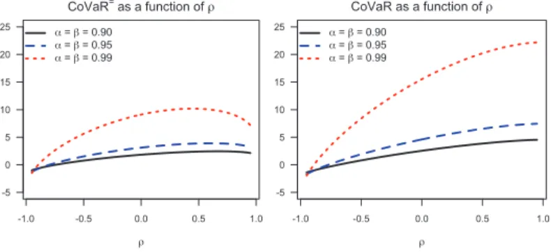
-1.0 -0.5 0.0 0.5 1.0 -1 0 1 2 3 4 5 CoVaR= _{as a function of} = = 0.90 = = 0.95 = = 0.99 -1.0 -0.5 0.0 0.5 1.0 -1 0 1 2 3 4 5 CoVaR as a function of = = 0.90 = = 0.95 = = 0.99 Fig. 4.1: CoVaR=

𝛼(𝑌|𝑋) and CoVaR𝛼(𝑌|𝑋) (i.e., with 𝛽 = 𝛼) in the bivariate normal model as

functions of 𝜌.

pronounced. In the special case𝛼 = 𝛽, the critical threshold𝜌₀is always equal to

1/√2.

A graphic illustration to this fact is given in Figure 4.1, showing

CoVaR=_𝛼(𝑌|𝑋) and CoVaR_𝛼(𝑌|𝑋) for 𝜌 ∈ [−1, 1] and𝛼 = 𝛽assuming values

0.90, 0.95, or0.99. The short writingCoVaR=_𝛼 refers toCoVaR=_𝛼,𝛼; analogously,

CoVaR_𝛼denotesCoVaR_𝛼,𝛼. This notation was used in the original definitions of

CoVaR=andCoVaR, which were restricted to𝛼 = 𝛽(cf. Remark2.3(b)). For the sake of simplicity we set𝜇_𝑌= 0and𝜎_𝑌= 1. These parameters have no influence on the decreasing or increasing behaviour ofCoVaRorCoVaR= as functions of𝜌.

Normalized values of CoVaR and CoVaR=

The relative impact of a stress event for𝑋 on the institution𝑌 can be quan-tified by the ratio CoVaR=_𝛼,𝛽(𝑌|𝑋)/ VaR_𝛼(𝑌) or byCoVaR_𝛼,𝛽(𝑌|𝑋)/ VaR_𝛼(𝑌). A similar indicator of systemic risk was proposed inAdrian and Brunnermeier

(2008). Figure4.2 shows these ratios for 𝛼 = 𝛽and 𝜇 = 0as functions of 𝛼. The different line types in the plots correspond to𝜌 = 0.5,0.7, and0.9. The ra-tiosCoVaR_𝛼=(𝑌|𝑋)/ VaR_𝛼(𝑌)are constant, which is also easy to see from (4.2). The interesting part here is the ordering of the lines for different𝜌. In case ofCoVaR=, the line for 𝜌 = 0.7 is above the two others, illustrating that the inconsistency problem persists for all confidence levels 𝛼 ∈ (1/2, 1). The plot ofCoVaR_𝛼(𝑌|𝑋)/ VaR_𝛼(𝑌) shows correct ordering for all𝛼 w.r.t. 𝜌, as guar-anteed by Theorem 3.6(a). Another observation one can make here is that

CoVaR_𝛼(𝑌|𝑋)/ VaR_𝛼(𝑌)is decreasing in𝛼. This, however, is a model property that seems to be related to the light tail of the normal distribution. In heavy-tailed models considered in Sections4.2and4.3the ratioCoVaR_𝛼(𝑌|𝑋)/ VaR_𝛼(𝑌)is increasing in𝛼.

0.90 0.92 0.94 0.96 0.98 1.00 1.2 1.4 1.6 1.8 2.0

Ratio CoVaR=/VaR as a function of and

0.5 0.7 0.9 0.90 0.92 0.94 0.96 0.98 1.00 1.2 1.4 1.6 1.8 2.0

Ratio CoVaR/VaR as a function of and 0.5 0.7 0.9

Fig. 4.2: Bivariate normal model with 𝜇𝑌= 0: Ordering of the ratios CoVaR=𝛼(𝑌|𝑋)/ VaR𝛼(𝑌) and

CoVaR𝛼(𝑌|𝑋)/ VaR𝛼(𝑌) for different 𝛼.

Backtesting and violation rates

The results above show thatCoVaRreflects the dependence between𝑋and𝑌

much more consistently than CoVaR=. An intuitive and very general explana-tion of this fact is that condiexplana-tioning on𝑋 ≥ VaR_𝛼(𝑋)corresponds to a reasonable “what if” question, whereas conditioning on𝑋 = VaR_𝛼(𝑋)does not. Indeed, the scenario{𝑋 ≥ VaR_𝛼(𝑋)}includes all possible outcomes for𝑋if𝑋is stressed, whereas the scenario{𝑋 = VaR_𝛼(𝑋)}selects only the most benign among them, thereby constituting an overly optimistic stress scenario.

In backtesting ofVaRone expects that𝑋exceedsVaR_𝛼(𝑋)with probabil-ity not larger than1 − 𝛼. Abbreviating “ConditionalVaR”, the term CoVaR=_𝛼,𝛽

suggests that 𝑌exceedsCoVaR_𝛼,𝛽= (𝑌|𝑋)with conditional probability1 − 𝛽or less, given that𝑋is stressed. The definition ofCoVaRunderstands stress of𝑋as

{𝑋 ≥ VaR_𝛼(𝑋)}, so that the expected violation rate forCoVaR_𝛼,𝛽under this stress scenario is by construction equal to1 − 𝛽. In contrast to that,CoVaR=is designed to have the violation rate1−𝛽under the less natural and more optimistic scenario

{𝑋 = VaR_𝛼(𝑋)}. As a consequence, the violation rates forCoVaR_𝛼,𝛽= backtesting experiments based on the natural stress scenario{𝑋 ≥ VaR_𝛼(𝑋)}are significantly higher than1 − 𝛽.

This issue is illustrated in Table4.1. The underlying Monte Carlo experiment generates an i.i.d. sample(𝑋_𝑖, 𝑌_𝑖) ∼N(0, 𝛴)for𝑖 = 1, . . . , 𝑛and counts the joint exceedances{𝑌_𝑖≥ CoVaR_𝛼,𝛽= (𝑌|𝑋), 𝑋_𝑖≥ VaR_𝛼(𝑋)}. TheCoVaR= violation rate for the stress scenario{𝑋 ≥ VaR_𝛼(𝑋)}is the ratio of the joint excess count and the count of the excesses{𝑋_𝑖≥ VaR_𝛼(𝑋)}. The violation rate forCoVaRis obtained analogously from the number of joint exceedances {𝑌_𝑖≥ CoVaR_𝛼,𝛽(𝑌|𝑋), 𝑋_𝑖≥ VaR_𝛼(𝑋)}. We chose𝑛 = 107and𝛼, 𝛽being either0.95or0.99.

It is remarkable that the violation rate forCoVaR= increases with 𝜌. This demonstrates that the underestimation of risk byCoVaR= is most pronounced

Table 4.1: Violation rates in the bivariate normal case. Monte Carlo backtesting with 𝑛 = 107and 𝛼, 𝛽 ∈ {0.95, 0.99}. Bound _{𝜌 = 0 𝜌 = 0.2 𝜌 = 0.5 𝜌 = 0.7 𝜌 = 0.9} CoVaR=0.95,0.95(𝑌|𝑋) 0.0503 0.0601 0.0857 0.1229 0.2520 CoVaR=0.99,0.99(𝑌|𝑋) 0.0099 0.0124 0.0189 0.0292 0.0875 CoVaR=0.95,0,99(𝑌|𝑋) 0.0101 0.0130 0.0213 0.0375 0.1224 CoVaR=0.99,0.95(𝑌|𝑋) 0.0500 0.0588 0.0785 0.1045 0.2053 CoVaR0.95,0.95(𝑌|𝑋) 0.0503 0.0500 0.0503 0.0495 0.0499 CoVaR0.99,0.99(𝑌|𝑋) 0.0099 0.0101 0.0104 0.0099 0.0098 CoVaR0.95,0.99(𝑌|𝑋) 0.0101 0.0102 0.0102 0.0099 0.0098 CoVaR0.99,0.95(𝑌|𝑋) 0.0500 0.0507 0.0509 0.0501 0.0491 -6 -4 -2 0 2 4 6 -6 -4 -2 0 24 6

Bivariate Normal for = 0.2

VaR0.95 CoVaR0.95= CoVaR0.95 -6 -4 -2 0 2 4 6 -6 -4 -2 0 246

Bivariate Normal for = 0.7

VaR0.95 CoVaR0.95= CoVaR0.95 -6 -4 -2 0 2 4 6 -6 -4 -2 0 246

Bivariate Normal for = 0.9

VaR0.95 CoVaR0.95= CoVaR0.95

Fig. 4.3: Bivariate normal samples (size 𝑛 = 2000) and the joint excess regions in the

backtesting experiment for 𝛼 = 𝛽 = 0.95.

in case of strong dependence and, hence, high systemic risk. At a high confi-dence level of𝛼 = 0.99and a strong correlations of𝜌 = 0.9, theCoVaR=_0.99,0.99and

CoVaR=_0.95,0.99levels are exceeded by up to 12 times as often as their nomenclature might suggest.

A graphical illustration of this issue is given in Figure4.3by bivariate normal samples from the simulation study described above. The horizontal lines mark the levels ofCoVaR=_𝛼(𝑌|𝑋)andCoVaR_𝛼(𝑌|𝑋), andVaR_𝛼(𝑌). The vertical lines markVaR_𝛼(𝑋). The joint excess counts are the numbers of points above the corre-sponding horizontal line and on the right hand side from the vertical line marking

VaR_𝛼(𝑋). The sample size is𝑛 = 2000, which suffices to demonstrate how corre-lation changes the shape of the sample cloud and thus increases the number of the joint excesses{𝑌_𝑖≥ CoVaR_𝛼=(𝑌|𝑋), 𝑋_𝑖≥ VaR_𝛼(𝑋)}.

Risk contribution measuresΔ

CoVaR

CoVaR

As mentioned in Section2,Adrian and Brunnermeier(2008) aims not atCoVaR=

itself, but at the difference betweenCoVaR= and some characteristic of an un-stressed state. The two most common definitions of such a risk contribution mea-sure areΔCoVaR=andΔmedCoVaR=(see (2.3) and (2.4)). In the bivariate normal case one hasVaR_𝛽(𝑌) = 𝜇_𝑌+ 𝜎_𝑌Φ−1(𝛽), so that (4.2) yields

ΔCoVaR=_𝛼,𝛽(𝑌) = 𝜎_𝑌(Φ−1(𝛼)𝜌 + Φ−1(𝛽) (√1 − 𝜌2_{− 1)) .}

For𝛼 = 𝛽this simplifies toΔCoVaR=_𝛼(𝑌) = 𝜎_𝑌Φ−1(𝛼) (𝜌 + √1 − 𝜌2_{− 1).} Regard-less of𝛼and𝛽,ΔCoVaR=inherits the non-monotonicity in𝜌fromCoVaR=. An illustration of this issue is given in Figure4.4, which shows plots ofΔCoVaR=and

ΔmedCoVaR=as functions of𝜌for𝛼 = 𝛽.

At a first glance,ΔmedCoVaR=seems to be an improvement because it is in-creasing in𝜌. In fact,ΔmedCoVaR=is even linear here. Due tomed(𝑋) = 𝜇_𝑋, (4.1) yields𝐹_{𝑌|𝑋=med(𝑋)}← (𝛽) = 𝜇_𝑌+ 𝜎_𝑌√1 − 𝜌2_Φ−1_{(𝛽). Applying (4.2), one obtains that}

ΔmedCoVaR_𝛼,𝛽= (𝑌)

= 𝜇_𝑌+ 𝜎_𝑌(Φ−1(𝛼)𝜌 + Φ−1(𝛽)√1 − 𝜌2_{) − (𝜇}

𝑌+ 𝜎𝑌Φ

−1_{(𝛽)√1 − 𝜌2)}

= 𝜎_𝑌Φ−1(𝛼)𝜌. (4.6)

Thus, in the bivariate normal model,ΔmedCoVaR=_𝛼,𝛽(𝑌|𝑋)is linear with positive slope that depends on𝜌and𝛼, but not on𝛽, i.e. precisely the confidence level for𝑌. In view of the linear structure (4.1) of the bivariate Gaussian model, this even appears reasonable. However, examples in Sections4.2and4.3show that

ΔmedCoVaR= is not a monotonic function of dependence parameters in other models. Thus the applicability ofΔmedCoVaR=is restricted to linear models of

-1.0 -0.5 0.0 0.5 1.0 -3 -2 -1 0 1 2 CoVaR as a function of = = 0.90 = = 0.95 = = 0.99 -1.0 -0.5 0.0 0.5 1.0 -3 -2 -1 0 1 2

med_{CoVaR as a function of}

= 0.90 = 0.95 = 0.99

Fig. 4.4: ΔCoVaR=

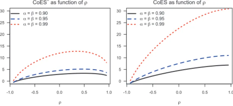
-1.0 -0.5 0.0 0.5 1.0 -2 0 2 4 6 CoES= as function of = = 0.90 = = 0.95 = = 0.99 -1.0 -0.5 0.0 0.5 1.0 -2 0 2 4 6 CoES as function of = = 0.90 = = 0.95 = = 0.99 Fig. 4.5: CoES=

𝛼(𝑌|𝑋) and CoES𝛼(𝑌|𝑋) in the bivariate normal model as functions of 𝜌.

type (4.1), where it is superfluous because it carries quite the same information as the correlation parameter𝜌or the linear regression parameter from the classical Capital Asset Pricing Model (the so-called CAPM-𝛽), which is equal to𝜌𝜎_𝑌/𝜎_𝑋in the present setting.

Extension from CoVaR to CoES

Due to Corollary3.10(a) we already know thatCoES_𝛼,𝛽is increasing in𝜌for all

𝛼and𝛽. The special case𝛼 = 𝛽is illustrated in Figure4.5, which also shows thatCoES= is not increasing in𝜌. Due to the light tail of the normal distribu-tion, these plots are similar to those ofCoVaRandCoVaR=in Figure4.1. A closer look at (2.2) confirms that the non-monotonicity ofCoES=in𝜌is inherited from

CoVaR=. Hence, also the best possible extension to Conditional Expected Short-fall based onCoVaR=fails to reflect dependence properly.

4.2 Bivariate

𝑡 distribution

The next example we consider is the bivariate𝑡distribution, which is elliptical, but heavy-tailed. The comparison follows the same scheme as in the previous sec-tion. A bivariate𝑡distributed random vector with𝜈 > 0degrees of freedom (bivari-ate𝑡(𝜈)) can be obtained as follows:

(𝑋, 𝑌) := (𝜇_𝑋, 𝜇_𝑌) + √𝜈

𝑊(̃𝑋, ̃𝑌) ,

where( ̃𝑋, ̃𝑌) ∼N(0, 𝛴)and𝑊 ∼ 𝜒2(𝜈), independent of( ̃𝑋, ̃𝑌). The parameters

𝜇_𝑋, 𝜇_𝑌∈ ℝspecify the location of(𝑋, 𝑌). For simplicity, we consider a centred model with𝜇_𝑋= 𝜇_𝑌 = 0.

It is well known that the bivariate𝑡distribution is elliptical with ellipticity ma-trix𝛴. The corresponding sample clouds have an elliptical shape (cf. Figure4.8).

-1.0 -0.5 0.0 0.5 1.0 -5 0 5 10 15 20 25 CoVaR= _{as a function of} = = 0.90 = = 0.95 = = 0.99 -1.0 -0.5 0.0 0.5 1.0 -5 0 5 10 15 20 25 CoVaR as a function of = = 0.90 = = 0.95 = = 0.99

Fig. 4.6: Bivariate 𝑡(3) distribution: CoVaR=

𝛼and CoVaR𝛼as functions of the correlation

parameter 𝜌.

The second moments of𝑋and𝑌are finite for𝜈 > 2, and in this case the correla-tion between𝑋and𝑌is equal to𝜌. The role of𝜌is the same as for all elliptical models: larger values of𝜌increase association between large values of𝑋and𝑌. Analytic expressions forCoVaR=orCoVaRare not obtainable in this model, so that computations have to be carried out numerically.

Monotonicity in𝜌

The behaviour ofCoVaR= andCoVaRas functions of the correlation parame-ter𝜌is shown in Figure4.6for𝜈 = 3. Similarly to the Gaussian case,CoVaRis increasing in𝜌due to Theorem3.6(a), whereasCoVaR=is not. Moreover, the rel-ative distance betweenCoVaR=andCoVaR(as it could be quantified by the ratio

CoVaR / CoVaR=) is larger than in the Gaussian case. A possible explanation to this effect could be the heavy tail of the𝑡(3)distribution.

0.90 0.92 0.94 0.96 0.98 1.00 1.0 1.5 2.0 2.5 3.0 3.5 4.0

Ratio CoVaR=_{/VaR as a function of and}

0.5 0.7 0.9 0.90 0.92 0.94 0.96 0.98 1.00 1.0 1.5 2.0 2.5 3.0 3.5 4.0

Ratio CoVaR/VaR as a function of and 0.5

0.7 0.9

Fig. 4.7: Bivariate 𝑡(3) distribution with 𝜇𝑌= 0: Ordering of the ratios CoVaR=𝛼(𝑌|𝑋)/ VaR𝛼(𝑌)

Normalized values of CoVaR and CoVaR=

Figure 4.7 shows the ratios CoVaR=_𝛼(𝑌|𝑋)/ VaR_𝛼(𝑌) and CoVaR_𝛼(𝑌|𝑋) / VaR_𝛼(𝑋)as functions of 𝛼for selected values of𝜌. This comparison is anal-ogous to Figure4.2 in the Gaussian case. Similarly to the Gaussian case, the ordering of CoVaR_𝛼=/ VaR_𝛼 with respect to the dependence parameter 𝜌 is inconsistent, whereas the ratiosCoVaR_𝛼/ VaR_𝛼are ordered correctly for all𝛼: the line for the largest𝜌is entirely above the line for the second largest𝜌, etc. In contrast to the Gaussian case, these ratios are increasing in𝛼. This could be explained by the heavy tail of the𝑡(3) distribution or by the positive tail dependence in the bivariate𝑡model.

Backtesting and violation rates

The backtesting study was implemented analogously to the bivariate Gaussian example. The results are shown in Table4.2, and they go in line with those from the Gaussian case. WhileCoVaR– again, by construction – has a violation rate close to1−𝛽, the violation rates ofCoVaR=are significantly higher and increasing in𝜌. Going up to36%for𝜌 = 0.9, the violation rates forCoVaR=are even higher than in the Gaussian model.

The corresponding sample plots with lines marking VaR_𝛼(𝑋),

CoVaR=_𝛼(𝑌|𝑋), and CoVaR_𝛼(𝑌|𝑋) are shown in Figure 4.8. Similarly to Fig-ure4.3, these graphics demonstrate how the increasing dependence parameter𝜌

changes the shape of the corresponding sample clouds and thereby increases the numbers of joint excesses.

Risk contribution measuresΔCoVaR=andΔmedCoVaR=

The comparison ofΔCoVaR=andΔmedCoVaR=is shown in Figure4.9. The graph-ics demonstrate clearly how theseCoVaR=based risk contribution measures

in-Table 4.2: Violation rates in the bivariate 𝑡(3) case. Monte Carlo backtesting with 𝑛 = 107_and

𝛼, 𝛽 ∈ {0.95, 0.99}. 𝜌 = 0 𝜌 = 0.2 𝜌 = 0.5 𝜌 = 0.7 𝜌 = 0.9 CoVaR=0.95,0.95(𝑌|𝑋) 0.1017 0.1213 0.1659 0.2202 0.3638 CoVaR=0.99,0.99(𝑌|𝑋) 0.0358 0.0433 0.0643 0.0939 0.1909 CoVaR=0.95,0.99(𝑌|𝑋) 0.0341 0.0429 0.0640 0.0944 0.1954 CoVaR=0.99,0.95(𝑌|𝑋) 0.1036 0.1229 0.1658 0.2184 0.3546 CoVaR0.95,0.95(𝑌|𝑋) 0.0497 0.0500 0.0499 0.0506 0.0504 CoVaR0.99,0.99(𝑌|𝑋) 0.0103 0.0099 0.0104 0.0105 0.0103 CoVaR0.95,0.99(𝑌|𝑋) 0.0100 0.0099 0.0100 0.0102 0.0101 CoVaR0.99,0.95(𝑌|𝑋) 0.0501 0.0493 0.0499 0.0508 0.0507

-10 -5 0 5 10

-10

-5

05

1

0 Bivariate Student-t(3) for = 0.2

VaR0.95 CoVaR0.95= CoVaR0.95 -10 -5 0 5 10 -10 -5 0 5 1

0 Bivariate Student-t(3) for = 0.7

VaR0.95 CoVaR0.95= CoVaR0.95 -10 -5 0 5 10 -10 -5 0 5 10

Bivariate Student-t(3) for = 0.9

VaR0.95 CoVaR0.95= CoVaR0.95

Fig. 4.8: Bivariate 𝑡(3) samples (size 𝑛 = 2000) and the joint excess regions in the backtesting

experiment for 𝛼 = 𝛽 = 0.95. -1.0 -0.5 0.0 0.5 1.0 -4 -2 0 2 4 6 8 10 CoVaR as a function of = = 0.90 = = 0.95 = = 0.99 -1.0 -0.5 0.0 0.5 1.0 -4 -2 0 2 4 6 8 10

med_{CoVaR as a function of}

= = 0.90 = = 0.95 = = 0.99

Fig. 4.9: ΔCoVaR=

𝛼and ΔmedCoVaR=𝛼as functions of 𝜌 in the bivariate 𝑡(3) model.

herit the inconsistency ofCoVaR=. BothΔCoVaR= andΔmedCoVaR=fail to be increasing with respect to the dependence parameter𝜌, and the shapes of the corresponding curves are similar to those of CoVaR= in Figure 4.6. Although

ΔmedCoVaR=is slightly better behaved thanΔCoVaR=, it is still strongly incon-sistent with respect to𝜌. In particular, this example demonstrates that the mono-tonicity ofΔmedCoVaR=with respect to𝜌in the Gaussian case is a special prop-erty of the bivariate Gaussian model, so that the advantage ofΔmedCoVaR=over

ΔCoVaR=is rather limited in this respect.

Extension from CoVaR to CoES

The comparison ofCoESvs.CoES= is shown in Figure4.10. The monotonicity or non-monotonicity in𝜌is again inherited fromCoVaRorCoVaR=respectively. See also Corollary3.10(a).

-1.0 -0.5 0.0 0.5 1.0 0 5 10 15 20 25 30 CoES= _{as function of} = = 0.90 = = 0.95 = = 0.99 -1.0 -0.5 0.0 0.5 1.0 0 5 10 15 20 25 30 CoES as function of = = 0.90 = = 0.95 = = 0.99 Fig. 4.10: CoES=

𝛼(𝑌|𝑋) and CoES𝛼(𝑌|𝑋) in the bivariate 𝑡(3) model as functions of 𝜌.

1 2 3 4 5 6 0 5 10 15 20 25 30 CoVaR= _{as function of} = = 0.90 = = 0.95 = = 0.99 1 2 3 4 5 6 0 5 10 15 20 25 30 CoVaR as a function of = = 0.90 = = 0.95 = = 0.99

Fig. 4.11: Gumbel copula with 𝑡(3) margins: CoVaR=

𝛼(𝑌|𝑋) and CoVaR𝛼(𝑌|𝑋) as functions of 𝜃.

4.3 Gumbel copula with

𝑡 margins

The last model we consider is obtained by endowing a bivariate Gumbel copula (cf. (3.6)) with𝑡margins. Thus it has the same heavy-tailed margins as the previous example, but a different dependence structure. Indeed, being an extreme value copula, it allows in particular more generously for joint excesses. An illustration of the sample clouds generated from this distribution is given in Figure4.13.

On the qualitative level, all comparison results obtained in this case are sim-ilar to the bivariate𝑡model, so that a brief overview is fully sufficient:

– Corollary3.8guarantees thatCoVaR_𝛼,𝛽is increasing with respect to the de-pendence parameter𝜃, whereasCoVaR=_𝛼,𝛽fails to be increasing when depen-dence is at its largest (see Figure4.11for the case𝛼 = 𝛽). The strongest decay ofCoVaR=takes place for𝜃 ∈ (1.5, 2)and slows down for𝜃 > 2. On the other hand,CoVaR_𝛼is almost constant for𝜃 > 2. It seems that for𝜃 > 2the joint distribution of large values of(𝑋, 𝑌)is almost comonotonic, so that there is no much change after𝜃exceeds2.

0.90 0.92 0.94 0.96 0.98 1.00 1 2 3 4 5 6 7

Ratio CoVaR=_{/VaR as a function of}

1.1 1.4 3 0.90 0.92 0.94 0.96 0.98 1.00 1 2 3 4 5 6 7

Ratio CoVaR/VaR as a function of 1.1

1.4 3

Fig. 4.12: Gumbel copula with 𝑡(3) margins: Ordering of the ratios CoVaR=

𝛼(𝑌|𝑋)/ VaR𝛼(𝑌) and

CoVaR𝛼(𝑌|𝑋)/ VaR𝛼(𝑌) for different 𝛼.

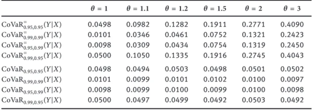
Table 4.3: Violation rates for the Gumbel copula with 𝑡(3) margins: Monte Carlo backtesting

with 𝑛 = 107_{and 𝛼, 𝛽 ∈ {0.95, 0.99}.} 𝜃 = 1 𝜃 = 1.1 𝜃 = 1.2 𝜃 = 1.5 𝜃 = 2 𝜃 = 3 CoVaR=0.95,0.95(𝑌|𝑋) 0.0498 0.0982 0.1282 0.1911 0.2771 0.4090 CoVaR= 0.99,0.99(𝑌|𝑋) 0.0101 0.0346 0.0461 0.0752 0.1321 0.2423 CoVaR=0.95,0.99(𝑌|𝑋) 0.0098 0.0309 0.0434 0.0754 0.1319 0.2450 CoVaR= 0.99,0.95(𝑌|𝑋) 0.0500 0.1050 0.1335 0.1916 0.2745 0.4043 CoVaR0.95,0.95(𝑌|𝑋) 0.0498 0.0494 0.0503 0.0498 0.0501 0.0502 CoVaR0.99,0.99(𝑌|𝑋) 0.0101 0.0099 0.0101 0.0102 0.0100 0.0097 CoVaR0.95,0.99(𝑌|𝑋) 0.0098 0.0099 0.0100 0.0099 0.0100 0.0098 CoVaR0.99,0.95(𝑌|𝑋) 0.0500 0.0497 0.0499 0.0492 0.0503 0.0492 -15 -10 -5 0 5 10 15 -15 -10 -5 0 51 0 15 Gumbel/t(3) for = 1.1 VaR0.95 CoVaR0.95 = CoVaR0.95 -15 -10 -5 0 5 10 15 -15 -10 -5 0 51 0 1

5 _VaRGumbel/t(3) for = 1.4

0.95 CoVaR0.95 = CoVaR0.95 -15 -10 -5 0 5 10 15 -15 -10 -5 0 51 0 1

5 _VaRGumbel/t(3) for = 3

0.95 CoVaR0.95

= CoVaR0.95

Fig. 4.13: Gumbel copula with 𝑡(3) margins: simulated samples (size 𝑛 = 2000) and the joint

1 2 3 4 5 6 0 2 4 6 8 10 CoVaR as a function of = = 0.90 = = 0.95 = = 0.99 1 2 3 4 5 6 0 2 4 6 8 10 med CoVaR as a function of = = 0.90 = = 0.95 = = 0.99

Fig. 4.14: Gumbel copula with 𝑡(3) margins: ΔCoVaR=

𝛼and ΔmedCoVaR=𝛼as functions of 𝜃.

1 2 3 4 5 6 0 10 20 30 40 CoES= as function of = = 0.90 = = 0.95 = = 0.99 1 2 3 4 5 6 0 10 20 30 40 CoES as function of = = 0.90 = = 0.95 = = 0.99

Fig. 4.15: Gumbel copula with 𝑡(3) margins: CoES=

𝛼(𝑌|𝑋) and CoES𝛼(𝑌|𝑋) as functions of 𝜃.

– The ratiosCoVaR_𝛼(𝑌|𝑋)/ VaR_𝛼(𝑌)are ordered correctly with respect to𝜃, whereas the ratiosCoVaR=_𝛼(𝑌|𝑋)/ VaR_𝛼(𝑌)are not (see Figure4.12). – The violation rates forCoVaR_𝛼,𝛽= in a simulated backtesting study are

signif-icantly larger than1 − 𝛽, going up to40%for𝛼 = 𝛽 = 0.95and𝜃 = 3(cf. Table4.3and Figure4.13). This is even more than in the bivariate𝑡case. – BothΔCoVaR=andΔmedCoVaR=fail to be increasing in𝜃(Figure4.14). – Again,CoESis increasing in𝜃whileCoES=is not; see Corollary3.10(a) and

Figure4.15.

5 Conclusions

The present paper demonstrates that the alternative definition of Conditional Value-at-Risk proposed inGirardi and Ergün(2013), Klyman(2011) (hereCoVaR)

gives a much more consistent response to dependence than the original definition used inAdrian and Brunnermeier(2008,2009,2010) (hereCoVaR=).

The general results in Section 3 show that the monotonicity of

CoVaR_𝛼,𝛽(𝑌|𝑋) with respect to dependence parameters is related to the concordance ordering of bivariate distributions or copulas. This gives the notion of CoVaR based on the stress scenario {𝑋 ≥ VaR_𝛼(𝑋)} a solid mathematical fundament. On the other hand, comparative studies in Section 4 show that conditioning on {𝑋 = VaR_𝛼(𝑋)} makesCoVaR= and its derivatives unable to detect systemic risk where it is most pronounced. Related counterexamples include several popular models, in particular the very basic bivariate normal case.

Based on these results, we claim that, if Conditional Value-at-Risk of an insti-tution (or system)𝑌related to a stress scenario for another institution𝑋should enter financial regulation, then it should use conditioning on{𝑋 ≥ VaR_𝛼(𝑋)}. This kind of stress scenario has a much more meaningful practical interpretation than the highly selective and over-optimistic scenario{𝑋 = VaR_𝛼(𝑋)}. Condition-ing on{𝑋 ≥ VaR_𝛼(𝑋)}also makesCoVaRmore similar to the systemic risk mea-sures proposed inAcharya et al.(2010), Goodhart and Segoviano(2008), Huang et al.(2012), Zhou(2010).

The question how to define risk contribution measures based on stress events to the financial system is currently open. BesidesCoVaR,CoESwith proper con-ditioning may also be an option. The advantage ofCoESoverCoVaRis its co-herency. In the caseVaRvs.ES, this point has gained new interest from regulators, see e.g.Basel Committee on Banking Supervision(2012), Gauthier et al.(2012).

In some sense,CoVaR=repeats two times the design error that is responsible for the non-coherency ofVaR. In the first step, it follows theVaRparadigm and thus favours a single conditional quantile of𝑌over an average of such quantiles. In the second step, it favours the most benign outcome of𝑋in a state of stress over considering the full range of possible values in this case. Financial regula-tion based onCoVaR=has the potential to introduce additional instability, to set wrong incentives, and to create opportunities for regulatory arbitrage.

Another argument supportingCoESis that it is particularly suitable for stress testing. In a system with several factors𝑋₁, . . . , 𝑋_𝑑, the numbersCoES_𝛼

𝑖,𝛽(𝑌|𝑋𝑖)

describe the influence of the different𝑋_𝑖on𝑌. Assigning relative weights𝑤_𝑖to the scenarios𝑋_𝑖≥ VaR_𝛼

𝑖(𝑋𝑖)and taking the weighted sum

𝑑

∑

𝑖=1

𝑤_𝑖CoES_𝛼

𝑖,𝛽(𝑌|𝑋𝑖), (5.1)

one always obtains a sub-additive risk measure. If the weights𝑤_𝑖sum up to1, the resulting risk measure is coherent in the sense ofArtzner et al.(1999). The choice

of the weights𝑤_𝑖or of the confidence levels𝛼_𝑖may change over time, incorporat-ing the newest information about the health of the institutions𝑋₁, . . . , 𝑋_𝑑.

To make the weighted risk measure (5.1) even more meaningful, one could modify it by implementing not only the single risk factor excesses𝑋_𝑖≥ VaR_𝛼

𝑖(𝑋𝑖),

but also the joint ones. Consistent choice of the corresponding weights can be derived by methods presented inRebonato(2010). A detailed discussion of this goes beyond the scope of the present paper and would also require additional mathematical research.

Motivated by the recent financial crisis and the following discussions on ap-propriate reforms in financial regulation, systemic risk measurement has become a vivid topic in economics and econometrics. Our results show that some impor-tant contributions are also to be made in related mathematical fields, including probability and statistics. In particular, the dependence consistency or, say, de-pendence coherency of systemic risk indicators is a novel problem area that needs further study. The present paper provides first examples and counter-examples for compatibility of systemic risk indicators with the concordance order. The ques-tions for general characterizaques-tions or representaques-tions of functionals with this property are currently open.

In addition to dependence consistency, implementation of systemic risk mea-sures in practice obviously needs estimation methods. The estimation ofCoVaR

in GARCH models is discussed inGirardi and Ergün(2013). As non-parametric es-timation of rare events requires a lot of data, methods from Extreme Value Theory may be used to extrapolate the rear events from a larger number of data points. Recent applications of these methods to the estimation of systemic risk from mar-ket data includeZhou(2010) andNguyen and Samorodnitsky(2013). Another ap-proach to the estimation of systemic risk levels via a so-called herd behaviour in-dex (HIX) is taken inDhaene et al.(2012). Using instantaneous market data, this method has the potential to react immediately when new information enters the financial markets.

We would like to conclude with a comment on the applicability ofCoVaR. A lot of market data based stress measures failed to pick up the subliminal build-up of systemic risk in the run-build-up to the financial crisis. Since CoVaR estimates are based on market data, they can only reflect the information that is already available in the financial markets. In particular, mutual exposures of financial in-stitutions are highly relevant to the stability of financial systems, but for obvious reasons most of this information is not disclosed. Using a unique dataset, this approach is pursued inCont et al.(2013), where interbank exposure data – repre-senting potential future losses – is used to measure systemic risk. Therefore, we consider CoVaR rather as an indicator of current “market temperature” than as a genuine early warning measure. However, as our results illustrate, consistent

quantification of market stress is highly important. It is particularly relevant to regulators when evaluating different policy responses to stressed financial mar-kets.

Acknowledgement: The authors would like to thank Paul Embrechts for

sev-eral fruitful discussions related to this paper. Georg Mainik thanks RiskLab, ETH Zurich, for financial support.

Received April 10, 2013; accepted July 11, 2013.

References

Acharya, V. V., L. H. Pedersen, T. Philippon, and M. Richardson (2010). Measuring systemic risk. Preprint,http://papers.ssrn.com/abstract_id=1573171.

Adrian, T. and M. Brunnermeier (2008). Covar. Preprint,http://citeseerx.ist.psu.edu/viewdoc/ download?doi=10.1.1.140.7052&rep=rep1&type=pdf.

Adrian, T. and M. Brunnermeier (2009). Covar. Preprint,http://papers.ssrn.com/sol3/papers. cfm?abstract_id=1269446.

Adrian, T. and M. Brunnermeier (2010). Covar. Preprint,http://www.princeton.edu/~markus/ research/papers/CoVaR.

Artzner, P., F. Delbaen, J.-M. Eber, and D. Heath (1999). Coherent measures of risk. Math.

Fi-nance 9(3), 203–228.

Balkema, G. and P. Embrechts (2007). High Risk Scenarios and Extremes. Zurich Lectures in Advanced Mathematics. European Mathematical Society (EMS), Zürich.

Basel Committee on Banking Supervision (2012, May). Fundamental review of the trading book. Consultative document, Bank for International Settlements (BIS).

Bisias, D., M. Brunnermeier, A. W. Lo, and S. Valavanis (2012). A survey of systemic risk analyt-ics. Technical report, U.S. Department of Treasury, Office for Financial Research. Boss, M., H. Elsinger, M. Summer, and S. Thurner 4 (2004). Network topology of the interbank

market. Quantitative Finance 4(6), 677–684.

Cambanis, S. and G. Simons (1982). Probability and expectation inequalities. Probability

The-ory and Related Fields 59, 1–25.

Choi, Y. and R. Douady (2012). Financial crisis dynamics: attempt to define a market instability indicator. Quantitative Finance 12(9), 1351–1365.

Cont, R., A. Moussa, and E. B. Santos (2013). Network structure and systemic risk in banking systems. In J. Fouque and J. Langsam (Eds.), Handbook on Systemic Risk, pp. 327–368. Cambridge University Press.

Dhaene, J. M. L., D. Linders, W. Schoutens, and D. Vyncke (2012). The herd behavior index: A new measure for the implied degree of co-movement in stock markets. Insurance:

Math-ematics and Economics 50(3), 357–370.

Embrechts, P. and M. Hofert (2010). A note on generalized inverses. Math. Meth. Oper. Res. 77, 423–432.