HAL Id: halshs-00717624
https://halshs.archives-ouvertes.fr/halshs-00717624
Submitted on 13 Jul 2012
HAL is a multi-disciplinary open access archive for the deposit and dissemination of sci-entific research documents, whether they are pub-lished or not. The documents may come from teaching and research institutions in France or abroad, or from public or private research centers.
L’archive ouverte pluridisciplinaire HAL, est destinée au dépôt et à la diffusion de documents scientifiques de niveau recherche, publiés ou non, émanant des établissements d’enseignement et de recherche français ou étrangers, des laboratoires publics ou privés.
Trade and productivity: self-selection or
learning-by-exporting in India
Jamal Ibrahim Haidar
To cite this version:
Jamal Ibrahim Haidar. Trade and productivity: self-selection or learning-by-exporting in India. 2012. �halshs-00717624�
Documents de Travail du
Centre d’Economie de la Sorbonne
Trade and productivity : Self-selection or learning-by-exporting in India
Jamal Ibrahim HAIDAR
TRADE AND PRODUCTIVITY: SELF-SELECTION OR
LEARNING-BY-EXPORTING IN INDIA
JAMAL IBRAHIM HAIDAR
1May 2012
1 The World Bank, Washington DC, United States; Paris School of Economics, Paris, France; and
University of Paris 1 Pantheon-Sorbonne, Paris, France. E-mail: [email protected]; [email protected]; and [email protected]. The author circulated the first draft of this paper in 2009. The author would like to thank Allen Dennis, Ibrahim Elbadawi, Caroline Freund, Karim Ismail, Aart Kraay, Mustapha Kamel Nabli, and three anonymous referees for helpful comments and discussions as well as DIMeco Ile-de-France for financial support. Mohammad Mahdi Saleh Sbeiti provided inspiration. The findings, interpretations, and conclusions expressed in this paper are entirely those of the author. They do not necessarily represent the views of the International Bank for Reconstruction and Development/World Bank and its affiliated organizations, or those of the Executive Directors of the World Bank or the governments they represent.
Abstract:
Recent literature tried to explain the Indian growth miracle in different ways, ranging from trade liberalization to industrial reforms. Using data on Indian manufacturing firms, this paper analyzes the relationship between firm's productivity and export market participation during 1991-2004. While it provides evidence of the self-selection hypothesis by showing that more productive firms become exporters, the results do not show that entry into export markets enhances productivity. The paper examines the explanation of self selection hypothesis for total factor productivity differences across 33,510 exporting and non-exporting firms. It uses propensity score matching to test the learning-by-exporting hypothesis. In line with the prediction of recent heterogeneous firm models of international trade, the main finding of the paper is: more productive firms become exporters but it is not the case that learning by exporting is a channel fuelling growth in Indian manufacturing.
La littérature récente a essayé par différentes manières d'expliquer la miracle de la croissance indienne, allant de la libéralisation des échanges aux réformes industrielles. En utilisant les données sur les entreprises manufacturières indiennes, cet article analyse la relation entre la production des entreprises et la participation du marché d'exportation entre 1991 et 2004. Tandis que les résultats fournissent des épreuves sur l'hypothèse de l'auto-sélection en montrant que les entreprises les plus productives deviennent des exportateurs, les résultats ne prouvent pas que l'entrée sur les marchés d'exportation augmente la productivité. L'article examine l'hypothèse de l'auto-sélection pour les différences du facteur total de productivité entre 33,510 entreprises exportatrices et non exportatrices. Il utilise le score de propension pour tester l'hypothèse d'apprentissage par l'exportation. Conformément avec la prédiction des modèles récents des entreprises hétérogènes du commerce international, la principale conclusion de l'article est la suivante: les entreprises les plus productives deviennent des exportateurs, mais ce n'est pas le cas que l'apprentissage par l'exportation est un canal alimentant la croissance dans le secteur manufacturier Indien.
JEL codes: C12, F10, F20, F40, L1, L2, and L6
Keywords: trade, learning-by-exporting hypothesis, self-selection hypothesis, total factor productivity, causality, heterogeneous firm model
I. Introduction
Exporters tend to outperform non-exporters. The direction of causality - productivity increases exports or exports enhances productivity – within this relationship is, however, still under discussion. Do more productive firms within an industry export? What are the determinants behind different trade patterns within an industry? How are these differences in trade behavior related to productivity differences among firms? This paper analyzes these questions empirically for a sample of firm data from the manufacturing industry in India, a country that has not yet been well investigated from this perspective.
There are two alternative, but not mutually exclusive, hypotheses on why exporters can be expected to be more productive than non-exporting firms (see Bernard and Wagner 1997; Bernard and Jensen 1999): self-selection or learning-by-exporting.
The first hypothesis points to self-selection (SS) of the more productive firms into export markets. The reason for this expectation is that there are additional costs of selling goods in foreign countries. The range of extra costs includes transportation costs, distribution or marketing costs, personnel with skills to manage foreign networks, or production costs in modifying current domestic products for foreign consumption. These costs provide an entry barrier that less successful firms cannot overcome. Firms face difficulties in foreign market, due to the existence of sunk costs associated with selling abroad and fiercer competition in international markets. For example, Roberts and Tybout (1997) and Bernard and Wagner (2001) find evidence for the existence of sunk costs in exporting.
In addition, competition could be fiercer outside home market, a feature that would again allow only the most productive firms to do well abroad. This explanation is
in line with the assumption made in the theoretical literature of international trade with heterogeneous firms that high-performing firms self-select themselves into foreign markets. Bernard and Jensen (1999) find that exporters have all their desirable characteristics before taking up exporting, and that the performance paths of exporters and non-exporters do not diverge following the launch of export activities by the former. Cross-section differences between exporters and non-exporters, therefore, may in part be explained by ex ante differences between firms: According to the SS hypothesis, in the period prior to their entry, the productivity distribution of entering exporters should dominate the productivity distribution of non-exporters.
The second hypothesis points to the role of learning-by-exporting. Knowledge flows from international buyers and competitors help to improve the post-entry performance of export starters. Furthermore, firms participating in international markets are exposed to more intense competition and must improve faster than firms who sell their products domestically only. Exporting makes firms more productive.
Empirical papers have investigated the role of exports in promoting growth in
general2, and productivity in particular, using aggregate data for countries and industries
for a long time. However, only recently have comprehensive longitudinal data at the firm level been used to look at the extent and causes of productivity differentials between exporters and their counterparts (which sell on the domestic market only).
For a decade following the seminal paper by Bernard and Jensen (1995), researchers all over the world used firm level data to investigate the relationship between exporting and productivity in micro-econometric studies. Wagner (2007) surveyed the
2 Another line of research - i.e. Amin and Haidar (2011), Haidar (2009), Haidar (2012) - looked at the impact of export facilitation and
empirical strategies applied, and the results produced, in micro-econometric studies published between 1995 and 2004. In general, he found that the more productive firms self-select into export markets, while exporting does not necessarily improve productivity. Among the countries covered are industrialized countries (e.g., U.S., UK, Canada, Germany); Latin American countries (Chile, Colombia, Mexico); Asian countries (China, Korea, Indonesia, Taiwan); transition countries (Estonia, Slovenia); and least developed countries from sub-Saharan Africa. In particular, these findings include ones for Chile between 1990 and 1996 in Alvarez and Lopez (2005); for China between 1988 and 1992 in Kraay (2002); for Colombia between 1981 and 1991, Mexico between 1986 and 1990, and Morocco between 1984 and 1991 in Clerides, Lach, and Tybout (1998); and for Indonesia between 1990 and 1996 in Blalock and Gertler (2004).
However, India has not been explored in this literature. Nevertheless, it seems important to study the Indian context for two reasons. First, India is a large developing country, so it is useful to understand Indian exporting patterns. Second, India’s growth in manufacturing and particularly in exporting has been slower than that of many other developing countries (notably China), so it is interesting to understand the drivers of Indian exports.
Hence, this paper adds to the empirical literature on the direction of causality between trade and firm productivity by studying a particularly important developing country, India. Using longitudinal micro data on Indian manufacturing firms – industry accounts for 54.6% of the GDP and employs 17% of the workforce - this paper examines the validity of self selection and learning-by-exporting hypotheses for total factor productivity differences across 33,510 exporting and non-exporting Indian manufacturing
firms between 1991 and 2004. While it provides evidence of the self-selection hypothesis by showing that more productive firms become exporters, the paper does not find that entry into export markets enhances productivity. The paper uses propensity score matching to test the learning-by-exporting hypothesis. Firms which face foreign competition perform better than their domestic competitors years before they enter export markets. The changes in characteristics of exporting firms before they start exporting are not statistically different than those of the firms that serve only the domestic markets. While there is weak evidence as to whether these exporting firms prepare themselves consciously for the international markets, the main result is robust.
The paper is organized as follows. Section II describes the data. Section III.A presents the export premium calculation methodology. Section III.B estimates total factor productivity. Sections III.C and III.D sketch the self selection hypotheses along with related empirical evidence as well as it applies propensity score matching to test the evidence for learning due to exposure to international markets. Section IV concludes.
II. Data
We use an Indian firm-level panel dataset of balance sheets and income statements spanning 14 years (1991-2004) throughout the analysis. The data comes from the Center for Monitoring the Indian Economy (CMIE) Prowess database. We limit the analysis to manufacturing firms because the main firm-level productivity measure used in the estimations is the total factor productivity (TFP), which is not an appropriate measure of productivity for non-manufacturing firms as these firms have a different structure of production than manufacturing ones. The dataset covers 33,510 domestically-owned
manufacturing companies categorized by sectors. The largest sectors, measured by the number of companies, are food products, textiles, chemicals, basic metals and machinery.
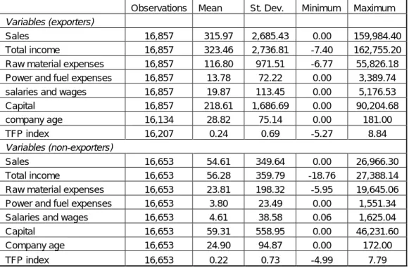
Table 1 provides descriptive statistics. The average percentage of exporters in total firms is 55 %. The firms that change their export status from non-export to export (entrant) and from export to non-export (quitter) constitute on average 5.5 % and 3.5 % of all firms, respectively across time. Exporting firms have on average larger sales, income and capital (Table 2). They spend more on raw materials, power and fuel expenses, and pay higher wages. Non-exporting firms tend to be younger than exporting firms. The TFP index is on average larger for exporters although the difference does not appear to be statistically significant.
However, the unbalanced nature of the sample, frequency of entry and exit behavior of firms, and missing observations make it difficult to interpret these results. A more formal and systematic analysis that takes into account the consistency of firms in terms of export behavior is required for a reliable comparison of exporters and non-exporters.
[Insert Table 1] [Insert Table 2]
III. Empirical model and analysis
The below four subsections provide estimation of export premium measurement and TFP as well as present empirical tests for the SS and LE hypothesis.
To document the differences between exporters and non-exporters, we measure the export premium (ceteris paribus percentage differences in firm characteristics between exporters and non-exporters) for each year during the 1991-2004 sample period. The main firm characteristics of interest are productivity measure (TFP), capital, sales, and unit labor cost, which is obtained by dividing total labor cost (salaries and wages) by the value of real output. Following Bernard and Jensen (1999), we estimate the export
premium for each firm i in each year by regressing the firm characteristics on an export
dummy and a set of control variables. More specifically, the export premia is estimated from a regression of the following form:
(1)
where represents the firm characteristics of interest (productivity measure –TFP,
capital, sales, and unit labor cost -salaries and wages/value of real output); is a
dummy for the current export status (1 if firm is an exporter, 0 otherwise);Industryi
dummy includes the 2-digit NIC codes ; and is a vector of firm-specific controls
(in logs except for size dummy), which include different combinations of firm
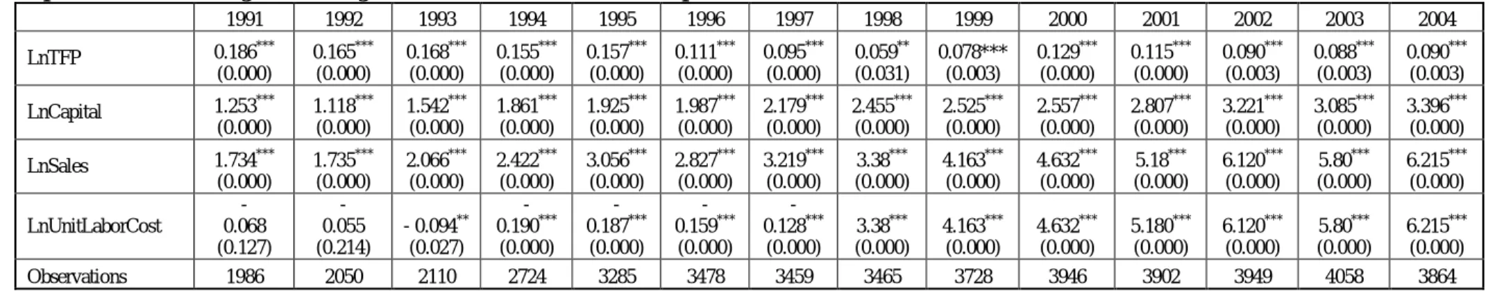
characteristics such as a firm size dummy, firm age and capital.3 . Table 3 presents the
results of the export premium regressions.
[Insert Table 3]
III.B Total Factor Productivity estimation
3 We classify each firm as large, medium or small in size, following Topalova (2004), depending on its average sales over the span of
the data. We include the firm in the “large size” category if average sales over the entire period are in the top 1 percent of the distribution; in the “medium size” category if sales are greater than the median, excluding the top 1 percentile of the distribution; or in the “small size” category if average sales over the period are less than the median. The standard measure in the literature for firm size is the employment level.
i i i
i
i Export Industry Control
X ln i X i Export i i Control
The ordinary least squares estimation of TFP - as the difference between actual and predicted output - leads to omitted variables bias since the firm’s choice of inputs is likely to be correlated with any unobserved firm-specific productivity shocks. Adding firm fixed effects into the estimation could solve the simultaneity problem if productivity is assumed to be time-invariant. However, this strategy is not appropriate since we are interested in changes in firm-level productivity.
The consistent firm-level measure of TFP, which we use in this paper, is constructed based on the methodology of Levinsohn and Petrin (2003). Assuming a Cobb Douglas production function, this methodology uses firm’s raw material inputs to correct for the simultaneity in the firm’s production function.
(2)
where y denotes output, l denotes labor, e denotes electricity consumption, m denotes
raw material inputs, k denotes capital, and w denotes the unobservable part of the
productivity shock that is correlated with the firm’s inputs. All variables are expressed in
natural logarithm.4 We rewrite (2) as:
(3)
where (ki,t,ei,t) is partially linear (linear in variable inputs and non-linear in electricity
and capital) as follows:
) , ( ) , (ki,t ei,t kki,t wi,t ki,t ei,t (4)
4 All variables that enter into TFP estimation are deflated using appropriate deflators from India’s National Account Statistics. Value
of output is deflated using the corresponding industry deflators. Energy and fuel expenses are deflated by a fuel and energy deflator. Salaries and wages as well as material expenses are deflated by the wholesale price index. Finally, gross fixed assets are converted to real terms by a capital goods deflator. Energy and fuel consumption is used as the intermediate input as a proxy for unobserved productivity shocks. t i t i t i k t i m t i p t i l t i l e m k w y, , , , , , , t i t i t i t i m t i l t i l m k e y, , , ( ,, ,),
We estimate equation (2) following the approach of Robinson (1988). The goal is
to obtain the estimates on the coefficients of inputs that enter (2) linearly (i.e. l,m).
Then, we define Vi,t yi,t lli,t mmi,t
and estimate the following equation:
t i t i t i k t t i k t i k g k e V, , (1 ,1), ,
(5)
where g(.) is a function of lagged values of and k . We approximated this function by
a high-order polynomial expression in t1 and kt1. We conducted the estimation using
2-digit National Industrial Classification codes (due to small number of companies in some of the 4-digit level industries) and over two time periods: a period of high-growth (before 1996) and a period of low-growth (after 1996). Having obtained consistent coefficients on the production inputs, we estimated the TFP using the initial production function.
Finally, after obtaining TFP measures, we created a TFP index in order to make
the estimated TFP comparable across industries.5 The resulting TFP index serves as the
dependent variable in all the regressions.
III.C Self-selection hypothesis
Exports and firm productivity can be linked via at least two different ways, as explained above. This subsection addresses the self-selection hypothesis: better firms are more likely to enter into export markets.
The scale of operations differs significantly between exporters and non-exporters. Exporters produce on average 3.75 times more than non-exporters. After controlling for
5
The productivity index is calculated as the logarithmic deviation of a firm in a particular industry from a reference firm’s productivity in that same industry in a base year. The productivity of the reference firms in each industry is calculated from the respective industry’s TFP regression, using the mean log output and mean log input level in 1988-89.
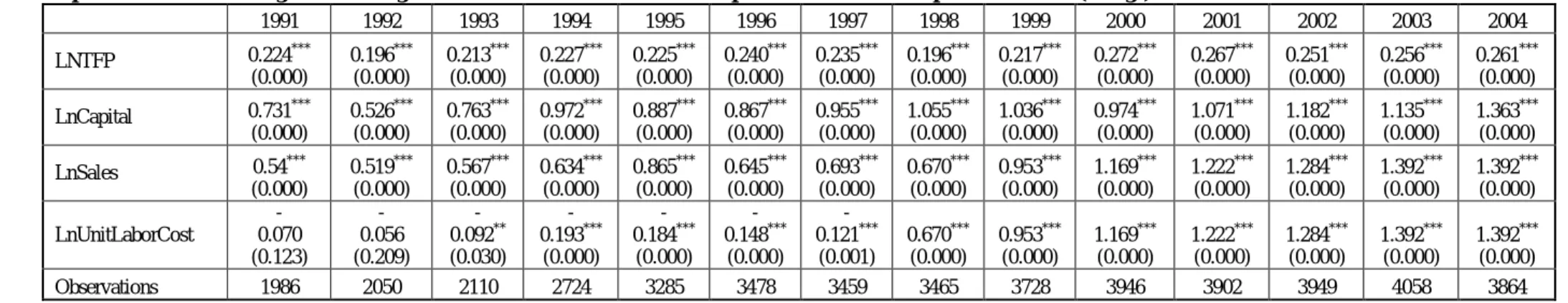
capital endowment, this average difference drops down to 9%. Moreover, exporters employ more capital and have lower unit labor cost than non-exporters. Even after controlling for firm size, exporters employ on average 97% more capital than non-exporters. The differences in sales and capital endowment become more noticeable after 1997. The average unit labor cost is 12.4 % lower for exporters. Controlling for capital endowment in addition to firm size leads to a slightly larger average gap (-13.4 %) for the unit labor cost, as shown in the average coefficients in Table 3 and Table 4. The statistical significance of the difference increases when capital is included in the controls. The regression results reported so far confirm the previous robust findings for other countries. Exporters have significantly different characteristics and exhibit superior performance in terms of productivity, sales, capital endowment and unit labor cost during each year in the sample.
The above cross-section analysis documents the different characteristics of exporters and non-exporters. However, this test is not sufficient to identify whether the firms with desirable characteristics self-select into export markets. To address this issue, we compare the performance of export-starters with non-exporters several years before entry.
Similar studies defined export-starters in different ways in the literature. An export-starter is defined in Bernard and Wagner (1997) as a plant that exports for the first time after at least three years in the sample. Accordingly, the subsample includes only plants that have at least four consecutive annual observations and do not export in any of their first three annual observations. Bernard and Jensen (1999) follow a similar approach. Serti and Tomasi (2008) define export-starters as firms that do not export at
least for two years and continue to export subsequent to their entry. Undoubtedly, these definitions above as well as others not mentioned here are influenced by data restrictions. The approach of Serti and Tomasi (2008) has the clear advantage of identifying continuous export behavior. Defining a firm as an export-starter based on whether the firm exports for the first time after a few years might be unsatisfactory in that the firm in question could stop exporting after one year or so. If the export behavior is not consistent and continuous over time for the export-starters, these firms would not be exposed to the benefits of participating in the international markets, if any, to a measurable extent. Thus, it would be problematic to draw a sound conclusion from this type of analysis.
[Insert Table 4]
Hence, we divide the sample into two sub-periods 1991-1997 and 1998-2004 in order to have consistent export behavior data and a reasonable number of observations in the analysis. The firms that do not export for the first three years in the sample, and export starting 1994 until 1997 are defined as the export starters for the first period. The firms that do not export for the first three years in the sample, and start export starting 2001 until 2004 are defined as the export starters for the second period. In each sample period, we define non-exporters as firms that did not export in any of the years in the selected sample periods. We follow the same regression in equation (1), but with different export status variable, to measure the systematic differences of plant characteristics between export-starters and non-exporters:
(6)
where is a dummy for the export-entry status (1 if firm is an export-starter in
year (1994 or 2001), 0 if it is a non-exporter), represents the firm characteristic of
i it i
iT
it Export Industry Control
X
ln
iT
Export i
interest in year of the sample ( ). is a vector of firm-specific controls (in
logs) including a firm size dummy, firm age and capital in year . is a dummy
that includes the 2-digit NIC codes. India went through industrial and economic reforms around 1991. Equation (6) reflects industry and year interacted fixed effects controls which should capture most of these changes as well as macroeconomic consequences of these reforms that are experienced by all firms.
Table 5 shows the results from equation (6). It displays the differences between characteristics of export-starters and non-exporters 1-3 years before entry into international market during each sample period. Export-starters are more productive than non-exporters years before they export, controlling for firm size, and productivity measure results are stronger than previous cross-section results. For instance, TFP of export-starters is on average 30% higher than for non-exporters during 1991-1993 and the
productivity gap in favor of export-starters is 33.4 % during 1998-20006. TFP gap
increases after controlling for capital; in this case, the results are statistically significant at 1 % confidence interval level. Moreover, export-starters have further pre-entry desirable characteristics. These findings imply that more productive firms decide to engage in export markets.
The above subsection addressed the self-selection hypothesis; it showed that better firms make it into export markets. Table 3 and Table 4 report the results. The coefficients in those Tables show export status from separate OLS regressions. Although these results are an important proof of superior performance of exporters, the crucial firm characteristic of interest is the productivity measure. After adjusting for industry and size
6 The 30% and 33.4% figures are averages of LnTFPindex coefficients of 1991-1993 and 1998-2000, respectively, in Table 5.
t t T Controlit
effects and using a TFP index, the export premium results indicate that exporters have higher level of productivity. Table 3 shows that exporters are on average 14.8 % more productive than non-exporters during 1991-1997 and 9.3% more productive than non
exporters during 1998-2004.7
[Insert Table 5]
III.D.1 Learning-by-exporting (LE) hypothesis:
This subsection looks at the learning-by-exporting (LE) hypotheses, which suggests that firm productivity increases after export market entry. Does firm productivity increase post export market entry? This subsection aims to answer this question.
To answer the above central question, we first try to answer a sub-question: How do export starters compare, in terms of firm productivity changes, to non-exporters post export market entry? We measure post export market entry growth rate premium by equation (7): i i i iT i iT
T Export Industry Control
T X X X 0 0 1 1 1 ln ln % (7)
where ExportiT, Xit and Industryiare defined the same way as before. Controli0 is a
vector of firm-specific controls (in logs) in the base year (1991 or 1998) including a firm size dummy, firm age and capital. Thus, equation (7) estimates the growth rate premia of export-starters for certain firm characteristics during 1991-1993 and 1998-2000 based on their initial firm characteristics.
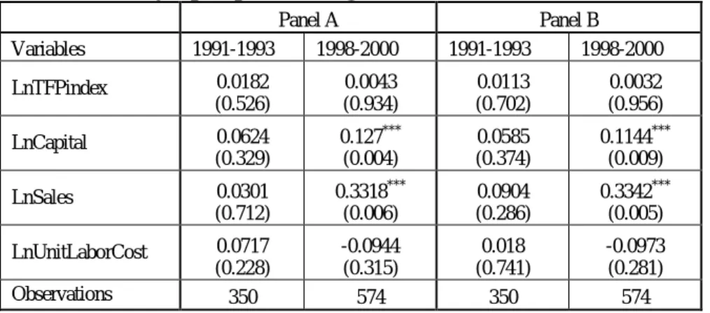
Export-starters display no empirical evidence that they count on pre export-market entry superior characteristics. Table 6 shows that the economic magnitudes of
total factor productivity, sales, capital, and (surprisingly) unit labor cost growth rate premiums are statistically insignificant at all conventional levels although they have positive coefficients between 1991 and 1993. During 1998 and 2000, the difference between exporters and non-exporters sales growth is 33%, and capital accumulation differential was 11%. Also, the coefficient of the unit labor cost has a negative (expected) but statistically insignificant sign. Moreover, the differential between exporters and non-exporters productivity growth is not statistically significant although the stock of capital increased. These observations allow concluding that non-exporters are inferior to export starters before the latter enter export markets. During 1998-2000, the stock of capital grows faster for export starters, probably because of sales growth. Nevertheless, during pre-entry years, export starters do not display significant firm productivity improvements compared to non-exporters.
Table 6 displays the results. During 1991-1993, the growth rate premia for TFP, sales and capital are all positive, but statistically insignificant. Surprisingly, the coefficient of unit labor cost also has a positive sign; however, it is not significant. Thus, during the initial pre-entry period, there is no evidence that exporter-starters build upon their already-superior characteristics. During 1988-2000, exporters accumulate around 11-12 % more capital than non-exporters. This is accompanied by a sales growth differential of 33 %. In spite of this increase in capital stock, exporters’ productivity growth is not statistically different than non-exporters’ productivity growth. The unit labor cost has the expected sign in this period although it is insignificant. To sum up, the export-starters already have the competitive advantage over non-exporters before they enter export markets. However, they do not experience any major productivity
improvements compared to non-exporters during the pre-entry periods. Only during 1998-2000, the capital stock appears to grow more for export-starters, possibly due to positive sales growth during this period.
[Insert Table 6]
Export starters experience higher capital, sales, and TFP growth rates than non-exporters, suggesting that export activity enhances firm performance. Controlling for firm size, the capital accumulation growth rate of export-starters is 9-16% higher than exporters. And, between 1994 and 1996, the growth rate of TFP is 0.7% higher than non-exporters. Over the following 3 years this differential stays positive but with no statistical significance. However, between 2001 and 2004, the TFP differential (+1.38%) becomes statistically significant. Controlling for capital, growth rate of sales is 8-15% higher for exporters. Moreover, the coefficient of unit labor cost, during all years, holds the expected sign but remains statistically significant only during the first year (two years) after entry during 1991-1997 (1998-2004). For these periods, the export-starters’ ULC growth rate is 3.83 % (6.65 %) lower than non-exporters’ ULC growth.
A theoretically-reliable method to identify the effect of exporting and the pros of exporting on export-starters would require data on the performance of export-starters if they do not engage in export market. Given this data is not observable, the above indication carries a problematic implicit assumption. Recent literature addressed this obstacle within the heterogeneous firm model. The heterogeneous ingredients of firm productivity between exporters and non-exporters - i.e. Melitz (2003), Head and Reis (2003), as well as Helpman, Melitz and Yeaple (2004) - can act as an objection to the assumption of Bernard and Jensen (1999) that compares export-starters with all
non-exporters, considering all non-exporting firms can provide a counter-factual. The propensity score matching method, which provide a more precise control for comparison groups (i.e. exporters and non-exporters) differentials, tackles this heterogeneity issue. The next subsection summarizes the theoretical implications of matching techniques, and it shows the empirical results of its application.
III.D.2 Propensity Score Matching and Learning Effects
Technically, if identifies the change in TFP (or another firm characteristic) and
represents an indicator of whether firm exported for the first time
at time , then is the change in TFP at time ( ) following entry. A
systematic measurement of effects of entry into export markets requires a counterfactual.
Thus, the export entry causal effect on firm at time can be written as
where denotes the outcome for export-starters had they never entered export
markets. The main problem is that this outcome is not observable. Following Heckman et al. (1997), we define the average effect of exporting on export-starters as:
The appropriate identification of a counterfactual for the latter term in the above equation is a key determinant of the measurement quality. Assuming that a vector of observable firm characteristics can capture all the differences between export-starters and firms in this control group, we estimate this counterfactual by the corresponding average value of a control group of firms. Non-exporters, which perform comparably to export-starters before export-market entry, are a common choice in the related literature for this
y
0,1 it Expdummy i t y1i,ts ts s0 i ts y1i,ts 0 ,t s i y 0 ,t s i y
yi1,ts yi0,ts Expdummyit 1
E y1i,ts Expdummyit 1
E yi0,ts Expdummyit 1
control group. Thus, the appropriate counterfactual is . The goal of this matching technique is to identify a non-exporting firms group for which the variables distribution affecting the export decision is comparable to the export-starters relevant distribution. We adopt the propensity score (estimated probability of a firm to export given its characteristics) matching technique of Rosenbaum and Rubin (1983) given matching non-exporters with export-starters on n-dimensional vector of characteristics is unfeasible. The propensity score matching technique facilitates comparison between firms and makes matching feasible by summarizing pre-treatment characteristics of each subject into a single index variable, namely, propensity score.
As an initial step, we find the propensity score for all export-starters and non-exporters for 1991-1997 and 1998-2004 using a probit specification for each period as follows. We have used several different combinations of controls and earlier periods (t-2 and t-3) in the F(.) function. The resulting specification in equation (6) is the outcome of the algorithm described below.
(8)
where is the normal cumulative distribution function. The control variables include
sales, capital, ULC, company age, company age squared, and industry dummies. Let
denote the probability of exporting at time for firm , which is an export-starter. A
non-exporting firm , which is closest in terms of its propensity score to firm , is
selected as a match. More formally, this nearest-neighbor matching method requires that
at each point in time, a non-exporting firm is chosen based on the following criteria:
yi0,ts Expdummyit 0
E ) , ( ) 1 (Expdummyi,t FTFPi,t1 Controli,t1 P (.) F t i P, t i j i j
min
( , , ) 0 , , , t j t i Expdummy j t j t i p p p p t j The results from the radius matching method are almost identical. With radius matching, each treated unit is matched only with the control units whose propensity scores fall in a predefined neighborhood (the radius determines the length of the neighborhood) of the treated unit’s propensity score. Therefore, unlike the nearest neighborhood matching, the radius matching can potentially result in unmatched treated units. In the present case, several choices of reasonably small radii did not leave any unmatched treated units.
We follow Becker and Ichino (2002)’s algorithm to confirm that the probit specification is valid and that the optimal number of groups of firms in which the propensity scores and the means of company characteristics do not differ for the treated
(export-starter) and the control (non-exporter) units8. Initially, the nearest neighbor
matching method eliminates substantially different non-exporting firms, and matches 98 (91) non-exporting firms to 110 (93) export-starters during 1991-1997 (1998-2004). The second step is to divide these updated samples into equally spaced intervals such that within each interval, the average propensity scores of the treatment and control group do
not differ statistically. 1 Before the second step, after identifying the appropriate matches,
we estimated the probit specification again with only the matched sample to update the propensity scores of the remaining control and treated units. This resulted in similar scores for both groups. The first group during 1991-1997 (1998-2004) includes 54 (47) export-starters and 50 (45) non-exporters. The second group during 1991-1997 (1998-2004) includes 56 (46) export-starters and 48 (46) non-exporters.
In both periods, splitting the sample into two intervals satisfies this condition.
Subsequently, we run a simple t-test of difference of means for the pre-entry period t1
to see if the mean characteristics of firms in all these four groups do not differ statistically between the treated and control units, i.e., we test the samples for balancing hypothesis. The results in table 7 indicate that this constraint is satisfied and the identified two groups for each period consist of appropriately matched firms. All the P-values are greater than 0.1, thus, the hypothesis that the means of these variables are equal for export-starters and non-exporters is not rejected at any confidence level.
[Insert Table 7]
Having assured that the subgroups of firms include very similar control and treatment units, the final step is to estimate the differences in changes of firm characteristics in these four groups during the post-treatment period, i.e. export market entry. That is, we estimate regression equation (6) for these matched samples. Table 8 presents the results for these four different groups. Matching leads to substantially different post-entry results especially in terms of TFP growth premia from those in section III.D.1 with non-matched samples.
During the first 3 years of post export market entry, sales for export-starters increased, on average 11.4% faster, compared to their domestic rivals, across the four groups. Also, the growth premium of capital follows the same trend as for sales but with less statistically significant coefficient. For instance, the capital accumulation in both groups, between 1991 and 1997, shows that export-starters experience faster capital accumulation in the second year after export market entry - and the growth is continuous (3-4%) in the long run. Moreover, between 1998 and 2004, the capital accumulation grew faster - 7% - for export-starters during the first year after export market entry.
The coefficients of unit labor cost (ULC) premium are mainly statistically insignificant although they have the expected negative sign except for the 3-year growth premium in group 1. Table 8 shows that export-starters experience a statistically significant reduction (1.54 % and 1.17 %) in their ULC relative to non-exporters only during the period 1998-2004, and specifically during the first post market entry year. In addition, during 1998-2004, export-starters experience TFP gains (1.03 % and 1.34 %) only during the first post market entry year while the coefficient of TFP growth premium is positive but statistically insignificant for both groups during 1991-1997.
In a nutshell, the above empirical evidence fails to make the case that access to foreign markets via the exports channel enhances learning and productivity for Indian manufacturing firms. TFP of Export-starters did not enhance significantly, compared to TFP of non-exporters, in the long run. However, sales and capital accumulation scaled up when firms were able to engage in foreign markets along with their engagements in their domestic markets.
[Insert Table 8]
IV. Conclusion:
Economists have argued that “openness to trade” increases productivity and stimulates growth. They viewed participation in export markets as a prerequisite for economic growth in developing countries. However, neither the theoretical studies nor the empirical cross-country analyses have reached a consensus on the channels through which exports enhances economic growth This paper examines the question of whether firms self-select into the export market using an Indian firm-level panel dataset of balance sheets and
income statements spanning 14 years (1991-2004) and covering 33,510 domestically-owned manufacturing companies categorized by sectors. The analysis takes place in three primary steps. First, we estimate exporter premia, which measure the extent to which exporters outperform non-exporters in terms of TFP, capital, sales and unit labor cost. We find that Indian exporters are larger (in terms of sales), employ more capital, have lower unit labor costs and higher productivities than non-exporters. Second, we examine whether firms that become exporters already have their desirable characteristics prior to entering the export market. We find that firms that will ultimately become exporters perform better than non-exporters. Third, we examine (i) whether firms prepare for exporting by consciously choosing to undertake productivity-increasing activities and (ii) whether firm productivity enhances following export market participation. We do not find evidence for this preparation or improvement hypotheses.
The self-selection hypothesis implies that more productive firms become exporters as they can cover high fixed costs of entering and serving foreign markets, including costs related to networking and adapting to new quality standards. The other hypothesis is the learning-by-exporting. The paper applies matching techniques to target the Learning-by-exporting hypothesis. The aim is to improve the identification quality of post-entry comparative analysis of exporters and non-exporters. In few words, matching decreases selection-bias as it helps identify certain non-exporters group with similar pre market entry productivity as exporters.
The paper provides evidence that more successful firms are more likely to enter export markets, giving support to the self-selection hypothesis. The results are robust, mainly that firms that engage in foreign competition perform better than their domestic
competitors years before they enter export markets. However, there is weak evidence as to whether these exporting firms prepare themselves consciously for the international markets. On the learning-by-exporting front, the paper fails to show that exporters improve their productivity performance after they enter export markets. While the paper finds export benefits (mainly in sales and capital accumulation), it fails to establish positive evidence for the learning-by-exporting hypothesis.
On economic and trade policy levels, this paper shows that export policies targeting the less productive domestic firms in an economy - i.e. via export subsidy - may not lead to trade openness, especially if the only channel of trade openness lies within firm productivity growth.
Needless to mention, as discussed in the paper, that export market entry may increase sales, reduce unemployment, reduce probability of firm exist, and enhance firms learning opportunities (i.e. depending on export destinations). These further issues - along with the reasoning for why the magnitudes of the Indian estimated exporter premium are different than elsewhere in the literature - are left as topics for future research. Moreover, further research can examine the conditions under which learning from exporting may occur. For instance, it is commonly argued that firms will learn more from exporting to industrialized countries than they can from poorer countries, and they will learn more from exporting to dynamic and fast changing environments than from exporting to weak and static environments. In other words, whether most of the Indian exporters export to countries or environments that contained relatively few opportunities for learning is a question for further research.
References
Alvarez, Roberto and Ricardo A. Lopez (2005), Exporting and performance: Evidence from Chilean plants,
Canadian Journal of Economics, 38: 1384-1400.
Amin, Mohammad and Haidar, Jamal Ibrahim (2011), Trade Facilitation and Country Size. World Bank mimeo
Becker, Sascha O. and Andrea Ichino (2002), Estimation of average treatment effects based on propensity scores, Stata Journal, 2: 358-377.
Bernard, Andrew B. and J. Bradford Jensen (1995), Exporters, jobs, and wages in U.S. manufacturing: 1976-1987, Brookings Papers on Economic Activity: Microeconomics, 67-119.
Bernard, Andrew B. and J. Bradford Jensen (1999), Exceptional exporter performance: cause, effect, or both? Journal of International Economics, 47: 1-25.
Bernard, Andrew B. and Joachim Wagner (1997), Exports and success in German manufacturing, Review
of World Economics, 133: 134–157.
Bernard, Andrew B. and Joachim Wagner (2001), Export entry and exit by German firms, Review of World
Economics, 137: 105-123
Blalock, Garrick and Paul J. Gertler (2004), Learning from exporting revisited in a less developed setting,
Journal of Development Economics, 75: 397-416.
Clerides, Sofronis K., Saul Lach, and James R. Tybout (1998), Is learning by exporting important? Micro-dynamic evidence from Colombia, Mexico, and Morocco, Quarterly Journal of Economics, CXIII: 903-947.
Haidar, Jamal Ibrahim (2012). The Impact of Business Regulatory Reforms on Economic Growth. Journal
of the Japanese and International Economies, (forthcoming)
Haidar, Jamal Ibrahim (2009). Investors Protections and Economic Growth. Economics Letters, 103(1): 1-4.
Head, Keith and John Ries (2003), Heterogeneity and the FDWE versus export decision of Japanese manufacturers, Journal of the Japanese and International Economies, 17: 448-467.
Heckman, James J & Ichimura, Hidehiko & Todd, Petra E. (1997). Matching as an Econometric Evaluation Estimator: Evidence from Evaluating a Job Training Programme, Review of Economic Studies, 64(4): 605-54.
Helpman, Elhanan, Marc J. Melitz, and Stephen R. Yeaple (2004), Export versus FDWE with heterogeneous firms, American Economic Review, 94: 300-316.
Kraay, Aart (2002), Exports and economic performance: evidence from a panel of Chinese enterprises, in Mary-Francoise Renard, eds., China and its Regions. Economic Growth and Reform in Chinese
Provinces: 2002. Cheltenham, Elgar.
Levinsohn, James and Amil Petrin (2003), Estimating production functions using inputs to control for unobservables, Review of Economic Studies, 70: 317-342.
Melitz, Marc J. (2003), The impact of trade on Iintra-industry reallocations and aggregate industry productivity, Econometrica, 71: 695-1725.
Roberts, Mark J. and James R. Tybout (1997), The decision to export in Colombia: An empirical model of entry with sunk costs, American Economic Review, 87: 545-564.
Robinson, Peter M. (1988), Semi-parametric econometrics: A survey, Journal of Applied Econometrics, 3: 35-51.
Rosenbaum, P. R., and Rubin, D. B., (1983), The Central Role of the Propensity Score in Observational Studies for Causal Effects. Biometrika 70, 41–55.
Serti, Francesco and Chiara Tomas (2008), Self-selection and post-entry effects of exports: Evidence from Italian manufacturing firms, Review of World Economics, 144: 660-694.
Topalova, Petia (2004), Trade liberalization and firm productivity: The case of India, IMF Working Papers 04: 28.
Wagner, Joachim (2007), Exports and productivity: A survey of the evidence from firm-level data, The
Table 1: Export patterns of manufacturing firms
Year Number of firms Exporters (%) Entrants (%)
Quitters (%) 1991 2010 55.8 5.3 2.6 1992 2112 57.4 7.8 2.6 1993 2166 55.7 5.8 2.5 1994 2796 54 6.8 2.3 1995 3367 53.6 7.8 2.5 1996 3538 55.1 7.2 3.6 1997 3512 55.4 5.8 5.2 1998 3522 56 4.6 4.1 1999 3797 53.8 4.2 4.4 2000 4007 52.3 4.5 5.2 2001 3944 52.8 5.6 4.7 2002 4000 52.3 4.5 4.4 2003 4136 53.2 4.4 3.7 2004 3980 56.3 5.1 3.5
Table 2: Descriptive statistics for exporters and non-exporters
Observations Mean St. Dev. Minimum Maximum Variables (exporters)
Sales 16,857 315.97 2,685.43 0.00 159,984.40
Total income 16,857 323.46 2,736.81 -7.40 162,755.20 Raw material expenses 16,857 116.80 971.51 -6.77 55,826.18 Power and fuel expenses 16,857 13.78 72.22 0.00 3,389.74 salaries and wages 16,857 19.87 113.45 0.00 5,176.53
Capital 16,857 218.61 1,686.69 0.00 90,204.68 company age 16,134 28.82 75.14 0.00 181.00 TFP index 16,207 0.24 0.69 -5.27 8.84 Variables (non-exporters) Sales 16,653 54.61 349.64 0.00 26,966.30 Total income 16,653 56.28 359.79 -18.76 27,388.14 Raw material expenses 16,653 23.81 198.32 -5.95 19,645.06 Power and fuel expenses 16,653 3.80 23.49 0.00 1,551.34 Salaries and wages 16,653 4.61 38.58 0.06 1,625.04
Capital 16,653 59.31 558.95 0.00 46,231.60
Company age 16,653 24.90 94.87 0.00 172.00
Table 3: Export Premium OLS regression of log values of firm characteristics on export status 1991 1992 1993 1994 1995 1996 1997 1998 1999 2000 2001 2002 2003 2004 LnTFP 0.186*** (0.000) 0.165*** (0.000) 0.168*** (0.000) 0.155*** (0.000) 0.157*** (0.000) 0.111*** (0.000) 0.095*** (0.000) 0.059** (0.031) 0.078*** (0.003) 0.129*** (0.000) 0.115*** (0.000) 0.090*** (0.003) 0.088*** (0.003) 0.090*** (0.003) LnCapital 1.253*** (0.000) 1.118*** (0.000) 1.542*** (0.000) 1.861*** (0.000) 1.925*** (0.000) 1.987*** (0.000) 2.179*** (0.000) 2.455*** (0.000) 2.525*** (0.000) 2.557*** (0.000) 2.807*** (0.000) 3.221*** (0.000) 3.085*** (0.000) 3.396*** (0.000) LnSales 1.734*** (0.000) 1.735*** (0.000) 2.066*** (0.000) 2.422*** (0.000) 3.056*** (0.000) 2.827*** (0.000) 3.219*** (0.000) 3.38*** (0.000) 4.163*** (0.000) 4.632*** (0.000) 5.18*** (0.000) 6.120*** (0.000) 5.80*** (0.000) 6.215*** (0.000) LnUnitLaborCost - 0.068 (0.127) - 0.055 (0.214) - 0.094** (0.027) - 0.190*** (0.000) - 0.187*** (0.000) - 0.159*** (0.000) - 0.128*** (0.000) 3.38*** (0.000) 4.163*** (0.000) 4.632*** (0.000) 5.180*** (0.000) 6.120*** (0.000) 5.80*** (0.000) 6.215*** (0.000) Observations 1986 2050 2110 2724 3285 3478 3459 3465 3728 3946 3902 3949 4058 3864
Note: P-values are reported in parenthesis below the estimates. ** and *** refer to 5% and 1% statistical significance levels, respectively. The reported export premium estimates are the exact percentage differentials given by (e^β-1)*100 where β is the export dummy coefficient from regression equation (2). All regressions include industry dummies and company age (in log). The TFP and unit labor cost regressions include a firm size dummy.
Table 4: Export Premium OLS regression of log values of firm characteristics on export status and firm-specific controls (in logs) 1991 1992 1993 1994 1995 1996 1997 1998 1999 2000 2001 2002 2003 2004 LNTFP 0.224*** (0.000) 0.196*** (0.000) 0.213*** (0.000) 0.227*** (0.000) 0.225*** (0.000) 0.240*** (0.000) 0.235*** (0.000) 0.196*** (0.000) 0.217*** (0.000) 0.272*** (0.000) 0.267*** (0.000) 0.251*** (0.000) 0.256*** (0.000) 0.261*** (0.000) LnCapital 0.731*** (0.000) 0.526*** (0.000) 0.763*** (0.000) 0.972*** (0.000) 0.887*** (0.000) 0.867*** (0.000) 0.955*** (0.000) 1.055*** (0.000) 1.036*** (0.000) 0.974*** (0.000) 1.071*** (0.000) 1.182*** (0.000) 1.135*** (0.000) 1.363*** (0.000) LnSales 0.54*** (0.000) 0.519*** (0.000) 0.567*** (0.000) 0.634*** (0.000) 0.865*** (0.000) 0.645*** (0.000) 0.693*** (0.000) 0.670*** (0.000) 0.953*** (0.000) 1.169*** (0.000) 1.222*** (0.000) 1.284*** (0.000) 1.392*** (0.000) 1.392*** (0.000) LnUnitLaborCost - 0.070 (0.123) - 0.056 (0.209) - 0.092** (0.030) - 0.193*** (0.000) - 0.184*** (0.000) - 0.148*** (0.000) - 0.121*** (0.001) 0.670*** (0.000) 0.953*** (0.000) 1.169*** (0.000) 1.222*** (0.000) 1.284*** (0.000) 1.392*** (0.000) 1.392*** (0.000) Observations 1986 2050 2110 2724 3285 3478 3459 3465 3728 3946 3902 3949 4058 3864
Note: P-values are reported in parenthesis below the estimates. ** and *** refer to 5% and 1% statistical significance levels, respectively. The reported export premium estimates are the exact percentage differentials given by (e^β-1)*100 where β is the export dummy coefficient from regression equation (2). All regressions include industry dummies and company age (in log). The TFP controls for capital stock in addition to firm size. The capital regressions control for firm size and the sales regressions control for capital stocks. (Firm size dummy is left out since it is constructed based on sales). The unit labor cost regressions include both a firm size and capital.
Table 5: Characteristics of export starters Variables 1991 1992 1993 1998 1999 2000 LnTFPindex 0.278** (0.012) 0.289** (0.017) 0.322*** (0.007) 0.34** (0.013) 0.335** (0.021) 0.326*** (0.039) LnCapital 1.476*** (0.004) 1.686*** (0.001) 1.809*** (0.000) 1.595*** (0.003) 2.41*** (0.000) 2.76*** (0.000) LnSales 3.232*** (0.000) 2.552*** (0.000) 2.493*** (0.000) 2.91*** (0.000) 4.027*** (0.000) 5.565*** (0.000) LnUnitLaborCost - 0.488*** (0.000) - 0.373*** (0.002) - 0.382*** (0.001) - 0.409** (0.039) - 0.346* (0.072) - 0.508*** (0.005) Observations 350 350 352 576 580 582
Note: P-values are reported in parenthesis below the estimates. *, **, and *** refer to 10%, 5% and 1% statistical significance levels, respectively. The reported export premium estimates are the exact percentage differentials given by (e^β-1)*100 where β is the export dummy coefficient from regression equation (6). All regressions include industry dummies and company age (in log). The TFP and unit labor cost regressions include a firm size dummy. Industry and year interacted fixed effects controls are included.
Table 6: Pre-entry export premium of growth rates Panel A Panel B Variables 1991-1993 1998-2000 1991-1993 1998-2000 LnTFPindex 0.0182 (0.526) 0.0043 (0.934) 0.0113 (0.702) 0.0032 (0.956) LnCapital 0.0624 (0.329) 0.127*** (0.004) 0.0585 (0.374) 0.1144*** (0.009) LnSales 0.0301 (0.712) 0.3318*** (0.006) 0.0904 (0.286) 0.3342*** (0.005) LnUnitLaborCost 0.0717 (0.228) -0.0944 (0.315) 0.018 (0.741) -0.0973 (0.281) Observations 350 574 350 574
P-values are reported in parenthesis below the estimates. *** refer to 1% statistical significance level. The reported export premium estimates are the exact percentage differentials given by (e^β-1)*100 where β is the export dummy coefficient from regression equation (8). All regressions include industry dummies and company age (in log). The TFP and unit labor cost regressions include a firm size dummy in panel A. The TFP controls for capital stock in addition to firm size in panel B. The capital regressions control for firm size and the sales regressions control for capital stocks (firm size dummy is left out since it is constructed based on sales) and the unit labor cost regressions include both a firm size and capital. Industry and year interacted fixed effects controls are included.
Figure 7: Basic data characteristics of non-exporters and exporters in the matched samples Matched sample (1991-1997) Matched sample (1998-2004)
Group 1 Group 2 Group 1 Group 2
Variable Difference in Means Difference in Means
TFP 0.013 0.025 0.106 0.041 (0.540) (0.423) (0.554) (0.643) Capital 0.022 0.138 0.056 0.232 (0.785) (0.251) (0.182) (0.611) Sales 0.125 0.117 0.129 0.223 (0.332) (0.721) (0.294) (0.336) ULC -0.241 -0.003 -0.247 -0.095 (0.152) (0.224) (0.183) (0.151)
The differences of means are calculated by subtracting the means of the relevant variables of non-exporters from the means of the corresponding variables of exporter-starters. Numbers in brackets refer to p-values. P-values refer to the t-tests performed for the equality of means, for which the null hypothesis is that the selected groups do not differ in population means.
Table 8: Post-entry export premium of growth rates - Matched samples
Group 1 (1991-1997) Growth Rate Group 2 (1991-1997) Growth Rate Group 3 (1998-2004) Growth Rate Group 4 (1998-2004) Growth Rate Variables 1994-1995 1994-1996 1994-1997 1994-1995 1994-1996 1994-1997 2001-2002 2001-2003 2001-2004 2001-2002 2001-2003 2001-2004 Log TFP index 0.0072 0.0084 0.0033 0.0060 0.0116 0.0012 0.0103** 0.0127 0.0085 0.0134* 0.0108 0.0095 (0.163) (0.122) (0.293) (0.238) (0.390) (0.259) (0.017) (0.246) (0.192) (0.068) (0.126) (0.230) Log Capital 0.0653 0.0727** 0.0415* 0.0702 0.0539** 0.0322*** 0.0787*** 0.0756** 0.0559 0.0688** 0.0731** 0.0604 (0.123) (0.030) (0.078) (0.159) (0.023) (0.004) (0.002) (0.015) (0.120) (0.015) (0.018) (0.240) Log Sales 0.0704* 0.0985** 0.1119*** 0.0745*** 0.0922** 0.1098** 0.0884*** 0.0855*** 0.1014** 0.0762*** 0.0808*** 0.0923** (0.055) (0.017) (0.007) (0.002) (0.011) (0.013) (0.002) (0.004) (0.024) (0.006) (0.001) (0.038) Log ULC -0.0133 -0.0108 0.0038 -0.0172 -0.0099 -0.0057 -0.0154** -0.0122 -0.0094 -0.0117** -0.0137 -0.0105 (0.230) (0.512) (0.281) (0.348) (0.454) (0.532) (0.033) (0.245) (0.385) (0.025) (0.158) (0.293) Observations 104 102 102 102 102 100 92 92 92 92 90 92
All regressions include dummies and company age (in log). The above figures include a firm size dummy for TFP regressions and ULC regressions. P-values are in parentheses. ** and *** refer to 5% and 1% statistical significance levels, respectively.