HAL Id: hal-00735123
https://hal-ifp.archives-ouvertes.fr/hal-00735123
Submitted on 25 Sep 2012HAL is a multi-disciplinary open access archive for the deposit and dissemination of sci-entific research documents, whether they are pub-lished or not. The documents may come from teaching and research institutions in France or abroad, or from public or private research centers.
L’archive ouverte pluridisciplinaire HAL, est destinée au dépôt et à la diffusion de documents scientifiques de niveau recherche, publiés ou non, émanant des établissements d’enseignement et de recherche français ou étrangers, des laboratoires publics ou privés.
Mathieu Feraille, Amandine Marrel
To cite this version:
Mathieu Feraille, Amandine Marrel. Prediction under Uncertainty on a Mature Field. Oil & Gas Science and Technology - Revue d’IFP Energies nouvelles, Institut Français du Pétrole, 2012, 67 (2), pp.193-206. �10.2516/ogst/2011172�. �hal-00735123�
Prediction under Uncertainty on a Mature Field
M. Feraille and A. Marrel*
IFP Energies nouvelles, 1-4 avenue de Bois-Préau, 92852 Rueil-Malmaison Cedex - France e-mail: [email protected] - [email protected]
* Now works at CEA Cadarache
Résumé – Prévision de production sous incertitude pour un champ mature – Dans le cadre de
l’ingénierie de réservoir, des simulateurs permettent de comprendre et prédire le déplacement des fluides dans le réservoir et ainsi d’optimiser son exploitation. Ces simulateurs prennent en entrée un grand nombre de paramètres qui peuvent être entachés d’incertitudes. Afin d’assurer une production future correcte, la comparaison des différents scénarios d’exploitation possibles doit tenir compte de ces incertitudes. Les prévisions de production ne doivent pas être évaluées en ne considérant qu’un seul cas « moyen » pour chaque scénario mais en intégrant l’incertitude sur les paramètres d’entrée. Dans le cadre de champ mature où un historique de production est disponible, le formalisme Bayésien est bien adapté pour répondre au problème des prédictions sous incertitudes. En effet, il permet de définir les incertitudes, dites a posteriori, sur les entrées du modèle de réservoir en prenant en compte à la fois les données statiques et dynamiques. Ces incertitudes a posteriori peuvent ensuite être propagées afin de calculer des prévisions de production probabilistes pour chaque scénario, tout en respectant la connaissance statique et dynamique du réservoir. Mais l’obtention des incertitudes a posteriori ainsi que la propagation de celles-ci sur les prévisions de production nécessitent un nombre souvent prohibitif de simulations du modèle réservoir.
Dans cet article, nous proposons une application de plusieurs techniques statistiques avancées afin de prendre en compte les incertitudes dans les prévisions de production pour un champ mature et ce en utilisant un nombre raisonnable de simulations. Le champ mature considéré est le modèle de réservoir PUNQS qui a été utilisé auparavant dans plusieurs études comparatives de quantification d’incertitudes et de calage d’historique. Une méthodologie basée sur trois étapes est proposée et appliquée au cas PUNQS. Tout d’abord, une sélection et une analyse de sensibilité ont été réalisées afin de déterminer les paramètres d’entrée incertains les plus influents. Puis, dans une seconde étape, une méthode d’inversion probabiliste a été utilisée afin de réduire l’incertitude sur les paramètres en estimant leur incertitude
a posteriori. Enfin, des prédictions probabilistes au-delà des données d’historique sont calculées en propageant les incertitudes a posteriori des paramètres. Au cours de la première étape, deux techniques d’analyse de sensibilité sont proposées et comparées. L’une, qualitative, basée sur la méthode Morris et une autre, plus quantitative, basée sur les indices de Sobol. Au cours de la deuxième étape, une procédure de calage probabiliste est utilisée afin de réduire l’incertitude. La méthode proposée repose sur une modélisation par surface de réponse non paramétrique de type processus gaussien et sur une stratégie de planification adaptative. Dans la dernière étape, des surfaces de réponse paramétriques sont utilisées afin de modéliser les prévisions de production de réservoir et obtenir leur répartition probabiliste en propageant l’incertitude a posteriori des paramètres d’entrée.
Abstract – Prediction under Uncertainty on a Mature Field – Reservoir engineering studies involve a large number of parameters with great uncertainties. To ensure correct future production, a comparison of possible scenarios in managing related uncertainties is needed. Comparisons can be performed with more information than only a single mean case for each scenario. The Bayesian formalism is well
Monitoring of CO2Sequestration and Hydrocarbon Production Monitoring pour le stockage du CO2et la production des hydrocarbures
INTRODUCTION
The selection of the best development plan among several possible scenarios is a classical reservoir engineering problem. This task involves the comparison of possible scenarios. Comparisons based only on a single mean case for each scenario can lead to wrong conclusions. Thus, including uncertainty assessment for each scenario is necessary to avoid misleading conclusions. For mature fields, the Bayesian formalism is well tailored to compute posterior uncertainty while taking into account static and dynamic data. This posterior uncertainty can then be propagated to compute probabilistic production forecasts for each possible future development scenario. To achieve these different objectives while avoiding a prohibitive number of reservoir simulations, several advanced statistical methods are proposed in this paper. Thus, we aim at providing a global methodology to manage the uncertainty on a mature reservoir [1].
Uncertainty in reservoir engineering studies is associated with many input parameters of the geological-to-fluid flow reservoir workflow. These input parameters are considered as variables in a statistic framework. The aim of the proposed methodology is to take into account production data to reduce the uncertainty on input parameters and to perform probabilistic production forecasts associated with the remaining input uncertainty. This is achieved by performing qualitative and quantitative studies, using different statistical techniques. The methodology that we propose is based on three steps:
– Step 1: Identify and select the most influential uncertain
parameters using the match between simulated and mea-sured production data. To evaluate the mismatch between production and simulated data, an Objective Function (OF) is defined. Then, two different techniques of Global
Sensitivity Analysis (GSA) are proposed and compared to perform the sensitivity analysis of the OF. The first one is based on the Morris method [2, 3] which is a screening method leading to qualitative results. The second one is based on the computation of Sobol’ indices [4] and pro-vides more quantitative results. In the case of computa-tionally expensive simulations, direct sampling methods (Monte Carlo) which require thousands simulations are impractical. To deal with these expensive models, a Non-Parametric Response Surface (NPRS) approach can be used. The Gaussian process model is a widely used NPRS to approximate responses of numerical models or to per-form optimization. Previous works such as [5-12] describe how a Gaussian process, possibly associated with adaptive design, can be used to perform uncertainty management on fluid flow models, such as to propagate input uncer-tainty on output results and to perform sensitivity analysis. In [13-17], a Gaussian process is used to approximate the Objective Function in a local, global or Bayesian opti-mization purpose. Thus, we propose to use the Gaussian process model associated with an adaptive design strategy [12] to estimate the Sobol’ indices and identify the most influential uncertain parameters. Then only the selected uncertain parameters are used for the next two steps;
– Step 2: Compute a representative set of all possible
matched models through the application of the Bayesian formalism [18] to determine the posterior uncertainty of influential parameters. As it requires generally many thousands of simulations of the fluid flow model to get this posterior distribution, a NPRS approach with an adap-tive design strategy is proposed [15-17]. The adapadap-tive design strategy used to select new simulations is based on Markov Chain Monte Carlo sampling combining, at each
tailored to address the key problem of making predictions under uncertainty, especially in mature fields. It enables to define the reservoir uncertainty taking into account static and dynamic data. This posterior uncertainty can then be propagated to compute probabilistic production forecasts for each scenario, while honoring static and dynamic knowledge of the reservoir. But obtaining posterior uncertainty, as well as propagating it on production forecasts, entails a prohibitive number of reservoir simulations. In this paper, we propose an application of several advanced statistical techniques to perform prediction under uncertainty on a mature field using a reasonable number of simulations. The considered mature field is the PUNQS reservoir model which has been previously used in several comparison studies on uncertainty quantification and history-matching. A workflow based on three steps has been applied. First, a screening and a sensitivity analysis were performed to find the most influential parameters. Then, a probabilistic inversion method was used to reduce uncertainty on the parameters by estimating their posterior uncertainty. Finally, probabilistic predictions are computed by propagating the reduced uncertainty of parameters. In the first step of the workflow, two different sensitivity techniques are discussed and compared. One, more qualitative, based on the Morris method and another, more quantitative, based on Sobol’ indices. In the second step, a probabilistic history-matching procedure is applied to reduce the uncertainty. It is based on both a non parametric response surface approach which uses Gaussian process modeling and an adaptive design strategy. In the final step of the workflow, parametric response surfaces are used to approximate the reservoir production forecasts and obtain their probabilistic distribution by propagating the remaining posterior uncertainty of input parameters.
iteration, a global search for the optimum based on the Expected Improvement method [13, 14] and an explo-rative search. Finally, this history-matching step results in a reduction of the input uncertainty;
– Step 3: Perform the probabilistic production forecasts for
four more years after the history-matching period, propa-gating the remaining input uncertainty. To avoid, again, a huge number of simulations, parametric response surfaces are used to approximate the reservoir production forecasts [19] and propagate via Monte Carlo sampling the remaining posterior uncertainty of input parameters [15-17]. Probabilistic distributions for production fore-casts are so provided.
All the methodology that we propose is more precisely detailed in what follows (one section for each step). This methodology is applied to a reservoir test case which is, at first, described in the next section.
1 TEST CASE AND UNCERTAIN PARAMETERS
The test case of this paper is derived from the PUNQS case which was originally used for comparative inversion studies in the European PUNQS project [1].
The top structure of the reservoir is shown in Figure 1. The reservoir is surrounded by an aquifer in the north and the
west, and delimited by a fault in the south and the east. A small gas cap is initially present. The geological model is composed of five independent layers, three of good quality (layers 1, 3 and 5) and two of poorer quality. There are six production wells. A multiphasis fluid flow simulator is used to forecast the reservoir production.
The following 20 independent parameters, characteristic of media, rocks, fluids or aquifer activity, are defined within the fluid flow model and considered as uncertain. Note that, the hypothesis of independency between the parameters is physically acceptable. Table 1 summarizes for each parameter its name, uncertainty ranges, unit and description, as well as its value, specified in the column “History Data Point”, to create fictitious history data.
The fictitious production data correspond to the simulated production results performed using the values of the parame-ters specified in the column “History Data Point” of Table 1. These production data correspond to water cut, oil rate and gas oil ratio of all the wells from 0 to 2 922 days (i.e. 8 years). Production data for more than eight years are simu-lated. The remaining time steps are used to further check the probabilistic prediction quality.
2 STEP 1: SELECTION OF THE MOST INFLUENTIAL PARAMETERS FOR HISTORY-MATCHING
Reservoir engineering studies involve a large number of parameters with large uncertainty ranges. Finding a good history-matching solution in such a large uncertain parameter domain could be overwhelming. Therefore, a Global Sensitivity Analysis (GSA) is necessary to identify a reduced number of influential parameters on history-matching. 2.1 Definition of the Objective Function
At the beginning of our study, 20 uncertain parameters were identified as having a possible impact on the match. To find the most influential ones, an Objective Function (OF) mea-suring the mismatch between production and simulated data was defined. The OF is built using classical weighted least square formula:
(1) where f is the simulator, ydatathe production data, k, j and t
are respectively the production wells, the properties (water cut, oil rate and gas oil ratio) and the time index (each year during the eight first years of production). For each data series (one well and one property), a confidence interval is estimated at 10% of its mean. The weights are given by the inverse of the square of these confidence intervals divided by the number of time steps in each data series.
Two different GSA techniques are proposed and discussed: one, more qualitative based on the Morris method,
OF x wkj f x y j k kjt data kjt t ( )=1
∑
∑
∑
( ( )− ) 2 2 2339 Tops 2347 2355 2369 2371 2379 2387 2395 2403 2411 2 000 4 000 PUNQS FAULT XY plane 1 0 800 X3 X1 X5 X4 X2 GOC PRO-1 PRO-4 PRO-11 PRO-15 PRO-5 PRO-12 OWC 1 600 2 400 3 200 Figure 1and another, more quantitative based on the variance decom-position (estimation of Sobol’ indices) using a NPRS approach and an adaptive design.
2.2 Screening by the Morris Method
The screening method, introduced in [2], is used to identify the influential parameters on a response (in our case the OF) of a model.
Let us consider Y = f (X) the response of a model f (i.e. computer code). The input variables or parameters are ran-dom and modeled by the ranran-dom vector X = (X1, ..., Xd)∈ ℜd,
of known distribution. We note x = (x1, ..., xd) and y realizations
of X and Y.
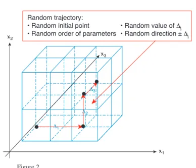
A Morris design is structured in sets of points, called trajectories. These trajectories are random, but follow a specific scheme:
– the trajectories are one-factor-at-a-time, thus two succes-sive points differ by one parameter only;
– for each trajectory, each parameter varies exactly once between two successive points.
To build a Morris design, the parameters are considered as discrete with different number of possible levels. A grid
of possible points is therefore defined. Figure 2 shows a trajectory generated for a case with three uncertain parame-ters X1(4 levels), X2(3 levels), and X3(3 levels). An initial point is randomly chosen on the grid and each coordinate
x1 x3 x2 Δ3 Δ2 Δ1 Random trajectory: • Random initial point • Random order of parameters
• Random value of Δj • Random direction ± Δj
Figure 2
Example of one trajectory built using the Morris method. TABLE 1
Uncertain parameters
Name History data point Min. Max. Unit Description
DensityGas 0.889 0.8 0.9 kg/m3 Gas density
DensityOil 932.323 900.0 950.0 kg/m3 Oil density
MPH1 1.03 0.8 1.2 Horizontal permeability multiplier for layer 1
MPH2 0.816 0.8 1.2 Horizontal permeability multiplier for layer 2
MPH3 0.861 0.8 1.2 Horizontal permeability multiplier for layer 3
MPH4 0.897 0.8 1.2 Horizontal permeability multiplier for layer 4
MPH5 1.115 0.8 1.2 Horizontal permeability multiplier for layer 5
MPV1 0.885 0.8 1.2 Vertical permeability multiplier for layer 1
MPV2 1.172 0.8 1.2 Vertical permeability multiplier for layer 2
MPV3 0.816 0.8 1.2 Vertical permeability multiplier for layer 3
MPV4 0.865 0.8 1.2 Vertical permeability multiplier for layer 4
MPV5 1.038 0.8 1.2 Vertical permeability multiplier for layer 5
PermAqui1 172.727 100.0 200.0 mD Permeability of aquifer 1
PermAqui2 177.778 100.0 200.0 mD Permeability of aquifer 2
PoroAqui1 0.282 0.2 0.3 % Porosity of aquifer 1
PoroAqui2 0.276 0.2 0.3 % Porosity of aquifer 2
SGCR 0.073 0.02 0.08 Critical gas saturation
SOGCR 0.164 0.15 0.2 Critical oil-gas saturation
SOWCR 0.187 0.15 0.2 Critical oil-water saturation
xiis successively increased or decreased at a random value Δi, where Δiis a multiple of the grid spacing in direction i.
In the case of d uncertain parameters, each trajectory is composed by (d + 1) points. L random trajectories are built following the same scheme and the random design thus gen-erated has L× (d + 1) sampling points. After having launched the simulations associated to the points of the Morris design, it is possible to compute, for each trajectory, an elementary effect of each input parameter:
This elementary effect corresponds to the variation of the response when the considered parameter is moved while the others are fixed. It can be viewed as some discrete derivative. For each input, two sensitivity measures are computed by post-processing the elementary effects: its absolute mean and standard deviation:
– the absolute mean µi*of {d
i(l)}l = 1, ..., Lassesses the overall
influence of the input parameter Xion the response Y:
(3) The interpretation of µi*is quite simple: if µi*is low, the
average elementary effect of the input xi is negligible so xi
has no effect on y and if µi*is high, the input Xihas a
sig-nificant effect on Y. Note that the mean of the elementary effect can also be used and can give additional information such as the sense of variation of parameter influences;
µi il l L L d d ∗ = =1
∑
=1 1 ( ) , for i ..., d y x x x x i l l i l i l i l ( ) ( ) ( ) ( ) ( ) ( , ..., , , = + − 1 1 Δ ii l d l l i l x y x x +1 − 1 ( ) ( ) ( ) ( ) , ..., ) ( , ..., , . ..., ( )) ( ) for , ..., and x i d d l i l Δ = 1 ll= 1, ..., L– the standard deviation σiof {di(l)}l = 1, ..., Lestimates the
non-linear and/or interaction effects of the parameter Xion
the response Y:
(4) Consequently, if σi is low, the input Xi does not have
neither non-linear nor interaction effect on the response Y. So, if µi*is high and σiis low, Xihas only a linear effect
on Y. On the contrary, if σiis high, the input Xihas a
non-linear effect and/or interaction effect on the response Y. The Morris method is now applied on the OF in order to determine, among the 20 uncertain parameters, the influential ones on the mismatch of the mature field. A Morris design is built with five trajectories and five levels for each parameter, leading to a total number of 5× (1 + 20) = 105 simulations. The OF values associated with the 105 simulations are shown in Figure 3. The variation range observed for these
OFvalues is [50; 2 000].
To determine the most influential parameters on this OF, the Morris post treatment is performed: σiand µi*are computed
and plotted on the same graph. This Morris plot representing
(µi*, σi)i = 1, …, dis shown in Figure 4.
By graphically analyzing the high and low values of σi
and µi*, the parameters are split into two groups: the
influen-tial and the negligible parameters on the OF. We can show that 10 parameters (MPH5, MPH1, PermAqui1, SWCR, MPH4, PoroAqui1, MPV4, MPH3, SGCR and SOWCR) among 20 are potentially influential on the OF through linear effects and interaction or non-linear effects. Thus, the pres-ence of non-linear effects or interactions justifies the compu-tation of Sobol’ indices to perform quantitative sensitivity
σi il µ i l L L d d = −
∑
=(
−)
= 1 1 1 2 1 ( ) , for i ...,E1 E5 E9 E14 E19 E24 E29 E34 E39 E44 E49 E54 E59 E64 E69 E74 E79 E84 E89 E94 E99 E105
OF 1 1 100 300 500 700 1 500 1 700 1 900 900 1 100 1 300 Simulations OF 1 (objective function) Figure 3
OFvalues associated to the 105 simulations of the Morris design.
analysis, compared to easiest quantitative sensitivity methods based on linear regression or rank-based linear regression [20].
2.3 Variance-Based GSA with a Non-Parametric Response Surface
2.3.1 Definition of Sobol’ Indices
Compared to screening techniques such as Morris, GSA based on variance decomposition enables to perform quanti-tative sensitivity analysis.
Indeed, variance-based GSA provides measures that deter-mine the precise part of response variability explained by each variable Xi and any interaction between variables [4].
These measures, known as the Sobol’ indices, are based upon the functional analysis of variance (ANOVA) decomposition of any square integrable function [21]. Sobol’ indices can handle nonlinear and non-monotonic relationships between inputs and output and are defined as:
(5)
Siwhich is the first order Sobol index measures the part of
the response variance explained by Xialone. Siis also called
the primary effect of Xi. Similarly, Sijdefined for i ≠ j
mea-sures the part of response variance due to the interaction
Sij Var E Y X X i j =
(
)
⎡ ⎣ , ⎤⎤⎦( )
− − = Var Y Si Sj, Sijk ... S Var E Y X Var Y i i = ⎡⎣(
)
⎤⎦( )
,effect between Xiand Xj. In an equivalent way, higher order
indices can be defined.
The interpretation of Sobol’ indices is natural. They are all included in the interval [0; 1] interval and their sum is one in the case of independent input variables. The closer to 1 the Sobol’ index is, the greater is the part of response variance due to the input variable related to this index.
To express the overall response sensitivity to an input Xi
the total sensitivity index STi, also called total effect is
intro-duced in [22]. STiis defined as the sum of all the sensitivity
indices involving Xi:
(6) where k # i denotes all the terms that include the index i.
Computational techniques (FAST, quasi-Monte Carlo, etc. [23]) exist to estimate efficiently the first and total sensitivity indices. In particular, STican be estimated without computing
each sensitivity indices for all orders. In practice, only Siand STiare generally estimated.
2.3.2 Description of the Non-Parametric Response Surface Construction and Adaptive Sampling Strategy
When Y is related to outputs of a fluid flow simulator (or any black box simulator), such as our OF, the estimation of the sensitivity indices requires too many evaluations of Y and cannot be applied directly. Thus, Y can be approximated by a predictive Response Surface (RS) built using a limited num-ber of simulations. This RS approximation of Y which requires a negligible computer time for evaluation is then
STi Sk k i =
∑
# 0.1 0 0.2 0.3 0.4 0.5 Density gas Density oil MPH1 MPH2 MPH3 MPH4 MPH5 MPV1 MPV2 MPV3 MPV4 MPV5 PermAqui1 PermAqui2 PoroAqui1 PoroAqui2 SGCR SOGCR SOWCR 0.7 0.6 0.5 0.4 0.3 0.2 0.1 0OF 1 (objective function) OF 1 (objective function)
σ σ 0 0.1 0.2 0.3 0.4 0.5 0.6 0.7 0.8 0.9 1.1 1.0 0.9 0.8 0.7 0.6 0.5 0.4 0.3 0.2 0.1 0 μ* μ* Influential parameters Negligible parameters Figure 4
used to replace the fluid flow simulator when computing the sensitivity indices. Among all the RS-based solutions for numerical simulators (linear regression, polynomials, splines, neural networks, etc.), the Gaussian process approach is one of the most popular due to the wide range of applications where it was successfully used [7, 24, 25]. Moreover, the presence of potential non-linear effects and interactions between the OF and the uncertain input parameters requires the use of more advanced and efficient RS than a simple lin-ear regression. Previous works such as [5-11] describe how Gaussian Process (GP), possibly associated with adaptive design, can be used to approximate outputs of a fluid flow model. In this paper, we use a RS based on GP technique combined with an adaptive design as detailed in [12] and roughly described below.
In what follows, we denote Non-Parametric Response Surface (NPRS), the RS build using GP. The number of nec-essary points to build a predictive NPRS depends on the complexity of the function to approximate. Therefore, these points are iteratively added following the procedure described in Figure 5.
The initial design at step 1 is classically defined using the Latin hypercube technique [26, 27] which provides space filling design. To define the new points at step 5, we first make a spatial decomposition of the uncertain domain based on the optimized correlation lengths obtained at steps 3 or 7 and related to the GP technique. Thus, new points are added within the area in which the NPRS predictivity is bad. The procedure is governed using the Q2coefficient which mea-sures the overall predictivity of the NPRS. The Q2coefficient
Initial design D0 = {xj}j = 1, ..., n with n the number of points
where xj = (xj1, ..., xjd) with d the number of parameters
Notations:
n Initial number of points d Number of parameters
Dm Experiment design at iteration m
Ym Response corresponding to Dm
TSm Training sample at iteration m
NPRSm Non parametric response
surface at iteration m Q2t Specified target for Q2
km Number of new points
to add at each iteration Building of the initial training sample TS0 while performing the simulation
and response of interest Y0 = (yj)j = 1, ..., n corresponding to D0: TS0 = (D0, Y0)
Building the initial NPRS0 using TS0
m = 0
Compute the Q2 of NPRSm and compare with the target specified Q2t
Q2 ≥ Q2t
Q2 < Q2t
Stop adding point
Add km new points {x*l}l = 1, ..., km withing the uncertain domain
where information is required Dm + 1 = Dm ∪ {x*l}l = 1, ..., km
Building the NPRSm + 1 using TSm + 1
Building the sample TSm + 1 while performing the simulation and
response of interest Ym + 1 = Ym ∪ {y*l}l = 1, ..., km
TSm + 1 = (Dm + 1,Ym + 1) m + 1 1 2 3 4 5 6 7 8 Figure 5
can be computed on a test sample, independent from the training sample, or by cross-validation through the following equations:
(7)
where {(xj, yj)}
j= 1, ..., ntest is a test sample and the NPRS is
built using current Training Sample TS:
(8)
where NPRS-jdenotes the NPRS built on the TS without the
point (xj, yj).
We stop adding points as soon as the computed Q2, CV (or Q2, test) becomes more than a specified target Q2t(e.g. 0.9). 2.3.3 Computation of the Predictive NPRS on the OF
and Use for GSA
In practice, the variance-based GSA with NPRS approach could be used:
– in replacement of the described screening phase with the same parameters;
– after the screening phase in order to provide additional and more quantitative information on the parameter influ-ence. In this case, the preliminary screening phase can be useful to reduce the variance-based GSA on only the main parameters. Thus, the NPRS is built only on a reduced number of parameters which makes the NPRS estimation easier and contributes to provide a more predictive NPRS. In both cases, a good initial design is required to build the NPRS. This design needs to have space filling properties to decrease the amount of necessary simulations and to ensure good prediction accuracy for the NPRS. A currently used design in numerical simulation is the Latin Hypercube Design (LHD). To ensure better space-filling properties, some optimality criterion can be applied to LHD such as maximin criterion [28]) which consists in maximizing the minimal distance between the points. In our case, as a previous screening based on a Morris design has been done, two possibilities can be considered: either a new design such as maximin LHD is performed or, to optimize the number of simulations, the Morris design is used and complementary simulations are added with an adaptive design strategy. Here, we decided to choose this second possibility. Even if Morris design is not a space-filling design, we decide to keep its 105 simulations as the initial design for the adaptive procedure.
Q x y y n y CV j j j j n j i i n 2 2 1 1 1 1 , = −
( )
− ⎡ ⎣ ⎤⎦ − − = =∑
∑
NPRS ⎡⎡ ⎣ ⎢ ⎤ ⎦ ⎥ =∑
2 1 j n Q x y y n test j j j n j tes test 2 2 1 1 1 , = −( )
− ⎡ ⎣ ⎤⎦ − =∑
NPRS tt i i n j n y test test = =∑
∑
⎡ ⎣ ⎢ ⎤ ⎦ ⎥ 1 2 1We add points following the strategy described in Figure 5, until Q2, CVreaches the specified target Q2t= 0.9. Five itera-tions of the procedure are required and, at the end, 137 simu-lations are added to the 105 initial ones. The final Q2, CVis equal to 0.93, upper to specified target.
In Figure 6 is shown, for each iteration:
– the Q2, CV value (circled points) computed by cross-validation;
– the Q2, testvalue (crosses) computed on a fixed test sample of 50 simulations randomly chosen using Latin hypercube sampling.
Note that initial Q2, CVobtained with the 105 simulations of the Morris design (at iteration 1) is very close to 1. This is an artifact due to Morris design particularity: the points are organized in trajectories and thus close one to each other, leading to an artificially high Q2, CVobtained with the leave-one-out cross validation. Thus, we disregard this value. A variance-based GSA is then performed through the computation of sensitivity indices associated to total and pri-mary effects of each parameters on the OF. Note that 20 000 evaluations of the predictive NPRS are needed for these cal-culations. Results are shown in Figure 7 and compared to the Morris results previously obtained. For each parameter, the dark blue bar is associated to its total effect and the light blue bar to its primary effect. The value of the total effect indi-cates if a parameter is influential or not. We can state that both analyses are in agreement. Of course, the Sobol’ indices give more quantitative information and are more reliable but their estimation required 137 more simulations to get the necessary predictive NPRS. 5 4 3 2 1 0 Q2, cv ( o ), Q2, test on a test sample ( X ) 0.2 0 0.4 0.6 0.8 1.0 Iteration Figure 6
Q2evolution during adaptive NPRS construction. Q2, CV (circled points); Q2, test(crosses); Q2t= 0.9 (dotted line).
2.4 Discussion on the Morris Screening Method and Variance-Based GSA Combined with Predictive NPRS
As seen above, the Morris method and variance-based GSA combined with predictive NPRS give almost the same results in terms of influential parameters on the mismatch. In our PUNQS test case, both methods are used and compared. In practice, in a reservoir study, we suggest to use either only one method or both but with variance-based GSA approach only on the main influential parameters, found using Morris method. Hereafter, we describe the pros and cons associated to each possibility.
The Morris method is a pragmatic way to perform a screening study. Its main advantages lies in its simplicity of implementation, and in the fact that only a few simulations are needed to perform sensitivity studies on one or several responses. Moreover, it can deal with either continuous or discrete ordered parameters (but not with unordered qualitative parameters). Its main drawback is related to the qualitative nature of its results, the suggestive graphical interpretation to select the influential parameters and the absence of quality control.
The main advantage of variance-based GSA combined with predictive NPRS is the ability to perform quantitative
sensitivity studies which specify the amount of response variability due to each parameter or interaction. Primary and total effects yield a good understanding of the response behavior with respect to parameter variations. Moreover, the accuracy of the NPRS (ability to correctly approximate the response) can be measured through coefficients like Q2. It is also possible to control the impact of the RS error on the sen-sitivity indices. An example about the impact of a slight error of the response surface is shown in [29-31] propose some confidence intervals on sensitivity indices which are based on GP variance and bootstrap method respectively. The main drawback, here, is related to the amount of simulations needed to obtain predictive NPRS on each response of interest. This number is related to the complexity level of the response. Moreover, the simulations required to obtain a predictive NPRS model on a response are not necessary the needed ones for another response of interest. Thus, depending on each case, several adaptive procedures can be required if more than one response of interest has to be analyzed.
In practice, the maximum number of possible simulations to launch, for a specific reservoir study, is the most important factor for choosing between using the Morris method or the GSA combined with adaptive NPRS. Thus:
– variance-based GSA and NPRS can be used to obtain detailed and reliable quantitative sensitivity results, on
0.1 37.34% 3.97% 2.79% 0.95% 31.51% 16.74% 6.09% 1.01%4.82% 1.03%4.19% 0.91%3.5% 0.96%3.05% 0.91% 0.95% 1.03% 0.86% 0.81% 0.86% 0.91% 0.67% 0.89% 0.52% 0.91% 0.36% 0.82% 0.32% 0.83% 0.04% 0.81% 0.02% 0.83% 0.01% 0.83% 0% 0.81% 0% 0 0.2 0.3 0.4 0.5 0.6 0.7 0.8 MPH5
Screening - NPARSModel 1 (OF#1) OF#1 (objective function)
0.2 0.3 0.4 0.5 0.6 0.7 0.8 Density gas Density oil MPH1 MPH2 MPH3 MPH4 MPH5 MPV1 MPV2 MPV3 MPV4 MPV5 PermAqui1 PermAqui2 PoroAqui1 PoroAqui2 SGCR SOGCR SOWCR SWCR 0.9 0 0.1 0 0.2 0.3 0.4 0.5 0.6 0.7 0.8 0.9 1.0 1.1 SWCR PermAqui1 SOWCR MPH1 MPH3 SGCR MPV4 MPH4 PoroAqui1 DensityOil SOGCR PermAqui2 MPV1 MPV2 MPH2 DensityGas MPV5 PoroAqui2 MPV3 MPH5 MPH1 PermAqui1 SWCR MPH4 PoroAqui1 SGCR MPV4 SOWCR Density oil MPV1 PermAqui2 SOGCR MPV2 Density gas MPV3 MPH2 PoroAqui2 MPV5 MPH3 σ μ* Figure 7
several complex responses. But, it can require an important number of simulations;
– the Morris method can provide qualitative sensitivity results with only a few simulations. But, there is not any control of result reliability.
In the next step, to go on with the probabilistic history-matching, we only consider the eight most influential parameters: MPH5, SWCR, PermAqui1, SOWCR, MPH1, MPH3, SGCR and MPH4. We neglect parameters seen as having a total effect on the OF variability lower than 3%.
3 STEP 2: PROBABILISTIC HISTORY-MATCHING In reservoir engineering, the history-matching is an inverse problem which consists in finding reservoir model, or para-meter values x, that cope with the measured production data
ydata. The classical deterministic approach to deal with
inverse problems usually results in getting one matched model. Here, our objective is not to find a single history matched model, but a representative set of all possible matched models [15-17]. This set is then used in step 3 to perform probabilistic production forecasts that respect produc-tion data. The Bayesian formalism [18] is well tailored to get a full posterior distribution of the possible matched models. The method is based on Bayes’ rule on conditional proba-bilities. The conditional probability density function (pdf) of the uncertain parameters, knowing that simulation results respect the production data, is given by:
p(x
|
ydata)∝ p(ydata|
x) · p(x) (9)with p(x) the prior pdf of the uncertain parameters, and
p(ydata
|
x) the conditional pdf of obtaining simulation resultsthat respect production data for a given parameter value.
p(ydata
|
x) corresponds to the response likelihood functionevaluated at x.
This conditional pdf p(x
|
ydata) is also known as the parameters’ posterior distribution. It is classically assumed that the production data follows a Gaussian uncertain model and that the fluid-flow reservoir simulator is deterministic. In that case, the likelihood function is given by (see [18]):(10) where f is the simulator, Cdatathe covariance matrix of the
production data and c a normalization constant.
As it is often considered a diagonal covariance matrix
Cdata, we can note that:
(11) is equal to the objective function previously described
(see Eq. 1), with a direct link between the weights and the
1 2 1 f x ydata C f x y t data data ( )− ( )
(
)
−(
−)
p ydata x c f x ydata C f x t data ( )= .exp −1(
( )−)
− ( )− 2 1 yydata(
)
⎛ ⎝ ⎜ ⎞ ⎠ ⎟covariance. Thus, the relation between objective function and the likelihood function is:
p(ydata
|
x) = c.exp(–OF(x)) (12)To obtain the parameters’ posterior distribution, the likelihood function must be known at each point of the uncertain domain. In common reservoir applications, this is not possible with direct workflow simulation. Indeed, a huge number of runs (generally several thousands) is required. To reduce drastically the number of required simulations, the OF is approximated by a NPRS iteratively improved by using an adequate adaptive design. The adaptive design goal is to improve the accuracy and predictivity of the NPRS by run-ning new simulations iteratively. Note that, instead of getting a predictive NPRS of the OF in the entire uncertain domain, as done before in step 1, the adaptive algorithm is now focusing on areas where the OF has low values (coherent with the history-matching goal). The adaptive design strategy used in this approach to select new simulations is based on Markov Chain Monte Carlo sampling combining at each iteration: – a global search for the optimum based on the Expected
Improvement method [13, 14]; – an explorative search.
The probabilistic history-matching procedure needs a number of simulations increasing with the number of uncer-tain parameters. This is the reason why the screening phase, performed at step 1, is very useful to reduce even further the total number of simulations needed to perform the entire methodology.
We apply this adaptive procedure on the mature field considering the eight influential uncertain parameters. First, we build the NPRS with the adaptive procedure to approxi-mate the OF especially for its low values. From an initial LHD of 80 simulations, 91 were iteratively added yielding to a total of 171 simulations. Note that these simulations are performed for a 12-year duration corresponding to the his-tory-matching period (eight years) plus the forecasts period (four years). The NPRS is then further used to obtain the pos-terior distribution of the parameters using Bayes’ rule. For this, we use the Markov Chain Monte Carlo sampling technique and consider a uniform prior distribution for the eight uncertain parameters between their min and max. This yields a posterior sampling of ~ 10 000 values for the eight uncertain parameters and the corresponding predicted OF (NPRS predictions). The associated marginal posterior distri-butions are shown in Figure 8. For each parameter, the prior distribution appears in red and the histogram is associated to the marginal posterior sampling. Note that each histogram is in agreement with each historical parameter value (available in the column “History Data Point” of Tab. 1) used to perform the synthetic production history.
Figure 9 shows the OF distribution obtained using posterior parameters sample and the corresponding NPRS predictions.
We can state that the OF values are between 0 and 200. This remaining uncertainty is a result of confidence intervals asso-ciated to the production data, which are linked to the weights defined to compute the OF (see Eq. 1).
4 STEP 3: PROBABILISTIC PRODUCTION FORECASTS The last step of this paper concerns the computation of probabilistic production forecasts for four more years after
Figure 8
Marginal prior and posterior distribution for each parameter.
the history-matching period. In practice, performing these forecasts consists, for a given sampling of the uncertain parameters, in computing the associated production results for each set of the parameter’s values. To avoid, again, a huge number of simulations, we approximate each required simu-lated production results by a predictive RS. These RS are used to propagate the previously computed posterior uncertainty. The RS used are classical regression with polynomial models [8, 19]. In this case, polynomial response surfaces are efficient enough and yield predictive RS for the following outputs:
– the cumulated oil, gas and water production of the field; – the water cut of two producer wells PRO-5 and PRO-11
(cf. Fig. 1).
The simulations used to compute these RS are the same as those obtained at step 2. As all the simulations in step 2 were computed for a total period of 12 years corresponding to his-tory-matching period (eight years) plus forecast period (four years), no additional simulations are needed.
Then, while evaluating these RS for each value of the posterior sampling, we can get probabilistic production forecasts as shown in Figure 10 and Figure 11. To see how much the history-matching allows to reduce the uncertainty on the forecasts, the probabilistic production forecasts using the prior distribution of the eight parameters are also shown. For prior or posterior distributions in Figures 10 and 11: – the dotted lines “---” represent the minimum and
maxi-mum profile or percentiles 100 and 0;
– the light blue line “–––” represents the percentile 50; – the blue shape “■” represents the percentiles 90 and 10.
200 300 100 Response values 0 0.03 0.02 Density CDF 0.01 0 1.0 0.9 0.8 0.7 0.6 0.5 0.4 0.3 0.2 0.1 0 Figure 9
For field properties, we can see in Figure 10 that the major reduction is observed on the cumulated water production. This is mainly due to the fact that reservoir simulations are driven using oil production constraints for each well. For the water cut of wells PRO-5 and 11, history data are available and shown in Figure 11 with yellow points.
CONCLUSION
This paper proposes an application of different statistical techniques to assess probabilistic production forecasts taking into account the available production data of a mature field with a reasonable number of simulations. Several statistical techniques were used at different steps in the presented methodology to manage uncertainty for a mature reservoir:
5 3 4 2 1 0 FGPT ( 10 8 × sm 3) 1 0 2 3 4 5 Time (103 × days) Production History 5 3 4 2 1 0 FGPT ( 10 8 × sm 3) 1 0 2 3 4 5
Cumulated gas production of the field (sm3)
Production History 5 3 4 2 1 0 FOPT ( 10 6 × sm 3) 0 5 6 Time (103 × days) Time (103 × days) Time (103 × days) Production History 5 3 4 2 1 0 FOPT ( 10 6 × sm 3) 0 5 4 4 3 3 2 2 1 1 6
Cumulated oil production of the field (sm3)
Production History 1 0 2 3 4 5 FWPT ( 10 6 × sm 3) 0 1.8 1.6 1.4 1.2 1.0 0.8 0.6 0.4 0.2 -0.2 2.0 0 1.8 1.6 1.4 1.2 1.0 0.8 0.6 0.4 0.2 -0.2 2.0 Time (103 × days) Production History
Cumulated water production of the field (sm3)
0 1 2 3 4 5 FWPT ( 10 6 × sm 3) Time (103 × days) Production History Figure 10
Cumulated oil, gas and water probabilistic production forecasts with prior parameter distribution on the left and posterior one on the right.
– the Morris technique is used to screen out the less influential parameters to subsequently focus only on the parameters that have an influence on the objective function. The Morris results were then compared to variance-based GSA combined with NPRS and adequate adaptive design; – a Bayesian method, based on NPRS and adaptive design
suited for low values of the objective function, is used to perform a probabilistic history-matching;
– the probabilistic uncertainty on the production forecasts was then obtained through the use of polynomial response surfaces and a Monte Carlo sampling technique.
In this paper, only the scenario related to the future production scheme with “no change” is investigated. In a reservoir study, several possible scenarios have to be investi-gated and compared to make a good decision. In this case, only the last step of the presented methodology, associated
with the propagation of the uncertainty on the prediction forecasts, is specific to each scenario.
The Morris technique shows its potential in yielding a similar conclusion to a quantitative variance-based GSA combined with a predictive NPRS. The interest of the Morris technique lies in its simplicity of implementation as well as its low cost in terms of simulations. Moreover, different responses can be analyzed using the same pool of simula-tions. Drawbacks are related to the qualitative nature of its results and the absence of reliability control, compared to the quantitative information given by the variance-based GSA.
General results show the efficiency of the proposed methodology in terms of number of required simulations, which make it possible to assess uncertainty on production forecasts for mature fields.
ACKNOWLEDGMENTS
Part of this work was performed using the CougarOpt prototype software developed within the framework of the IFP Energies nouvelles’s joint industry project COUGAR. The authors thank the participating companies for their sup-port: BHP Billiton, ConocoPhillips, GDF SUEZ, Petrobras, Repsol YPF, Saudi Aramco, Schlumberger Carbon Services, Woodside.
REFERENCES
1 Floris F.J.T., Bush M.D., Cuypers M., Roggero F., Syversveen A.R. (2001) Methods for quantifying the uncertainty of produc-tion forecasts – a comparative study, Petrol. Geosci. 7, S, 87-96. 2 Morris M.D. (1991) Factorial sampling plans for preliminary
computational experiments, Technomectrics 33, 2, 161-74. 3 Campolongo F., Cariboni J., Saltelli A. (2007) An effective
screening design for sensitivity analysis of large models,
Environ. Modell. Software 22, 10, 1509-1518.
4 Sobol I.M. (1990) On sensitivity estimation for nonlinear mathemat-ical models, Mathem. Mod. 2, 1, 112-118.
5 Jourdan A. (2000) Analyse statistique et échantillonnage d’expéri-ences simulée, Thèse, Université de Pau et des pays de l’Adour. 6 Kennedy M.C., O’Hagan A. (2000) Bayesian calibration of
computer models, J.R. Stat. Soc., Ser. B Stat. Methodol. 63, 3, 425-464.
7 Marrel A. (2008) Mise en œuvre et utilisation du métamodèle processus Gaussien pour l’analyse de sensibilité de modèles numériques, Thèse, Institut National des Sciences Appliquées de Toulouse.
8 Sacks J., Welch W.J., Mitchell T.J., Wynn H.P. (1989) Design and analysis of computer experiments, Stat. Sci. 4, 409-423. 9 Santner T.J., Williams B.J., Notz W.I. (2003) The design and
analysis of computer experiments, Springer.
10 Scheidt C., Zabalza-Mezghani I., Feraille M., Collombier D. (2007) Toward a Reliable Quantification of Uncertainty on Production Forecasts: Adaptive Experimental Designs, Oil Gas
Sci. Technol. 62, 2, 207-224, DOI: 10.2516/ogst:2007018.
5 3 4 2 1 0 WWCT 0 0.6 0.5 0.4 0.3 0.2 0.1 0.7 Time (103 × days) Production History Production History 5 3 4 2 1 0 WWCT 0 0.6 0.5 0.4 0.3 0.2 0.1 0.7 Time (103 × days) Water cut for well PRO-11
Water cut for well PRO-5 5 3 4 2 1 0 WWCT 0 1 Time (103 × days) Production History 5 3 4 2 1 0 WWCT 0 1 Time (103 × days) Production History Figure 11
11 Scheidt C. (2006) Analyse statistique d’expériences simulées: Modélisation adaptative de réponses non-régulières par krigeage et plans d’expériences – Application à la quantification des incertitudes en ingénierie des réservoirs pétroliers, Thèse, Université Louis Pasteur de Strasbourg.
12 Busby D. (2009) Hierarchical adaptive experimental design for Gaussian process emulators, Reliab. Eng. Syst. Safe. 94, 7, 1183-1193.
13 Schonlau M. (1997) Computer Experiments and Global Optimization, Thèse, University of Waterloo.
14 Jones D.R., Schonlau M., Welch W.J. (1998) Efficient global optimization of expensive black-box functions, J. Glob. Optim. 13, 4, 455-492.
15 Feraille M., Roggero F. (2004) Uncertainty quantification for mature field combining the Bayesian inversion formalism and experimental design approach, ECMOR IX, Cannes, France, 30 August-2 September.
16 Busby D., Feraille M. (2008) Adaptive Design of Experiments for Bayesian Inversion – An Application to Uncertainty Quantification of a Mature Oil Field, J. Phys.: Conf. Ser. 135, 012026, DOI: 10.1088/1742-6596/135/1/012026.
17 Feraille M., Busby D. (2009) Uncertainty management on a reservoir workflow, International Petroleum Technology
Conference, Doha, Qatar, 7-9 December.
18 Tarantola A. (2005) Inverse Problem Theory and Methods for
Model Parameter Estimation, SIAM.
19 Zabalza-Mezghani I., Manceau E., Feraille M., Jourdan A. (2004) Uncertainty Management: From Geological Scenarios to Production Scheme Optimization, J. Petrol. Sci. Eng. 44, 1-2, 11-25, DOI: 10.1016/j.petrol.2004.02.002.
20 Saltelli A., Chan K., Scott E.M. (2000) Sensitivity Analysis, Wiley.
21 Efron B., Stein C. (1981) The jackknife estimate of variance,
Ann. Statist. 9, 3, 586-596.
22 Homma T., Saltelli A. (1996) Importance measures in global sensitivity analysis of model output, Reliab. Eng. Syst. Safe. 52, 1, 1-17.
23 Saltelli A., Ratto M., Andres T., Campolongo F., Cariboni J., Gatelli D., Saisana M., Tarantola S. (2008) Global Sensitivity
Analysis, Wiley.
24 Welch W., Buck R., Sacks J., Wynn H., Mitchell T., Morris M. (1992) Screening, predicting, and computer experiments,
Technometrics 34, 1, 15-25, DOI: 10.2307/1269548.
25 Oakley J., O’Hagan A. (2002) Bayesian inference for the uncertainty distribution, Biometrika 89, 4, 769-784, DOI: 10.1093/biomet/ 89.4.769.
26 McKay M.D., Beckman R.J., Conover W.J. (1979) A comparison of three methods for selecting values of input variables in the analysis of output from a computer code, Technometrics 21, 2, 239-245, DOI: 10.2307/1268522.
27 Fang K.T., Li R., Sudjianto A. (2005) Design and modeling
for computer experiments, Chapman and Hall/CRC, ISBN:
9781584885467.
28 Morris M.D., Mitchell T.J. (1995) Exploratory designs for computational experiments, J. Stat. Plan. Infer. 43, 3, 381-402, DOI: 10.1016/0378-3758(94)00035.
29 Iooss B. (2011) Revue sur l’analyse de sensibilité globale de modèles numériques, Journal de la Société Française de
Statistique 152, 1, 3-25.
30 Marrel A., Iooss B., Laurent B., Roustant O. (2009) Calculations of Sobol indices for the Gaussian process metamodel, Reliab.
Eng. Syst. Safe. 94, 3, 742-751, DOI: 10.1016/j.ress.2008.07.008.
31 Storlie C.B., Swiler L.P., Helton J.C., Salaberry C.J. (2010) Implementation and evaluation of nonparametric regres-sion procedures for sensitivity analysis of computationally demanding models, Reliab. Eng. Syst. Safe. 94, 11, 1735-1763, DOI: 10.1016/j.ress.2009.05.007.
Final manuscript received in October 2011 Published online in April 2012
Copyright © 2012 IFP Energies nouvelles
Permission to make digital or hard copies of part or all of this work for personal or classroom use is granted without fee provided that copies are not made or distributed for profit or commercial advantage and that copies bear this notice and the full citation on the first page. Copyrights for components of this work owned by others than IFP Energies nouvelles must be honored. Abstracting with credit is permitted. To copy otherwise, to republish, to post on servers, or to redistribute to lists, requires prior specific permission and/or a fee: Request permission from Information Mission, IFP Energies nouvelles, fax. +33 1 47 52 70 96, or [email protected].