Design of ultra precision fixtures for nano-manufacturing

(1)

Design of Ultra Precision Fixtures for Nano-Manufacturing

by

Kartik Mangudi Varadarajan B.Tech., Mechanical Engineering (2003) Indian Institute of Technology - New Delhi, INDIA

Submitted to the Department of Mechanical Engineering in Partial Fulfillment of the Requirements for the Degree of

Master of Science in Mechanical Engineering at the

Massachusetts Institute of Technology February 2005

Signature of Author

Department echani Engineering ///

January 20, 2005 /

/ 1

Certified by

I//T ", - 4"_ -Martin L. Culpepper

Rockifl Invgnal Assistant Professor of Mechanical Engineering Thesis Supervisor

Accepted b / Ik

Professor Lallit Anand Chairman, Department Committee on Graduate Students

MUSSACHUSITS INSaur a OF TECHNOLOGY

MAY

05 2005

ARCHIVES V - ,/ ,/ / /

I

(2)

Design of Ultra-Precision Fixtures for Nano-manufacturing

by

KARTIK MANGUDI VARADARAJAN

Submitted to the Department of Mechanical Engineering on January 20, 2005 in Partial Fulfillment of the Requirements for the

Degree of Master of Science in Mechanical Engineering

ABSTRACT

This thesis presents the design, modeling, fabrication and experimental validation of an active precision fixturing system called the Hybrid Positioning Fixture (HPF). The HPF uses the principles of exact constraint, combined with principles and means of Nanomanipulation to fixture components with tens of nanometer accuracy and repeatability. Achieving this level of performance requires addressing three fundamental limitations of precision fixtures; (1) Elimination of stiction via integrated compliance, (2) Integration of sensors and actuators to enable correction of systematic and time variable alignment errors, and (3) Improvement of fixture contacts' stability and longevity via hard coatings. Conceptual and analytic models are developed for the integration of compliant elements, sensors and actuators within the fixture. The validity of these concepts/models is tested via a prototype HPF. Analytic models and design rules are provided to guide designers in the use of thin coatings for precision fixture contacts. These are based upon non-linear finite element analysis. The effects of hard and soft interlayer, which reduce coating stresses and improve coating adherence, are also analyzed.

The performance of the HPF is measured in two modes, passive (constant voltage supplied to piezoelectric actuators) and active (actuators supplied with different input voltages). The HPF is shown to be capable of 3a, passive repeatability of 100nm in x, y, and repeatability of 2radian in Ox, Oy and Oz. Active tests indicate that the HPF is capable of accuracy of better than 5nm. The fixture is shown to have a load capacity of 450 N and stiffness of 7N/gm.

The combination of nanometer-level accuracy, repeatability and high load capacity make the HPF suitable for a range of current and emerging applications such as photonics packaging, mask to wafer alignment, nanomanufactring, nano-scale research experiments and automated transfer lines.

Thesis Supervisor: Martin L. Culpepper

Title: Rockwell International Assistant Professor of Mechanical Engineering

(3)

Acknowledgements

I would foremost like to thank my parents for providing me with the opportunity to pursue my goals and for their love and affection, which has been helped me through the most trying times.

I would like to thank my advisor Prof. Martin L. Culpepper for his guidance and constant motivation that has enabled me to complete my research work. I would also like to thank him for the opportunities that he has made available to me.

I would like to acknowledge my teachers at the Indian Institute of Technology at New Delhi (T-DELHI), who have shaped me both academically and personally.

I would like to thank all my lab mates at Precision Compliant Systems (PCS) Laboratory for keeping company during long days and nights spent working in the lab and for the enjoyable times outside of work.

Finally, I would like to acknowledge Gerald Wentworth and Mark Belanger of the Lab for Manufacturing and Productivity (LMP), for training and assisting me in using the equipment and manufacturing parts for my research.

(4)

List of Figures

Figure 1.1: Elastically averaged alignment methods (figure by M.L. Culpepper, Design and Application of Compliant Quasi-Kinematic Couplings [1]) ... 18 Figure 1.2: Kinematic couplings, C = constraint (adaptation of figure by L.C. Hale,

Principles and techniques for designing precision machines [4]) ... 19 Figure 1.3: Ultra-precision fixture prototype - Hybrid Positioning Fixture (HPF)... 23 Figure 1.4: Integration of the HPF into a palletized machining process ... 24 Figure 2.1: X-Y micro-stage with maneuverable kinematic coupling mechanism (figure by J.B Taylor and J.F Tu, Precision X-Y micro-stage with maneuverable kinematic coupling mechanism [8]) ... 26 Figure 2.2: Accurate and Repeatable Kinematic Coupling (figure by M.L Culpepper, et al., Design of integrated mechanisms and exact constraint fixtures for micron-level repeatability and accuracy [13]) ... 27 Figure 2.3: Serial vs. parallel kinematic nano-positioning stages (figure from TECHNOTE: State-of-the Art NanoPositioning System [18]) ... 28 Figure 2.4: "Drop and forget" capability of kinematic fixtures like HPF ... 30

Figure 3.1: Over constraint vs. exact constraint (figure by D.L. Blanding, Exact Constraint: Machine Design Using Kinematic Principles [21]) ... 32 Figure 3.2: Repeatability and accuracy... 33 Figure 3.3: Active vs. passive fixture ... ... 35 Figure 3.4: Analogy between a kinematic fixture and a Stewart platform (figure by M.L

(10)

micron-level repeatability and accuracy [13]) ... 36

Figure 3.5: Concepts for achieving six-axes correction (figure by M.L Culpepper, et al., Design of integrated mechanisms and exact constraint fixtures for micron-level repeatability and accuracy [13]) ... 36

Figure 3.6: Macro slip at the interface between a ball and a "V" groove ... 38

Figure 3.7: Measurements of preload force Fp and elastic deflection 6p (figure by C.H. Schouten, et al., Design of a kinematic coupling for precision applications [12])... 39

Figure 3.8: Six beam flexure ... 41

Figure 3.9: Grooved component with actuators mounted . ... 42

Figure 3.10: Groove flexure concepts ... 43

Figure 3.11: Groove flexure - final design ... 44

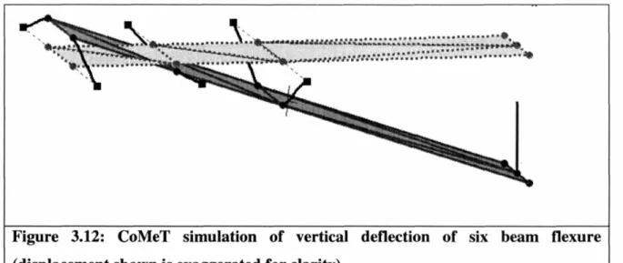
Figure 3.12: CoMeT simulation of vertical deflection of six beam flexure (displacement shown is exaggerated for clarity) ... 45

Figure 3.13: Groove flexure mounting ... 45

Figure 3.14: Grooved component with flexure grooves ... 46

Figure 3.15: Grooved component with probe mount ... 47

Figure 3.16: Balled component ... 48

Figure 3.17: Exploded view of Hybrid Positioning Fixture ... 48

Figure 4.1: Relationship between groove and ball center motion ... 50

(11)

Figure 4.2: HPF six-axis motion ... 50

Figure 4.3: Vector based model for in-plane motion ... 51

Figure 4.4: Global (CSo) and local (CSi) coordinate systems. ... 53

Figure 4.5: Out-of-plane motion - homed and displaced locations ... 54

Figure 4.6: Stiffness modeling... 56

Figure 4.7: HPF - Component breakup for stiffness modeling ... 57

Figure 4.8: Stiffness modeling steps ... 58

Figure 4.9: Forces acting on the HPF ... ... 59

Figure 4.10: Ball-groove contact schematic ... 61

Figure 4.11: Schematic of groove flexure ... 64

Figure 4.12: Groove flexure schematics ... 67

Figure 4.13: Six-beam flexure schematics... 68

Figure 4.14: Actuator-SBF connection ... ... 72

Figure 4.15: Unloading a spherical indenter (original figure by K.L. Johnson, Contact Mechanics [25]) ... 72

Figure 4.16: Contact forces and deflections for actuator-SBF connection ... 74

Figure 4.17: Coordinate systems used in transformation sequence ... 75

Figure 4.18: Coordinate transformation from ball-center to fixture centroid ... 77 11

(12)

Figure 5.1: HPF assem bled into test stand... 80

Figure 5.2: Hysteresis and creep of stack type piezoelectric actuator (figure from Tutorials: Displacement of Piezo Actuators [26]) ... 81

Figure 5.3: Sample strain gauge calibration chart ... 82

Figure 5.4: Actuator control scheme... 83

Figure 5.5: Six-axis displacement tests without fixture position feedback ... 85

Figure 5.6: Displacement tests (X, Y and Z) with position feedback ... 87

Figure 5.7: Displacement tests (0x, Oy and Oz) with position feedback ... 88

Figure 5.8: Linear parasitic error sources ... ... 89

Figure 5.9: Small displacement motion along Y axis and associated in-plane parasitics. 91 Figure 5.10: Repeatability tests at constant voltage... 94

Figure 5.11: CoMeT models of SBF ... 95

Figure 6.1: Finite element model - schematic... 99

Figure 6.2: Interface stresses for Poisson ratios v = 0.2 and 0.25 ... 100

Figure 6.3: Thin film buckling due to in-plane compressive stresses ar and ao ... 101

Figure 6.4: Radial tensile stress a, at edge (r = a) of coating surface (z = 0) ... 102

Figure 6.5: In-plane stresses at the coating surface and near center of contact ... 103

Figure 6.6: Normal stress (az) at center of contact (r = 0) on the coating surface ... 104 12

(13)

Figure 6.7: In-plane stresses a, and ao at the interface, in the coating ... 105

Figure 6.8: In-plane stresses a, and ae at the interface, in the substrate ... 106

Figure 6.9: Maximum tensile stress along interface (z = tc) ... 107

Figure 6.10: Shear stress along the interface for tc/a = 0.1 and 1.0 ... 108

Figure 6.11: Shear stress (r,) along interface for tc/a = 0.025 and 1.0 ... 109

Figure 6.12: Maximum shear stress (rz) along the interface ... 110

Figure 6.13: Tensile stress, ar, on coating surface (z --=0) at the edge of contact (r = a) 111 Figure 6.14: Maximum tensile stress, ar, along the coating-substrate interface ... 112

Figure 6.15: Maximum shear stress, r, at the interface ... 112

Figure 6.16: In-plane compressive stress ar and ae in the coating at r = 0 ... 113

Figure 6.17: Schematic of finite element model for interlayer analysis ... 116

Figure 6.18: Radial stress ar on the coating surface at the edge of contact (r = a) ... 117

Figure 6.19: Radial stress ar at coating-interlayer (Intl) and monolayer-substrate ... 118

Figure 6.20: Radial stress ar at interlayer-substrate (Int2) and monolayer-substrate ... 119

Figure 6.21: , along coating-interlayer (Intl) and monolayer-substrate interface ... 120

Figure 6.22: r, along interlayer-substrate (Int2) and monolayer-substrate interface ... 121

Figure 6.23: ar and ao in coating-interlayer (Intl) and monolayer-substrate interface... 122

Figure 6.24: ar and ao in interlayer-substrate (Int2) & monolayer-substrate interface ... 123

(14)

Figure 6.25: Tensile stress, ar, on the coating surface at the edge of contact (r = a) ... 125

Figure 6.26: Tensile stress, a,, at coating-interlayer and monolayer-substrate interface 126 Figure 6.27: Tensile stress, ar, at interlayer-substrate & monolayer-substrate interface 127 Figure 6.28: Shear stress r, along the coating-interlayer & monolayer-substrate ... 128

Figure 6.29: Shear stress r, along the interlayer-substrate & monolayer-substrate ... 129

Figure 6.30: ar and ae in coating-interlayer and monolayer-substrate interface ... 130

Figure 6.31: ar and ae in interlayer-substrate and monolayer-substrate interface ... 131

Figure A.1: Exploded view of Hybrid Positioning Fixture ... 143

Figure A.2: HPF - grooved component-base ... ... 144

Figure A.3: HPF - probe mount ... 145

Figure A.4: HPF - balled component-plate ... ... 146

Figure A.5: HPF - groove flexure ... 147

Figure A.6: Exploded view of test Stand ... 148

Figure B.1: Vector based model for in-plane motion ... 149

Figure B.2: Out-of-plane motion - homed and displaced locations ... 151

Figure B.3: Component of unit vector normal to displaced plane ... 152

Figure B.4: Excel worksheet - HPF kinematics ... 155

Figure D.1: Six-axis displacement test data (without fixture position feedback) ... 171 14

(15)

Figure D.2: Six-axis displacement test data (with fixture position feedback) ... 172

(16)

List of Tables

Table 1.1: Summary of key performance characteristics of the HPF ... 23

Table 2.1: State-of-the-art detachable fixtures and nano-positioning systems ... 29

Table 4.1: Validation of groove-flexure stiffness model ... 67

Table 4.2: Validation of the six-beam flexure stiffness model ... 71

Table 4.3: HPF stiffness - based on MATLABTM _{implementation of model ...} ₇₈

Table 5.1: Performance metrics and associated tests... ... ... 79

Table 5.2: Strain gauge calibration factors ... 83

Table 5.3 Standard deviation of fixture position (repeatability test) ... 92

Table 5.4: HPF stiffness - experimental vs. analytical results ... 95

Table 6.1: Comparison of FEA model and Hertz theory ... 99

Table 6.2: Stresses at the coating-substrate interface for v = 0.2 and 0.25 ... 100

Table 6.3: Analytic expression for stress in monolayer configuration ... 115

Table 6.4: Hard interlayer stresses compared to monolayer stresses ... 123

Table 6.5: Analytic expression for stress in hard interlayer configuration ... 124

Table 6.6: Soft interlayer stresses compared to monolayer stresses ... 131

Table 6.7: Analytic expression for stress in soft interlayer configuration ... 132 16

(17)

Chapter 1- Introduction

1.1 Motivation

The purpose of this research is to generate the knowledge required to design ultra-precision fixturing systems for nanometer-level accuracy and repeatability. This is important as maintaining acceptable costs and quality in many current and emerging products requires nanometer-level positioning and fixturing. For instance, the fields of photonics packaging, semiconductor test equipment, mask to wafer alignment and the like, require positioning in six axes with nanometer-level and micro-radian accuracy. In such applications, several parts might need to be positioned at many different machines, for instance in a manufacturing line. It is desirable that the fixturing system used to align and affix the part provide rapid, repeatable and accurate means to place and remove the parts. The stiffness and load capacity of fixtures are also important as these characteristics place limits on the fixture's accuracy and suitablility for various applications.

This work has focused on generating the knowledge engineers and scientists will need to design, fabricate and implement fixtures that satisfy the characteristics discussed above. Towards this end, this chapter will provide the reader with the background information required to understand the important characteristics of precision fixtures, nanomanipulators and the fundamental limitations that prevent the extension of current technologies to provide nanometer-level performance. A summary of the research approaches to addressing the fundamental limitations is also provided.

(18)

1.2 Precision fixture and positioning systems

1.2.1 Review of precision fixture technologies

A fixturing system or fixture provides means to locate or fix one component with respect to another. Numerous fixturing methods are utilized to achieve this. Typically they are passive and may be categorized into elastic-averaging and exact-constraint based methods. Elastic-averaging methods, for instance those shown in Figure 1.1, achieve precision by averaging errors over a large number of contact points. The averaging effect enables them to have high load capacity and stiffness. However they are by nature overconstrained, limiting their repeatability to about 5Jlm [1]. Here repeatability refers to the variation in position of the part over several cycles of placement and subsequent removal.

• ..

~;:I

RAIUSLOT DOVETAIL V/GROOVE

"/',.

COLLET

Figure 1.1: Elastically averaged alignment methods (figure by M.L. Culpepper,

Design and Application of Compliant Quasi-Kinematic Couplings [1])

On the other hand, exact constraint methods have number of constraints exactly equal to the number of degrees of freedom to be controlled. This makes the system deterministic and exact-constraint methods such as kinematic couplings, may provide sub-micron repeatability. Figure 1.2 shows two common configurations of kinematic couplings. As such, kinematic couplings have long been used in instrumentation design to provide economical means to locate components precisely [2]. These couplings date back to the 1800's, when Willis, Kelvin and Maxwell used them as fixtures in their experiments [3]. Kinematic couplings achieve precise positioning by providing six constraints or

(19)

small-area contacts to define the six degrees of freedom of the system.

(a) Three - groove (b) Tetrahedron-flat-vee (Kelvin clamp)

Figure 1.2: Kinematic couplings, C = constraint (adaptation of figure by L.C.

Hale, Principles and techniques for designing precision machines [4])

Much work has been done in formalizing the design process of these couplings [2,3]. Over the years these couplings and others, based on them, have been used in applications such as locating a chuck with respect to faceplate of a lathe [5], repeatable tool holders [6], locating parts onto machininig centers in an assembly line [7], Quasi-kinematic couplings for automotive assembly [1], two degree of freedom XY micro-stage [8], quick change industrial robot interface, modular high precision microscope [9] and the like. The principle limitations of traditional kinematic couplings were relatively low stiffness (compared to that of machine structure, approximately 50N/gm) and high contact stresses that limited their load capacity and life. These limitations were addressed through the use of high modulus ceramic materials and larger area contacts (canoe balls) [9]. Performance limitations resulting from contact friction have been partly addressed through the use of ceramic materials (repeatability approximately 0.3/Lm using SiN) [10] and more recently, by using low cost surface coatings [11]. More work is required to restrict friction-induced errors to below the nanometer-level. Incorporation of flexures within these coupling has also shown to reduce frictional hysteresis to 0.1/zm [12]. This work has not addressed the use of flexures to improve repeatability.

From the past work, we know that kinematic couplings and other passive fixtures may generally be designed to have the requisite stiffness and load capacity for most

(20)

instrumentation and manufacturing applications. Unfortunately, the accuracy of passive fixtures is strongly coupled to manufacturing and assembly tolerances. Here accuracy refers to the deviation of the average position of the part from the desired location. As a result, a passively fixtured system may be repeatable but not necessarily accurate. It is for this reason that passive positioning methods require either repeated calibration or ultra precision fabrication methods to minimize errors due to manufacturing and assembly of the fixture components. Additionally, thermal errors, which are time variable, cannot be addressed with the use of passive fixtures.

To address this limitation, fixtures incorporating actuators and mechanisms, are being developed to provide active correction capability. One such fixture is the ARKC (Accurate and Repeatable Kinematic Coupling) which has la repeatability of approximately 1.9,Lm/3.6/radian [13] and accuracy on the order of 1m/10,Lradian. This was a first step in providing accurate and repeatable fixtures, but the performance falls short of the nanometer-level goals of this work.

1.2.2 Review of generic positioning systems

Positioning systems that provide nanometer-level positioning, e.g. nanomanipulators, require active elements to sense and correct errors. The alignment elements of these machines are self-contained and therefore a locating interface is required to position parts with respect to the nanomanipulator. As such, these systems do not provide means to rapidly place and remove components. Each time a part is removed and then replaced on the positioning stage, its location may vary over several microns. Calibration is therefore required each time a part is attached to the manipulator. We must also consider that these systems use delicate machine elements, which limits system load capacity ( 20 - 50 N). Higher load capacities are needed to accommodate forces from weight of parts and from manufacturing and assembly operations. The stiffness of these systems is also low, resulting in low resonance frequencies and load induced errors. Due to the above discussed limitations, these systems are generally limited for use in low rate, low force

(21)

applications.

Fixturing and positioning systems contain between them the requisite characteristics for future fixturing-alignment equipment. In this work, we investigate the means to combine the desired characteristics while eliminating those characteristics, which make either method unsuitable for the task. As this work addresses both fixturing and positioning requirements, the system developed herein is called a Hybrid Positioning Fixture (HPF).

1.3 Hypothesis and research goals

In spite of the limitations mentioned earlier, kinematic couplings form a good starting point to develop the next generation of ultra-precision fixtures. Kinematic couplings have been shown to be repeatable to better than 300 nm [10]. They can also be easily and rapidly engaged and disengaged. Additionally, their stiffness and load capacity may be set to satisfy most instrumentation and manufacturing requirements. They only lack the capability to become accurate and repeatable at the nanometer level. The hypothesis of this work is that nanometer-level accuracy and repeatability may be achieved by:

1. By incorporating high resolution, high stiffness actuators and hysteresis free compliant mechanisms within traditional kinematic couplings, active fixtures capable of six-axis corrective motion with nanometer-level accuracy may be developed. 2. One of the factors limiting repeatability of traditional kinematic couplings is the

presence of friction at contact points. To achieve nanometer-level repeatability at reasonable costs, flexures may be incorporated to reduce frictional hysteresis at contact interfaces.

3. Additional performance improvement may be obtained through surface treatment of interfaces. This will promote the stability and longevity of the fixture contact geometry.

(22)

Toward this end, this work has the following research tasks/goals:

1. Integration of actuators and mechanisms: To achieve nanometer-level accuracy,

active error correction in six axes is required. This necessitates the generation of a fixture design with integrated actuators, mechanisms and sensors. A kinematic theory is needed to relate actuator commands to fixture position and orientation. It should also be noted that incorporating actuators and mechanisms would modify the fixture's stiffness characteristics. Thus, a stiffness model for the fixture is to be developed that would enable design optimizations to simultaneously achieve the desired stiffness and kinematic characteristics.

2. Integration of flexures at contact interface: Stick-slip at contacts in fixtures limits their repeatability. A main goal of this work is to design contact interfaces with integral flexures that prevent stick-slip. Flexure concepts are to be generated. Parametric models will be derived for the flexures and used to tune their stiffness so that they may prevent stick-slip.

3. Surface coatings: One means of improving repeatability and reducing fixture contact wear is to use hard surface coatings [11]. The design of coated interfaces for precision fixtures requires the knowledge of stresses in the coating, interface and substrate. Though much work has been done to understand the behavior of these stresses

[14,15], literature on stresses in thin coatings

{(t < 0.1) tc = coating thickness, a = contact radius} is not available. This class of

a

coatings <0.1 corresponds to typical coating configurations in practical fixturing applications. Design rules for thin coatings will be developed utilizing non-linear finite element analysis.

4. Experimental validation: The utility of new design concepts, the accuracy of engineering models, and the utility of the new design rules will be tested via experiments on a prototype Hybrid Positioning Fixture (HPF).

(23)

1.4 Hybrid Positioning -Fixture (HPF) Overview

This work has culminated in a new positioning device, the HPF. The prototype consists of the two parts as shown in Figure 1.3. The first part, shown in Figure 1.3 (a), is comprised of high-resolution piezoelectric actuators, flexural "V" grooves and compliant transmission mechanisms. The second part, shown in Figure 1.3 (b), consists of three l-inch diameter stainless-steel balls affixed to a plate. The test setup, shown in Figure 1.3 (c), was used to characterize repeatability, accuracy and stiffness of the HPF.

(a)Active component (b) Passive component (c) Test setup

Figure 1.3: Ultra-precision fixture prototype - Hybrid Positioning Fixture (HPF)

Table 1.1 summarizes the key characteristics of the HPF. The HPF has the potential to form the basis for the design of fixtures for the next generation of instrumentation, ultra-precision and nano-manufacturing processes.

Table 1.1: Summary of key performance characteristics of the HPF

Axes Range Accuracy Repeatability Stiffness

Open loop Closed loop (N/J.lm)

6 _50J.lm

_&

100nm

&

5nm 100 nm

&

7

625 flradians 2J.lradians 2J.lradians

An important application of the HPF is in palletized manufacturing. Figure 1.4 shows an example of a palletized system. Balled pallets are marked with passive identifiers (bar code or RFID tag) characterizing their systematic error sets (SES). A systematic error set

(24)

is a data set that contains all systematic errors for the balled pallet. Such errors would include manufacturing and assembly errors. The SES is obtained via calibration exercises. Each machining station is equipped with the active grooved component and the SES of the machine. When a fixture is engaged, the machining station reads the SES of the balled component and uses models to determine how the active elements should be commanded in order to achieve a desired fixture position and orientation.

~=

Pallet

@=HPF

Figure 1.4: Integration of the HPF into a palletized machining process

1.5 Thesis overview

This thesis covers the modeling, design and characterization of the Hybrid Positioning Fixture. Chapter 2 presents the state-of-the art in detachable fixtures and other competing technologies. Chapter 3 covers the design of the HPF. Chapter 4 details the analytical models of the fixture's kinematics and stiffness. Chapter 5 presents the experimental performance characterization. Chapter 6 covers non-linear finite element analysis of thin coatings and design guidelines for the use of thin coatings in precision fixtures. Chapter 7 presents the conclusions, a summary of the fundamental contributions of the work and potential topics of future work.

(25)

Chapter 2 - State-of-the-art

This chapter presents the state-of-the-art in active fixtures and a comparison of these fixtures with nano-positioning systems.

2.1 Active precision fixtures

Much research on precision fixtures has been focused on passive fixtures, mainly kinematic couplings. These fixturing systems are limited to micron-level accuracy and repeatability, and are therefore not suited for next generation nano-manufacturing and ultra-precision applications. The Hybrid Positioning Fixture (HPF) with its nanometer-level accuracy and repeatability meets this need. It is important to understand the prior art in active precision fixtures before one can appreciate the advances embodied in the HPF. Toward this end, two active fixtures are presented in the subsequent sections. These systems are representative of the state-of-the-art prior to this work.

2.1.1 Precision X-Y micro-stage

Figure 2.1 shows a micro-positioning system developed by Taylor J.B. and Tu J.F [8]. The stage consists of a base plate with three "V" grooves placed 1200 apart. The upper plate contains three spheres that mate with the "V" grooves in the base plate. One of the spheres is rigidly fixed while the remaining two may be maneuvered within their respective slots using linear actuators. The part to be positioned is connected to the upper plate at the point C shown in Figure 2.1 (b). The position of point C is of interest here and is controlled by motion of the actuators. The micro-positioning stage was shown to have a resolution of lnm over a range of 40 x 40mm. The authors suggest the use of such systems in light load applications such as microelectronics particularly in a transfer line environment where the detachable and repeatable nature of the fixture is an automatic advantage.

(26)

(a) X-Y micro-stage schematic (b) Geometric model of X- Y stage

Figure 2.1: X-V micro-stage with maneuverable kinematic coupling mechanism (figure by J.B Taylor and J.F Tu, Precision X-V micro-stage with maneuverable kinematic coupling mechanism [8])

However, the system has the following limitations:

1. Its performance is not adequate for applications requiring nanometer-level accuracy. In these applications, positioning methods with resolution of about O.lJ.lm are utilized

[8].

2. The in-plane motion of the stage is highly coupled and the system cannot position in any given position and orientation on the XY plane. The authors propose to address this problem through use of an additional linear actuator for the third sphere. Even with the modification, the system is limited to having three degrees of freedom. This implies that the system cannot compensate for out-of-plane errors.

2.1.2 Accurate and repeatable kinematic coupling (ARKC)

In 2003, the accurate and repeatable kinematic coupling was developed at the PCSL MIT [13,16]. The ARKC is shown in Figure 2.2. It combines the repeatability of traditional kinematic couplings with six-axis adjustment to attain micron-level accuracy and repeatability. This system addressed the limited degree of freedom of the XY micro-stage. The ARKC consists of two components; the active component consisting of three

(27)

dual-axis stepper motors and a passive component consisting of three "V" grooves. Each actuator shaft is connected to a ball such that the shaft axis is offset from the ball-center. Rotation of the shafts causes in-plane motion of the balled component whereas linear translation of the shafts causes out-of-plane motion. Thus, correction in six axes is possible. The ARKC has a measured la repeatability of approximately 1.9jlm/3.6jlradian [13] and open loop accuracy on the order of approximatelyljlm/l0jlradian.

(a) Component with actuators and balls (b) Component with grooves

Figure 2.2: Accurate and Repeatable Kinematic Coupling (figure by M.L

Culpepper, et al., Design of integrated mechanisms and exact constraint fixtures for micron-level repeatability and accuracy [13])

Though the ARKC has a range of applications in photonics and automotive industry, nanometer-level accuracy and repeatability were elusive due to hysteresis associated with use of rolling element bearings, stick-slip at contact interlaces and resolution of stepper motors. These limitations are addressed by the present work.

2.2 Competing technology - Nano-positioning stages

Nano-positioning stages are used in a wide range of applications including photonics packaging, semiconductor test equipment, precision mask and wafer alignment, scanning interlerometry, biotechnology, micromanipulation and the like [17]. These positioning stages are capable of nanometer-level accuracy. These systems would be close competitors of active fixturing systems if they could provide easy means to place and remove parts on the stage, or in other words, provide mate-unmate capability.

(28)

Many state-of-the-art nano-positioning systems utilize piezoelectric driven flexure stages to achieve nanometer-level accuracy and resolution. Piezoelectric actuators in combination with closed loop control can provide sub-nanometer-Ievel resolution and accuracy. Additionally, flexures may be used to achieve hysteresis free motion transmission. The HPF utilizes both flexures and piezoelectric acuators to achieve nanometer-level positioning [18].

Commercial nano-positioners include both serial and parallel kinematic stages. Figure 2.3 shows a schematic of serial and parallel kinematic, nano-positioning stages .. Serial kinematic stages have several limitations including higher inertia, high center of gravity, inability to correct for off-axis errors and moving cables that are the source of compliance and vibration errors. Thus parallel kinematic stages are best suited for nano-positioning applications [18].The HPF has a parallel kinematic architechture that avoids the limitations of serial stages.

(a) stacked serial kinematic 2-DOF stage (a) Monolithic parallel 3-DOF stage

Figure 2.3: Serial vs. parallel kinematic naDo-positioning stages (figure from

(29)

Table 2.1 compares the performance of the detachable fixtures including HPF and state-of-the-art nano-positioners from Physik Instrumente.

The HPF matches the performance of the best nano-positioners in terms of motion capability (axes), resolution and natural frequency. Additional advantages of the HPF include:

1. The HPF has about 10 times larger load capacity than the state-of-the-art nano-positioning systems.

2. The HPF is amenable to use in large scale applications as part of the assembly or transfer line. This is due to the ease with which the fixture may engage-disenage and yet retain nanometer-level repeatability.

3. The "drop and forget" capability makes integration into automated production/testing lines easy. The part to be positioned may be attached to the passive balled component (pallet) and the active grooved component may be fixed to the machining or testing center. A robotic arm may pick up the part (attached to the pallet) and place it roughly over the grooved component. The balled component automatically aligns to the

29

Table 2.1: State-of-the-art detachable fixtures and nano-positioning systems

Axes Resolution Accuracy Repetability Stiffness Load Natural (pmg/prad) (plm/prad la (n/prad) (N/pm) capacity freq (Hz)

~~~~) I ~[N] XY [8,16] 2 1/- 1/- 400/- 150 4000 unknown stage ARKC 6 1/10 1/10 2/4 150 4000 unknown [16] HPF 6 0.003/- 0.1/2*** 0.1/2 10 450 202**

P-762 [19] 5 0.01/0.5 unknown N/A unknown 20 200**

P-587 [17] 6 0.008/0.1* unknown N/A unknown 50 103**

*Closed loop operation **In-plane XY

(30)

correct position on the grooved component. This is termed as "drop and forget," meaning that the balled component is droped on to the grooved component without assessing the subseqent alignment accuracy. The kinematics of the HPF ensures that it attains the correct position. This is shown schematically in Figure 2.4.

Balled component

Pick part Drop Automatic alignment

(31)

Chapter 3 - Design of the HPF

This chapter focuses on the concepts and system-level design choices, which were made in designing the prototype Hybrid Positioning Fixture. The goal of this chapter is to provide a discussion that outlines the thought process, which drove the decisions made in

setting up the architecture of the HPF. When appropriate, quantitative data is provided, although sound engineering knowledge/experience is also used to decide on the best embodiment of a sub-system or system design. Subsequent chapters will provide

assessment and application of quantitative analyses.

The chapter is organized into three sections. The first section discusses the fundamental issues associated with designing precision fixtures for nanometer-level accuracy. The

second section discusses the conceptual design, while the third section details the design of the individual components. Detailed component drawings are available in Appendix A.

3.1 Fundamental issues

3.1.1 Exact constraint design

The fundamental principle of designing precision fixturing systems is the provision of exact constraint. In order to determinstically locate a rigid body in three dimensional space, six constraints are required. If the fixturing system provides exactly six constraints, the location of component is uniquely determined. This makes the fixture performance predictable and enables closed-form modeling, thereby reducing engineering costs

associated with design iterations [20]. Provision of extra constraint or "over constraint" of the system will often lead to parts binding together or parts being too loose. As a result, the relative position of these parts is not well defined. Figure 3.1 shows schematically the

constrast between exact constraint and over constraint.

(32)

C I I Tinh I DraIrni Ifeo / I II C I I

l____

10_

A

I I I WJJ/

C

(--I I ¥ _I _

(a) Over constraint - Loose (b) Over constraint - Tight (c) Exact constraint

Figure 3.1: Over constraint vs. exact constraint (figure by D.L. Blanding, Exact Constraint: Machine Design Using Kinematic Principles [21])

"Elastic-averaging" based alignment methods, use the averaging effect of competition between "extra" constraints to obtain high stiffness, load capacity and moderate repeatability. These methods are not well-suited (repeatability limited to approximately 5pm) for emerging precision alignment needs due to problems associated with over constraint.

3.1.2 Repeatability vs. Accuracy

The two primary issues in the design of precision fixtures are "repeatability" and "accuracy".

"Precision (of position), also called repeatability, is the degree to which a part or a feature on a part, will return to exactly the same position time after time." [21]

"Accuracy (of position) is the degree to which location of a part or feature exactly coincides with its desired or intended location." [21]

These concepts are illustrated schematically in Figure 3.2, wherein a ball is constrained within a "V" shaped groove. Figure 3.2 shows how exact constraints may be employed to insure that the ball returns to the same position (with a small spread) even after repeated engagement-disengagement sequences. This indicates that the system is "repeatable" and its repeatability is given by the variation in relative location (r). Figure 3.2 also shows

(33)

that, even with a small spread, the system could still be far from the desired location. In other words, it is not "accurate" and its accuracy (a) is given by difference in actual and desired positions. Typically, repeatability may be achieved independent of accuracy, as is done in kinematic couplings. Accuracy on the other hand, depends on factors such as manufacturing and assembly tolerances, and time variable error sources such as external loads and thermal effects.

3.1.3 Friction and wear

The repeatability of kinematic couplings is limited by friction and wear of contact interfaces. The effect of friction on repeatability may be estimated using Equation 3.1 [22].

f 2 1/3 2/3

k

3R

E

(3.1)

Where:

R = equivalent radius of curvature E = equivalent Young's modulus

P = external load

/ = coefficient of friction.

33

Desired

Actual

Accuracy

Repeatability

C

=

Constraint and a

(34)

The frictional force acts on the compliance of the contact interface to pull the fixture off position. The estimate is obtained as a product of frictional force (f= uP) and compliance (1/k) of a single Hertzian contact under load P.

The magnitude of non-repeatable errors associated with friction-induced stick slip and wear may be reduced by:

1. Increasing contact stiffness or modulus (E) 2. Decreasing coefficient of friction (u) 3. Minimizing contact damage and wear

4. Minimizing relative motion between ball and groove

With the use of specialized ceramic materials for the ball-groove interface, positioning repeatability of about 300nm has been achieved [10]. The high stiffness, wear resistance and low friction coefficient of the ceramic materials endows them with excellent performance capability. However, custom coupling components made from ceramic materials are difficult and expensive to manufacture. With these considerations, hard-coated ball-groove surfaces are to be explored as a cost-effective alternative to high-cost ceramic components [11]. Frictional hysteresis, a component of non-repeatability, is theoretically zero if there is no relative motion at the contact interfaces. By increasing compliance in direction parallel to that of the relative motion, hysteresis may be reduced

[12].

3.1.4 Active vs. passive fixtures

Though repeatable, the accuracy of passive fixtures is strongly coupled to manufacturing and assembly tolerances. To overcome these limitations, actuators and mechanisms must be integrated within the fixture so that they may be utilized to provide active correction capability. Figure 3.3(a) shows the limitation imposed on the accuracy of a passive fixture due to manufacturing errors. Figure 3.3(b) shows the improved accuracy which may be obtained by incorporating an active element (actuator = A) within the fixture. The

(35)

mated position in (a) is "actuated" to obtain the more accurate position shown in (b).

Motion of ball center (b) Active fixture

(a) Passive fixture

Figure 3.3: Active vs. passive fixture

3.2 Conceptual design

,-I I I

,

\

,\

0~\~

3.2.1 Design for nanometer-level accuracy

To actively compensate for errors, actuators and mechanisms, which are integrated into the fixture should be able to work together to provide error correction in six-axes. We can gain insight into how this is best accomplished by examining the mechanism nature of kinematic couplings. A kinematic coupling's six-constraints are analogous to the constraints in a Stewart platform. This is shown schematically in Figure 3.4. Stewart platforms generate motion by changing the constraints on the platform, therefore it should be possible to adjust a kinematic coupling's position and/or orientation by adjusting the location of the constraining elements (balls and/or grooves) [13].

(36)

Groove far-field points

..

+

.

-f..

.

_.

...

+

...

+

(a) Two constraints at a ball-groove interface (b) Six constraints in a kinematic fixture Figure 3.4: Analogy between a kinematic fixture and a Stewart platform (figure by M.L Culpepper, et al., Design of integrated mechanisms and exact constraint fixtures for micron-level repeatability and accuracy [13])

Two concepts, which have been used to achieve six-axis adjustment were presented in [13] and are shown in Figure 3.5.

»j j+--e

(a) Linear groove motion concept (b) Eccentric ball-shaft concept

Figure 3.5: Concepts for achieving six-axes correction (figure by M.L Culpepper, et al., Design of integrated mechanisms and exact constraint fixtures for micron-level

(37)

In concept (a), the component to be positioned is mounted on the balled part of the fixture while the grooved part, containing the active elements, is fixed to the ground. This concept utilizes six linear actuators to move the groove surfaces and hence the balled component. Concept (b), on which the ARKC is based, consists of three balls mounted on eccentric shafts connected to dual-axis stepper motors. Rotation of the shafts causes in-plane motion of the balled component whereas linear translation of the shafts causes out-of-plane motion. Rolling element bearings are utilized to permit rotation and translation of the ball-shaft sub-assemblies. In this design, the part to be positioned is connected to the grooved component while the balled component is fixed to the ground.

Concept (a) was chosen for the HPF since it is amenable to implementation with piezoelectric actuators and flexural bearings. The hysteresis free nature of flexure bearings and sub-nanometer resolution of the piezoelectric actuators may be used to avoid the limitations imposed by the rolling element bearings (friction) used in the alternate design. Thus, nanometer-level accuracy may be achieved. The kinematics of the HPF is discussed in more detail in Section 4.1.

3.2.2 Design for nanometer-level repeatability

In a traditional "V" groove, as the ball mates with the "V" groove the interface is compressed elastically. This compression is accompanied by a tangential motion of the contact point, in conformance to the constraints. The tangential motion leads to macro slip at the contact interface and lends uncertainty to the position of the contact point and hence the ball center. This uncertainty is termed as hysteresis. Figure 3.6 depicts this process schematically.

(38)

Figure 3.7 presents results from [12], which shows the hysteresis associated with loading and unloading of a kinematic coupling. This hysteresis is the difference between compression of the contact as the preload increases and as the preload decreases. Figure 3.7 (a) shows that for a coupling with flexure grooves the hysteresis is reduced by a factor of 10, compared to traditional grooves. Figure 3.7(b) shows flexure hinges cut into groove surfaces; the flexure has relatively high compliance, Ct, tangential to the surface and low compliance, C,, normal to the surface. The low tangential compliance permits the ball to adjust in the groove without causing relative motion between the ball and groove surfaces. The preload on the coupling is cycled without disengaging the balled and grooved components. Hence, the effect on repeatability over several cycles of engagement and disengagement of the coupling components is uncertain. As a result, the potential for this design concept to eliminate the effects of stick slip (this is not hysteresis) and hysteresis, which result from the engaging-disengaging of the contacts, is uncertain. As both sources of error must be addressed to obtain nanometer-level accuracy, the subsequent sections will focus on the design of flexures that address these errors.

(39)

Flu 1000 o500o I COmAndW V-rgmo 2 8elln.__, VFoagw V. I - I _-J 1

,II

/

//

/

/4,.

it

/

,/

Li

2 1 4 - a, ml

(a) Measurements of preload force Fp and elastic deflection 6,p

/

n 2a

(b) Ball in V-groove with elastic hinges

Figure 3.7: Measurements of preload force F, and elastic deflection Jp (figure by C.H. Schouten, et al., Design of a kinematic coupling for precision applications [12])

In designing the flexure, high stiffness in direction normal to interface is desirable, with regard to both repeatability and overall stiffness of the fixture. On the other hand, high compliance in the tangential direction is required to minimize relative motion. However, reduction in tangential stiffness also reduces overall stiffness of the fixture. In a conventional ball-groove contact the ratio of tangential to normal contact stiffness is approximately 0.83. This implies that the tangential stiffness is nearly equal to the normal stiffness. To achieve a balance between fixture stiffness and reduction of sliding motion between the contacts, the design requirement for the groove flexure was chosen to be

Kt < 10 Kn Where: Kt = Tangential stiffness Kn= Normal stiffness 39

7 I/

I II or I I 1 · I

(40)

3.3 Component design

The HPF consists of two major components: the grooved component and the balled component. The grooved component, incorporates the actuators, bearings, and groove flexures. This part is analogous to the component containing "V" grooves in a traditional, three-groove kinematic coupling. The balled component contains three balls that are press fitted into a plate. This component is identical to the balled component of a three-groove kinematic coupling. Sections 3.3.1 to 3.3.5 describe elements of the grooved component and while Section 3.3.6 describes the balled component.

3.3.1 Actuators

Several actuators were considered for the design, including electromagnetic, lead-screw-stepper motor combinations, however piezoelectric actuators were the only type capable of delivering tens of microns stiffness and nanometer-level resolution. PA50-14 SG (stack type) piezoelectric actuators supplied by piezosystem jena Inc., are used in the prototype. The key characteristics of the piezoelectric actuators used in the design and testing of the HPF are listed below [23]:

* Input voltage (-)15 to (+)100 V * Range - 50pm

* Resolution - 0.07nm

* Stiffness- 20 N/mn * Load capacity - 1000 N

* Integrated strain gauge for displacement measurement * Maximum tensile loads approximatelyl50N

3.3.2 Flexure bearings

In the present application, traditional linear bearings cannot be utilized to transmit motion of the actuator to the groove surfaces due to stick slip between the bearings and their races. This limitation does not exist for flexure bearings, which utilize elastic deformation

(41)

to achieve motion. When the flexure bearing is placed in series with the actuator, the stiffness of bearings in the direction of actuator motion should be small, e.g. less than 0.1 of the actuators stiffness. This ensures that the actuator range is not reduced by more than 10%. It is also important for the flexure bearing to possess high stiffness in other directions. This helps to reduce parasitic errors and errors due to loads that act in directions other than the actuation direction, e.g. preload error loads or o~her external disturbance forces. The six-beam flexure design (SBF), shown in Figure 3.8, was chosen to guide the motion of the piezoelectric actuator. Although the design could have used four, eight or more flexure beams, it was found that six beams would provide the requisite compliance in the actuation direction and high stiffness in other directions. The motion of the bearing is small enough, (about 50 ~m) that stiffening effects in the beams may be neglected. Detailed stiffness characteristics of the groove flexure are presented in Section 4.2.4.

SBF

Figure 3.8: Six beam flexure

3.3.3 Actuator mounting

The stack type piezoelectric actuators used in the HPF are primarily "push" type and the mounting must be designed to eliminate any tensile or torsion loads. The mounting method consists of a ball mounted to the tip of the actuator, which engages a "V" -groove on the SBF. This provides constraint in two directions while eliminating torsion loads on the actuator tip. Additional constraints are provided by the actuator clamps and the flat face supporting the back of the actuator. Figure 3.9 shows the grooved component with

(42)

the actuators and six beam flexures.

(43)

1.1.1 Groove flexure

Different concepts were considered for the groove flexures and are shown in Figure 3.1.

Concepts (a) (b) (c)

Achieving tangential compliance -1 -3 0

Modeling complexity -1 2 0

Error / parasitic motion 0 -3 0

Total -2 -4 0

Figure 3.1: Groove flexure concepts

The concepts were compared based on:

1. Ease of achievine desired taneential stiffness for a eiven flexure size: Concept (a)

is assigned a negative value due to the difficulty in packaging the flexural spring elements to achieve the desired tangential compliance. Concept (b) is assigned a higher negative value due to the relative manufacturing complexity and the large flexure height or thin neck size that is required.

2. Modeline: As we wish to develop an analytic stiffness model for the fixture, the

flexure concept should be amenable to parametric modeling. Concept (a) is assigned a negative value due to relative complexity of modeling the spring elements. For concept (b), analytical models are readily available in literature. Concept (c) is composed of simple beam elements and is therefore easier to model and manufacture than concept (a).

3. Parasitic errors: The flexure-associated motions of the groove flexure in directions

normal and tangential to the groove's contact surface should be decoupled to enable independent stiffness tuning. This is expressed as error or parasitic motion, which implies motion in a direction(s) leading to undesired motion in another. With respect

(44)

to this parameter, concept (b) has relatively large susceptibility for parasitic motion. Rotation about the center of the necked portion leads to undesired motion normal to the flexure surface.

Based on the concept comparison shown in Figure 3.10, concept (c) was chosen as the best concept. The final design of the groove flexure is shown in Figure 3.11. The groove flexures were manufactured using 6061 Aluminum, with a 316 stainless steel plate bonded to the surface that forms the contact surface. These groove plates may easily be replaced with other materials if required.

Kt < 0.1 Kn

Kt

=

2.1 N/J.lm

Kn

=

34 N/J.lm

w

= width

t

= thickness

Figure 3.11: Groove flexure - final design

3.3.5 Groove flexure mounting

With regard to mounting the groove flexure on the six-beam flexure, the challenge is to minimize vertical deflection of the flexure resulting from the applied preload. Figure 3.12 shows a CoMeT simulation [24] of the flexure's deflection under a vertical load.

(45)

Figure 3.12: CoMeT simulation of vertical deflection of six beam flexure (displacement shown is exaggerated for clarity)

The normal force on the groove surface may be decomposed into components Fz and Fy as shown in Figure 3.13. These force components result in moment Mx about the X- axis of the SBF and is given by Equation 3.2.

Triangular mount

y

Lgf

sina/2

b

... ~

SBF

Lgt cosaj2

Figure 3.13: Groove flexure mounting

Mx =FX*( Wgf cosa+ Lgf ;ina + ; J-FY*(b+ Lgf ;osa +wgf sina

J

(46)

By appropriately selecting the dimension b, the moment Mx may be balanced to minimize the twist and thereby the deflection of the flexure. Equation 3.3 gives the required dimension b.

For Mx =0, from Equation 3.2

(Wgf cosa+ Lgf ₂sina +W)sina₂ ( _Lgf _cosa _. )

b= --- - ----+ Wgf SIna

cosa 2

L_gf(sin2 a-cos2 a) wtana => b

=---+---2cosa 2

(3.3)

For a groove angle (a) of 60° b

=

Lgf +w..f3 results in Mx = 0, thereby minimizing the

2 2

vertical deflection of the flexure. Figure 3.14 shows the complete grooved component with all the sub-elements, namely the actuators, flexure bearings (SBF) and the groove flexures.

(47)

3.3.6 Capacitance probe mount

To monitor the position of the fixture's balled component in six axes, a minimum of six probes are needed. Three of these probes are mounted on the test setup and are used to measure the in-plane motion. For further details, see Section 5.2. Three other probes, which are mounted on the grooved component, measure the out-of-plane motion of the balled component. Figure 3.15 shows the probe mount, which is attached to the grooved component and used to hold the out-of-plane sensors.

Figure 3.15: Grooved component with probe mount

3.3.7 Balled component

The balled component consists of three 316 stainless steel balls, pressed into sleeves that are in turn pressed into an aluminum plate. The sleeves are utilized instead of directly pressing the balls into the plate, to avoid interference with the groove flexures. The sleeves themselves consist of a smaller sleeve fitted into a bigger sleeve. The height of the smaller sleeve is designed such that a little more than half of the ball is within the sleeve. Figure 3.16 shows the balled component and a cross sectional view of the sleeves.

(48)

(a) Balled component

Figure 3.16: Balled component

Outer sleeve

Inner sleeve (b) cross sectional view of sleeve

Figure 3.17 shows an exploded view of the Hybrid Positioning Fixture.

Balled component - plate

/

Balls Groove plate ~

0

0 ~O>

',0

0 <>

\,

~

'0

\

~ ~~ !1 ~

·

Cylindricalball mount

~J,~

'probe mount

~~

0,

Grooveflexure ~ '+-Clamps , Piezoelectric Actuators

,

Grooved component - Base Figure 3.17: Exploded view of Hybrid Positioning Fixture

(49)

Chapter 4 - Analytic modeling

The chapter is organized into two segments. The first segment covers the kinematic modeling of the HPF and the second segment describes stiffness modeling. The former, deals with modeling the forward and inverse kinematics that define the relationship between motion of the actuators and that of the HPF. The later, gives a relationship between the external forces applied to the fixture and the resulting deflections, which

must be added to the kinematic analysis to capture the true position of the HPF.

4.1 Kinematic modeling

4.1.1 Overview

To achieve improved accuracy, active correction in six axes is required. This requires a deterministic kinematic model of the system that relates input from the active element (actuator) to the motion of the fixture. Common terminologies used in this regard are "forward kinematics" that determines the motion of the system resulting from a given set of actuator inputs and "inverse kinematics" that determines the actuator inputs required for a desired motion of the fixture.

The part to be positioned is connected to the balled-component. Therefore, in developing the kinematics of the fixture, we are interested in studying the motion of the balled-component's coupling centroid. The position of the balled-component is defined by position of the three ball centers. The basic principle, behind the adjustable kinematics of the HPF is that the motion of the groove surfaces leads to motion of the corresponding ball centers. This is demonstrated schematically in Figure 4.1. Equations 4.1-4.2 describe this relationship mathematically. Here the inward motion (towards the ball center) of the grooves is considered positive since it corresponds to the positive displacement of the actuators.

(50)

,-I , I fl911

+:

I I I 1-l1z₁ -, I I I - +flgl2 I I I _I I-I I I flgl1

+i

I I I '--Az1 -I I I I +flgl2 I I , ..J

(a) In-plane motion of ball center (b) Out-of-plane motion of ball center

Figure 4.1: Relationship between groove and ball center motion

~g'1-~g'2

~y'= I I

I 2 (4.1)

(4.2)

The six-axis motion of the HPF is achieved by a combination of motions of the groove surfaces. Examples of the HPF's motion are provided in Figure 4.2.

(a) 8X translation (b) 8Y translation (c)

ez

rotation

(a)

ex

rotation (b)

ey

rotation (c) 8Z translation

(51)

4.1.2 In-plane motion

Figure 4.3 depicts two configurations of the coupling. One, wherein the balled component coincides and the other where it is displaced with respect to the coordinate system CSo attached to the grooved component.

The solution to the in-plane kinematics is based on vector loops projected in the plane of the coupling. The vector loops share between them the centroidal displacement

rA = Xc.i + Yc.j . Three vector loops may be written corresponding to each ball-groove

mate, to obtain Equation 4.3.

rI + rl - rl = rA r2 + rA2 - r2= rA r3 + r3 - r3'= ra Where: rq = Xq i + Yq - j+ Zq k (4.3) (4.4) 51

mr

3

Xm

_ _ _ _ _ _ _ _ _ _

(52)

This method of vector loops is similar to that utilized in [13]. These equations may then be expanded to obtain relationship between displacement of the ball centers and balled-component's centroid. In developing these equations, small angle approximations have been made (assuming Ozc < 1000 pradians) - sin(Ozc) Ozc and cos(Zc) = 1.

x3+ Ax3 1 Y3 +AY3 = zc Z3 + AZ3 1 0 O -6Z 1 0 0 O XC L.c[ 1] 0 YC L.s[61 1] 1 0 0 0 1 1 L2 .c[2] 2 [62021 0 1

L

3

.c[

0

31]

L3 s[63] (4.5)

1

X =AX + (Lt.s[61 ].(Ay2-Ayl)

L2.c[92]- L.¢[1] Y = Ay2-_ L2.c[62]. (Ay2- Ayl) ) 6 = vY2 - AY₁ .4L 2.c[64-L.c[9] (4.6 (4.7) (4.8)

Where ri = x + yJ, r i = (x + Ax)' + (y + Ay) , Ozc is rotation about Z-axis and L= IrI .

Figure 4.4 shows the coordinate systems attached to the grooved component. The global coordinate system CSo is attached to centroid of the component and three local coordinate systems CS's are placed at the vertices corresponding to the ball-groove mates. Equation 4.9 defines the transformation between the global (CSo) and the local (CSi) coordinate systems.

Xi-

-Ci[i]

-A]

Yi = [il] C[0i] Zi O 0 1 Csi iO O

0 xio0

0 0 Yio 1 0 Zio o 1L 1 CSO xI + Ax1 Yl + AY1 Z1 + AZ 1 X2+ AX2 Y2 + AY2 Z2 + Az2 1 (4.9)