Design of versatile and low-cost shaft sensor for health monitoring

Design of Versatile and Low-Cost Shaft Sensor for

Health Monitoring

by

Erik M. Gest

FEB 252019

LIBRARIES

ARCHIVES

B.S., Massachusetts Institute of Technology (2017)

Submitted to the Department of Mechanical Engineering

in partial fulfillment of the requirements for the degree of

Master of Science in Mechanical Engineering

at the

MASSACHUSETTS INSTITUTE OF TECHNOLOGY

February 2019

Massachusetts Institute of Technology 2019. All rights reserved.

Signature redacted

A uth or ...

....

Department of Mechanical Engineering

January 22, 2019

Certified by ...

Signature redacted

I

7,

Kamal Youcef-Toumi

Professor

Signature redacted

Thesis Supervisor

Accepted by. .

Nicolas Hadjiconstantinou

Graduate Officer, Department of Mechanical Engineering

[I

Design of Versatile and Low-Cost Shaft Sensor for Health

Monitoring

by

Erik M. Gest

Submitted to the Department of Mechanical Engineering on January 22, 2019, in partial fulfillment of the

requirements for the degree of

Master of Science in Mechanical Engineering

Abstract

Virtually every mechanized form of transportation, power generation system, indus-trial equipment, and robotic system has rotating shafts. As the shaft is often the main means of mechanical power transmission, measuring the torque, speed, vibra-tion, and bending of the shaft can be used in many cases to access device performance and health and to implement controls. This thesis proposes a shaft sensor that mea-sures all of these phenomena with reasonable accuracy while having a low cost and simple installation process. This sensor transfers strain from the shaft and amplifies it to increase sensitivity. Furthermore, this sensor requires no components to be in the stationary reference frame, allowing the entire device to rotate with the shaft. A pro-totype is presented. Experimental results illustrate the effectiveness of the proposed system.

Thesis Supervisor: Kamal Youcef-Toumi Title: Professor

Acknowledgments

First and foremost I would like to thank my family: Mom, Dad, Daniel, Sarah, and Luke. My education would not have been possible without them and I owe everything I've accomplished to them. Thank you for the Skype meetings, care-packages, and support.

I would also like to thank Japan Steel Works, our project's sponsor. Their financial and technical help was invaluable to the project. I would like to specifically thank Mikio Furokawa and Takayuki Hirano for their assistance.

Furthermore, I would like to thank my fellow lab-mates in the Mechatronics Re-search Laboratory. Thank you for helping keep my days bright and for all the advice to further my research. It was a pleasure working with you.

Last but not least I would like to thank my advisor Professor Kamal Youcef-Toumi. You are one of the most genuinely caring people I have ever met and your constant support of the students you advise is incredible. I cannot imagine having a better advisor.

Contents

1 Background

1.1 Health Monitoring .

1.2 The Internet of Things . . . 1.3 Novel Sensor . . . . 1.4 Primary Application . . . .

2 Benchtop System

2.1 Background . . . . 2.2 Design . . . .

3 Torque and Bending Sensor

3.1 Background . . . . 3.2 D esign . . . . 3.2.1 Torque Calculations . . . . . 3.2.2 Bending . . . . 3.2.3 Instrumentation . . . . 3.2.4 Construction . . . . 3.3 Results . . . .. . . . . 3.3.1 Stationary vs. Rotating Shafts 3.3.2 Stationary Results . . . . 3.3.3 Rotating and Bending Results

3.3.4 Long Term Drift . . . .

17 17 18 19 19 21 21 21 27 27 29 30 34 34 37 40 40 40 41 44

. . . .

. . . .

. . . .

. . . .

. . . .

. . . .

4 Acceleration 53 4.1 T heory . . . . . 53 4.2 Selection . . . . 57 4.3 R esults . . . . 58 5 Power Generation 61 5.1 Requirements . . . . 61 5.2 Background . . . . 62 5.3 Brushless Generator . . . . 64 5.3.1 O verview . . . . 64

5.3.2 Static Mechanical Model . . . . 65

5.3.3 Dynamic Mechanical Model . . . . 68

5.3.4 Implementation . . . . 69 5.3.5 Results . . . .. ... 69 6 System Integration 73 6.1 M icrophone . . . . 75 6.2 Wireless Communications . . . . 76 7 Conclusion 79 7.1 Sum m ary . . . . 79 7.2 Future Work . . . .. . . . . 79 A Engineering Drawings 81 B Wiring Diagrams 87 C Operational Code 89 C.1 Sensor Code (C++) . . . . 89

C.2 Receiver Code (Python 3.6) . . . . 93

C.3 Benchtop Arduino Code (C++) . . . . 94

C.4 PWM Shift Code (C++) . . . . 98

D Analysis Code

D.1 Data Processing Code (Python 3.6) . . . . D.2 View Results Code (MATLAB) . . . . D.3 FFT of Torque Signal Code (MATLAB)

D.4 Acceleration Simulation Code (MATLAB)

D.4.1 AccelMethods.m ...

D.4.2 plotSpeedsFromSignals.m . . . . .

E Bills of Materials

F Finite Element Analysis Details

G Instructions for Fabrication, Mounting, and Testing G.1 Sensor Fabrication ... G.2 Sensor Mounting .... ... G .3 Testing . . . . H Version History . . . . . . . . . . . . . . . . . . . . . . . . 107 107 108 111 112 112 113 115 117 127 127 128 128 131

List of Figures

1-1 Vendors and customers agree on the value of many industrial IoT use

cases [121. Image modified from [121. . . . . 19

1-2 A schematic of a Twin Screw Plastic Extruder (TEX). Image niodified from [361. . . . . 20

2-1 A Twin Screw Plastic Extruding (TEX) machine. Image from [44. . . 22

2-2 A diagram of the Benchtop System used to test the sensor. . . . . 22

2-3 A rendering of the Benchtop System used to test the sensor. ... 23

2-4 By using relays and power resistors, a digitally controlled discrete vari-able resistor is m ade. . . . . 24

3-1 An example of a production torque sensor. Image from [35. . . . . . 28

3-2 A simplified diagram of the designed torque sensor. . . . . 29

3-3 Finite element analysis on the sensor confirms nearly all strain occurs in the flexure zone of the bridge. . . . . 30

3-4 Definitions of variables used when sensor is not undergoing torque. . 31 3-5 Definitions of variables used when sensor is undergoing torque. ... 31

3-6 Strain gauges can be used in the quarter, half, or full bridge configura-tions. Arrows facing apart represent a gauge undergoing tension while arrows facing each other represent a gauge undergoing compression. Image modified from [41. . . . . 35

3-7 A rendering of the novel torque sensor. . . . . 37

3-8 The new torque sensor as made. . . . . 38

3-10 The aluminum collars before (left) and after machining (right) . . . . 39 3-11 The experimental setup used to calibrate the torque sensor by varying

the weight applied on the lever arm (not to scale). . . . . 41

3-12 Output of the torque sensor and applied torque over time. . . . . 42

3-13 A zoomed in view of Figure 3-12. . . . . 42 3-14 The output of the torque sensor versus the applied torque. The

rela-tionship is linear. The raw data is presented in Figure 3-12. . . . . . 43

3-15 The experimental setup used to calibrate the torque sensor using a

purchased force meter to measure applied on the lever arm (not to scale). . . . . 43

3-16 Output of the torque sensor and applied torque over time. . . . . 44

3-17 A burst reading from the torque sensor shows the torque as the mean

reading and the amount of bending as the amplitude. The frequency of the signal is the angular speed of the shaft (600 RPM or 10 Hz). . 45

3-18 The power spectrum of the signal shown in Figure 3-17 shows the clear

dominant frequency of 10 Hz. . . . . 45

3-19 A power spectrum of the torque signal shows that the dominant

fre-quency of the signal is the shaft speed (title of each graph) . . . . . . 46

3-20 Drift in the sensor reading over time with the HX711 chip. . . . . 47

3-21 Drift in the sensor reading over time with the LTC2440 chip. . . . . . 48

3-22 Chip temperature versus strain reading for the HX711 chip. The

cor-relation appears to be weak. . . . . 48

3-23 Chip temperature versus strain reading for the LTC2440 chip. There

appears to be some very weak correlation. . . . . 49 3-24 Chip temperature versus strain reading for the LTC2440 chip for times

25 hours to 32 hours as shown in Figure 3-21. The correlation is strong

and a linear fit is shown. . . . . 50 3-25 Temperature correction factors can be applied to improve the reading

3-26 The probability distribution of total strain drift over a minute. The vast majority of samples have less than 2 micro-strain of drift. .... 51 3-27 The probability distribution of total strain drift over an hour. The

drift is on the order of micro-strains. . . . . 52

4-1 A simulation of the calculated speed from the accelerometer using three different methods assuming no noise in the signal. . . . . 55 4-2 A simulation of the calculated speed from the accelerometer using three

different methods with white noise added to the signal. The noise was added at a signal-to-noise ratio of 5 . . . . . 56 4-3 A simulation of the calculated speed from the accelerometer using three

different methods with a static constant offset error of 0.5 g added to

the signal. . . . . 56 4-4 A actual burst from the accelerometer is shown. It is close to a sine

wave as predicted. The sampling rate was 750 Hz. . . . . 58 4-5 A comparison of methods used to determine angular speed. All are close. 59

5-1 An example of a brushless generator is shown. It is simply a brushless motor driven in reverse. . . . . 64 5-2 The generator can be considered to be just a pendulum. . . . . 65 5-3 The mechanical power exerted on the generator depends on the angle

of the pendulum from vertical. . . . . 66 5-4 The brushless motor used as a generator. This motor has a

through-hole allowing it to be placed on axis with the shaft. Image from [5]. . 70 5-5 The schematic of a three-phase rectifier is shown. Image modified from

[3}. This rectifier was built using six 1N5817 diodes. . . . . 70 5-6 As expected, the voltage out of the motor is proportional to the speed.

The slope of the fit is the motor constant, Kt. . . . . 71 5-7 The electrical power output increases with the shaft speed. . . . . 72

6-1 Data is collected from the accelerometer, load-cell amplifier, and mi-crophone, processed by the microcontroller, and is then sent over Wi-Fi to a receiver. . . . . 74

6-2 The old prototype case design completely enclosed all components.. .74

6-3 A rendering of the new case design. . . . . 75

6-4 The new case design as made with components mounted. . . . . 76 6-5 The 12S microphone used on the prototype. Image from [1}. . . . . . 76 6-6 The trade-off between number of strain samples and sample frequency.

The ratio of acceleration samples to strain samples is shown for each point. . . . . 78. 7-1 Insetting the bridge into the shaft collar can reduce the size of the sensor. 80

B-1 This figure shows wiring of the sensor. The microcontroller (black, center) is wired to the load cell amplifier (red, left), the accelerometer (blue, top left), the microphone (blue, bottom right), and the LED (top right). The load cell amplifier is wired to the Wheatstone bridge (bottom left). This image was generated using Fritzing and using

1431

List of Tables

3.1 Comparison of two chips that can be used to read the strain. HX711

data is from [101 and LTC2440 data is from [211. . . . . 37

5.1 Device Power Requirements . . . . 63

E.1 Bill of materials for the designed sensor. . . . . 115

Chapter 1

Background

1.1

Health Monitoring

Health monitoring and prediction of automatic systems is becoming crucial. Pre-dicting failures can allow the system to adapt to avoid it, or at least alert a user to repair it. Furthermore, monitoring the system can help estimate wear and ensure all means of minimizing it are being utilized. Finally and most importantly, this can help increase the safety of systems by stopping dangerous situations before they happen.

Many automatic systems use shafts for power and information transmission. From industrial manufacturing equipment, transportation systems, to consumer products,

rotating shafts are in many mechanical devices.

Understanding what phenomena a shaft is experiencing is useful for many reasons. During product testing, analyzing the shaft can ensure that the system is performing correctly and help identify issues in the design. Many devices utilize closed-loop feedback control and knowledge of the state of the shaft is often critical. For example, knowing the speed and torque on an actuator of a robotic system can be used to ensure precise manipulation and interactions with the environment. Many issues such as long term fatigue, wear-related issues, and acute failures can cause symptoms that are detectable on the shaft. Torque and speed, as the effort and flow variables of the shaft, are the most desirable state variables on a shaft to measure in nearly all these cases.

When a machine experiences an anomaly, it can manifest itself not only as a change in torque and speed on the shaft but also as bending on or vibration of the shaft. If all four of these phenomena can be measured, it is likely that issues can be detected before they become critical, reducing damage, increasing performance, and ensuring safety.

1.2

The Internet of Things

Many inexpensive microcontrollers and wireless communications are now available. This allows for nearly any device to be connected to the internet. Consumers can now buy Wi-Fi connected appliances, security systems, lights, and thermostats to build a "Smart Home" [141. Distributed sensor networks can be used to monitor environmental conditions around the globe [191. As mentioned above, similar systems can be used to monitor the health of industrial equipment. All these applications fall under the "Internet of Things" (IoT).

The Internet of Things has incredible economic potential. In fact, it is estimated that IoT revenues will increase from $195B in 2015 to $470B in 2020 [121. Consumer applications make up about one-third of the 2020 revenue, while business applications take up the remaining two thirds.

The industrial IoT has several unique applications. Health monitoring uses col-lected data to determine the state of a machine in real time, allowing for both remote monitoring and quality control. Predictive maintenance uses data to estimate the future state of the system helping to prevent failures in the future. As shown in Fig-ure 1-1, two of these are both very attractive to customers and ready to be adopted by vendors, making health monitoring for quality control and predictive maintenance some of the most immediately viable IoT applications.

High Predictive

maintenance

Customer Quality Resource

attractiveness contol optimization

Use case

adoption, Remote monitoring

internal rate of

returnProduction flow

rpety optimization Supply chai

complexity maaeet Production

management

Smart agnculture ramp

acceleration Low

Vendor readiness Use case development

Figure 1-1: Vendors and customers agree on the value of many industrial IoT use

cases [12]. Image modified from [121.

1.3

Novel Sensor

This paper presents the design of a new device for health monitoring of machinery with rotating shafts. In order to make use of the IoT and be effective at health monitoring, several constraints are placed on the device. First, it must be able to detect shaft speed, torque, vibration, and some modes of bending. Furthermore, it must be easy to install on existing systems. This extends to more tangible requirements: it cannot require modification of the shaft or adhesives on the shaft. It must also rotate with the shaft. Finally, it must be relatively low cost so it can be implemented on a large scale.

1.4

Primary Application

The chosen first application for this sensor is health monitoring of a Twin Screw Plastic Extruder (TEX). This was chosen by the project sponsor, Japan Steel Works

(JSW). A diagram of one is shown in Figure 1-2.

'HOT MELT

EXTRUSION PROCESS

\k Polymer and API

EV Cooling Melting Mixing Homogeneous

dischargePeltzn

Figure 1-2: A schematic of a Twin Screw Plastic Extruder (TEX). Image modified

from [361.

piping. First, plastic pellets (often of varied types) are fed into the auger. Heat is applied as the auger pushes the material forward. The liquid plastic is then mixed. Finally, the mixture is pushed through a die and cooled creating the final product.

Chapter 2

Benchtop System

2.1

Background

It is not practical for the team working at MIT to have direct access to a Twin

Screw Extruder, an example of which is shown in Figure 2-1. The first issue is size: the extruders vary from 2.2m to 11.5 m in length and 1200 kg to 18000 kg [451. MIT has very limited laboratory space and could not easily accommodate a TEX. Furthermore, a TEX is an expensive and valuable piece of equipment, and taking one out of production for this project would have dramatically increased the project cost. Finally, a skilled operator is required to use the TEX and it would be impractical for MIT to staff one.

2.2

Design

Since access to a TEX is not practical, a benchtop simulator was built to allow for testing of the sensor as shown in Figures 2-2 and 2-3. There are three critical components of the TEX to recreate: a driving electric motor, a shaft with a portion exposed, and a viscous damper. Like the TEX, the benchtop system uses an electric motor to spin a shaft. The shaft of the benchtop has an axially longer exposed than the TEX so sensor prototypes can be tested with less minimization. Furthermore, it is designed to spin at speeds similar to the TEX.

Figure 2-1: A Twin Screw Plastic Extruding (TEX) machine. Image from

[44].

Figure 2-3: A rendering of the Benchtop System used to test the sensor.

The shaft of the TEX and that of the benchtop simulator is connected to a viscous damper. In the case of the TEX, this is caused by the rotating auger pushing the par-tially melted plastic through the chamber. The damping characteristics of the auger depend on the TEX model, type of plastic used, and operation settings. Therefore, it is not sufficient to choose a non-variable damper for the benchtop system. A variable viscous damper can be made a couple of ways. For example, a fan with variable pitch blades could be used. However, rotating fan blades are both loud and dangerous and are relatively difficult to reliably digitally manipulate.

Therefore, an electric motor with connected electrically to a resistor array was used to create a variable rotary damper. If a motor is modeled as an ideal gyrator with torque constant Kt, then the torque T on the shaft of the motor is proportional to the current i:

T = Ki (2.1)

Furthermore, the speed of the shaft w is proportional to the back EMF voltage, V,

DC Motor Relay 1

0.25

Relay 2

.5Q

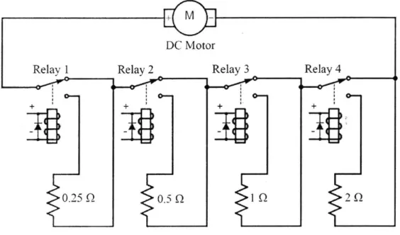
Figure 2-4: By using relays and power resistors, resistor is made.

a digitally controlled discrete variable

across the leads of the motor:

V = Ktw

When the motor is attached to a resistor R, then Ohm's law must be satisfied:

V = iR

Equations (2.1), (2.2), and (2.3) can be combined into:

T Kt2

R

(2.2)

(2.3)

(2.4)

This is the equation of a rotary damper with damping coefficient

K/R.

mod-ulating the resistance, the damping coefficient can be varied. A resistor array was built that allows for the effective resistance connected to the motor to be discretely set as shown in Figure 2-4. This system creates a viscous rotary damper that is safe, repeatable, and quiet.

The benchtop system is controlled by an Arduino microcontroller that can be Relay 3

0-D

Relay 4

2 Q

connected to a PC or Raspberry Pi. Commands are sent from the PC (or Raspberry Pi) to the Arduino via the USB serial connection. This allows for the motor speed and resistor array resistance to be set from the PC. The microcontroller also records the shaft speed via an encoder. This also allows the benchtop system to be speed controlled via a closed loop PI controller. This data is sent to the PC via the USB serial connection. A custom Python script was used to control the system from the PC which allowed for the speed and resistance settings to be automatically changed-at given intervals for easy dchanged-ata collection. Both these pieces of code can be found in Appendix C.

Most of the benchtop model was made by laser cutting acrylic panels and bolt-ing those pieces together. This includes the two base panels, the two vertical motor holding pieces, and the entire cage. This method allows for rapid and precise man-ufacturing. Furthermore, acrylic is clear and allows for viewing of the sensor during testing.

Several steps were taken to ensure that the benchtop system would be safe to operate. First, a large emergency stop switch is in line with the main power, allowing a user to rapidly de-energize the system. Second, an acrylic cage was built around the exposed shaft. This cage is strong enough to stop any sensor components that may come loQse during rotation. It also prevents the user from getting hair, clothing,

or

jewelry

cage is closed. If opened, the controller stops the motor.

To be a valid testing system, the benchtop system must have anomalies for the sensor to detect that are analogous to issues on the TEX. For example, the auger of the TEX can break, incorrect material can be used, or an operator can make an error. The chosen method was to add an off-center weight to the shaft, causing an imbal-ance. This leads to vibration in the shaft. This bending and vibration phenomena is far simpler than the coupled bending of the TEX shafts. However, this weight is enough to model a basic bending mode of the TEX. The project sponsor deemed this "issue" as sufficient for developing the anomaly detection algorithms. Non-complete engineering drawings of the benchtop system are in Appendix A. Wiring diagrams

Chapter 3

Torque and Bending Sensor

3.1

Background

Torque sensors are used for many functions. As mechanical power through a shaft is equal to angular speed times torque, they can be used in conjunction with a speed sensor to measure power usage or output. They are also often used for testing, especially when checking maximum strength or fatigue characteristics of parts or systems. They can be used in closed-loop feedback control as well as safety and health monitoring.

While there are many torque sensors already on the market, almost all are unsuit-able for this application. An example is shown in Figure 3-1. Most do not work for rotating shafts. Of those that do, most are in line with the shaft. Of the remaining ones, most are too bulky, too expensive, and/or require modification of a shaft. This application requires a small, inexpensive, and minimally invasive sensor.

Nearly all torque sensors measure strain or displacement in order to estimate torque. The most common type of torque sensors for rotating shafts have their own axle that needs to be connected to the shaft on both ends. This means the shaft needs to be cut for the sensor to be installed, making installation a long process. If the device was not originally designed for the sensor, it may not be possible to install this type of torque sensor. For example, the shaft may not have a long enough exposed portion for the sensor to be added with couplers.

Figure 3-1: An example of a production torque sensor. Image from [35].

Clamp-on sensors solve this problem by allowing installation without modifying the shaft. These devices can use several different methods to determine strain. Sur-face acoustic wave (SAW) methods induce and measure waves that are affected by strain, allowing torque to be determined [16]. These require careful mounting of com-ponents on the surface of the shaft. Other optical devices measure the deflection of precise disks spread out axially over the shaft [42]. However, the simplest way is to mount strain gauges directly onto the shaft. Unfortunately, like the SAW methods, this requires precision and many steps in the installation process [32]. In addition, the shaft is often narrowed in the section where measurements are taken, further complicating the process and weakening the shaft.

One way to ease the installation process is to create a device that deforms with the shaft and measure the strain on that device [17][201. This allows most of the calibration and precise work to be done prior to installation. Furthermore, strain gauges can be used to read the torque without direct mounting. In addition, these devices can be very compact compared to many standard torque transducers.

Strain Gauge

Bridge

Collars

Figure 3-2: A simplified diagram of the designed torque sensor.

3.2

Design

Strain induced by torque or bending of the shaft is transferred to part of the sensor,

where it is transduced into a signal. As shown in Figure 3-2, two aluminum collars

are attached tightly to the shaft so there is a given distance between them, d,. As

the shaft is torqued, one collar will rotate slightly relative to the other one. As the

shaft is bent, one side of the collars will move closer to each other while the opposite

sides separate. A plastic bridge (or multiple bridges) are used to connect the collars.

As the collars are thick and aluminum, they are far more rigid than the thin plastic

pieces. This means that nearly all displacement and therefore strain is transferred to

the bridge. Furthermore, the bridge is designed to transfer all strain to the flexure

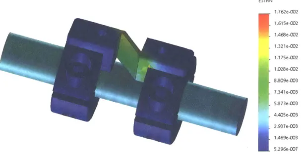
zone. This is confirmed with finite element analysis as shown in Figure 3-3. More

details of this analysis are shown in Appendix F. A strain gauge (or gauges) is placed

on the flexure zone, allowing for strain to be transduced. In addition, the plastic

bridges are far less stiff than the shaft, so the sensor does not contribute significant

stiffness to the shaft.

ESTRN 1.762e-002 S1. 615 e-002 1,468e-002 1.321e-002 1.175e-002 1.028e-002 8.809e-003 7.341e-003 5.873e-003 4.405e-003 2.937e-003 1.469e-003 5.296e-007

Figure 3-3: Finite element analysis on the sensor confirms nearly all strain occurs in

the flexure zone of the bridge.

One advantage of this sensor over other ones is that it allows the strain induced

by torque to be measured in tension instead of in shear. This allows for the use of

less expensive and more common strain gauges.

3.2.1

Torque Calculations

With the assumptions, it can be shown that the strain experienced by the sensor

is linear with the torque in the shaft. For a shaft of length Lshaft, polar moment of

inertia J, and shear modulus G undergoing torque T, the angular displacement about

the axial direction,

is

[40]:

00

GJ

If the collars are mounted such that the separation between them is d, as shown

in Figures 3-4 and 3-5, then the angle of deflection between them is simply:

Td~

G0

=

J

(3.2)

G J

Lflexure,z

is the initial length of the flexure in the axial direction as shown in Figure

x

de

}

L flexure,z

Figure 3-4: Definitions of variables used when sensor is not undergoing torque.

}

x

Figure 3-5: Definitions of variables used when sensor is undergoing torque. de

'I

direction as shown in Figures 3-4 and 3-5. The relative deformation in the angular direction, 6, at a distance r from the axis is simply:

6(x) = L 9or (3.3)

Lflexure,z

Evaluating this at x = Lflexure,z to show the total change over the bridge, 60, is:

6

O = Oor (3.4)

The plane of the flexure is 45 deg offset from the axis of the shaft. The flexure's initial length in the axial direction, Lflexure,z, remains approximately constant. The flexure's length in the angular direction, Lflexure,6, changes by 6. Geometrically, Lflexure,O and

Lfexure,z are equal and the overall initial flexure length, Lflexure,O is simply:

LflexureO = j(Liexureo)2 (Lflexurez)2 = vF2Lflexure,z (3.5)

The strain along the flexure, flexure, is simply the change in length over the original length. Using Equation (3.5), the strain is:

6f lexure - V1(LflexureO + 6o)2 + (Lflexure,z )2 - \/2Lflexure,z (3.6) \/=Lf(exurez

Combining Equations (3.2), (3.4), and (3.6) and noting that Lflexure,o and Lflexure,z are equal:

Ef lexure -

y

vL = (.exurez

Now, fEflexure is a function of T and some geometric parameters. The following Taylor approximation can be made:

Eflexure(T) 6f lexure (To + AT) 6f lexure (TO) + dEflexure AT (3.8)

Using, To = 0 it is clear that Eflexure(To = 0) is simply 0. In this case, AT = T. Now Equation (3.8) simplifies to:

Eflexure(T) e dfiexure T

dT T=O

Taking the derivative:

df Iexure

dT

1 2(Lflexure,z + r)

V Lflexure,z 2 (Liiexurez

+

+

(3.10)

Evaluating Equation (3.10) for T = 0:

(3.9)

dEflexure 1 2(Lflexurez) rdr

dT

rd,

2GJLfLexur-e,z (3.11)

Combining Equations (3.9) and (3.11) yields:

Eflexure(T) = rd T

2GJLflexure-z (3.12)

For a shaft with a circular cross-section, the polar moment of inertia, J, is simply a function of the shaft diameter., D:

rD4

32 (3.13)

Combining Equations (3.12) and (3.13) yields the final equation for strain on the flexure:

(3.14)

Eflexure(T)

16rd

'7GD4Lf lexure,z

It should be noted that it if the gauge is mounted on the surface, then r = D/2 and

dc = Ljlexure,z. In this case, Equation (3.14) reduces to:

8

'Efexure(T) ~ 8 T

irGD3 (3.15)

3.2.2

Bending

Unlike most torque sensors, this sensor is also designed to detect bending of the shaft in certain conditions. This bending is in the same signal as the torque, as a bend causes the flexure to extend or compress. While in some cases this may be considered a disadvantage as bending can disrupt the signal, it is an advantage in others. There are two forms of bending on a shaft. The first is a force applied in a direction fixed to the stationary reference frame (the observer's point of view), which would appear to rotate in the rotating reference frame (the shaft's point of view). The second is the opposite, a force that appears stationary in the rotating reference frame but rotates in the stationary one. This sensor will detect the first as a fluctuation in torque: it will cause a positive error in one orientation and a negative in the opposite. The second will be a constant error in the torque reading. Calibration at zero torque can remove the effects of the second.

If the torque is relatively constant within a rotation, bending and torque can be easily extracted from the signal. The signal can simply be averaged over a rotation to find an accurate torque. Furthermore, the fluctuation of the signal in a cycle of the shaft can be used to find the bending. This allows the use of one sensor to detect both torque and bending of the shaft, which is useful in cost sensitive or volume constrained applications.

Unfortunately, the bending of the shaft is far more complex than the torque and depends greatly on the design of the machine. While torque can be measured by simply knowing the shaft diameter and material, for bending analysis the location and type of supports and loads on the shaft must also be known. However, if these are known, the calculations are quite simple.

3.2.3

Instrumentation

The change in resistance of the strain gauges is slight, so careful instrumentation is critical to measure an accurate torque. It is standard practice to use a Wheatstone bridge to turn the change in resistance to a measurable voltage chain. As shown in

Q u

re

Br____ic-

-...

..he

..

.

Quarter

Bridge

v

RV r

Half Bridge

Full Bridge

V

Figure 3-6: Strain gauges can be used in the quarter, half, or full bridge configurations. Arrows facing apart represent a gauge undergoing tension while arrows facing each other represent a gauge undergoing compression. Image modified from [4].

Figure 3-6, the Wheatstone bridge can be used in the quarter, half, or full configu-ration. Changes in temperature can change the resistance of the gauge, and, in the quarter bridge, this can cause significant error. However, in the half bridge and full bridge configurations, these changes are largely canceled out if all the gauges expe-rience the same thermal effects. Furthermore, the signal strength of the half bridge is double that of the quarter as the half bridge is simply two quarter bridges super-imposed. For the same reasons, the full bridge has double the signal strength of the half bridge and four times that of the quarter bridge.

A change in resistance of a strain gauge AR is related to the static resistance of the strain gauge R, the gauge factor GF, and the strain it experiences, Egauge by the following equation [33]:

_ AR

Rcgauge

Using simple voltage divider equations, if V, is applied to the top of a bridge and the bottom is grounded, then the voltage across the bridge V is simply:

~(

R4

R2+R4

(3.17)

are stretched and R2 and R3 are compressed. Using AR from Equation (3.14) and

the fact that all resistances when unstretched are R, the voltage across the bridge will be:

(

(R+ AR)

(R)

(.)

(R - AR) + (R + 2KR)

(

_R + AR) + (R - AK)

This equation can be simplified to:

V = V A(3.19)

R

Combining Equations (3.16) and (3.19) yields:

Egauge - = V

(3.20)

As the gauge is glued to the flexure, it can be assumed that their strains are approx-imately equal. Using this approximation and Equations (3.14) and (3.20):

T= VLjiexurez GD (3.21)

16 V, d, GFr

Most common strain gauges can only handle up to about 2% strain and have a gauge factor of approximately 2 [331. Many microcontrollers operate at 3.3V or 5V

[7].

Now that the maximum voltage is known, a chip to amplify and digitally read the strain gauges can be specified. It should be able to measure a voltage of 0.20 V before any safety factor. Furthermore, the lowest possible noise, highest possible resolution, accuracy, and highest sample rate are ideal. Two possible chips are compared in Table

3.2.3. While the LTC2440 has better specifications, it is much harder to integrate

into the system. To utilize it, a custom printed circuit board (PCB) would have to be fabricated. Therefore it is much easier to use the HX711 which has already made breakout boards. However, some non-rotating results have been collected with the

HX711

LTC2440

Resolution (bits)

24

24

Max Sample Rate (Hz)

80

3500

Voltage Range (V)

0.5

2.5

Table 3.1: Comparison of two chips that can be used

is from [10] and LTC2440 data is from

1211.

to read the strain. HX711 data

Figure 3-7: A rendering of the novel torque sensor.

LTC2240.

3.2.4

Construction

The sensor is relatively simple to produce. Furthermore, many of the parts can

be made with relatively low precision without significantly affecting the accuracy of

readings. Many of the tolerance issues can be corrected by calibration after the sensor

is assembled. Engineering drawings of the prototype are presented in Appendix A

and wiring diagrams are shown in Appendix B.

Figure 3-8: The new torque sensor as made.

Modified Collars

CollIar

Bridge

ain G

Bridge

V

Bolts

Figure 3-9: Exactly half the parts required for the torque sensor.

00i

Figure 3-10: The aluminum collars before (left) and after machining (right)

The first step is to machine standard shaft collars into the collars used in the sensor. First, a facing cut is used to add a flat face on the cylindrical surface. Next, a hole is drilled and tapped in the flat face. This operation can be completed with fixing the part once in a manual mill. The initial and final collars are pictured in Figure 3-10.

Next, the bridge must be fabricated. The version in the prototype was 3D printed with acrylonitrile butadiene styrene (ABS) using the fused deposition method (FDM). The flexure zone thickness was limited by the resolution of the printer used (a Strata-sys Fortus 250mc).

Final assembly is quite easy. Strain gauges are glued to the flexure zone of the bridge. Strain gauges should then be soldered to the ADC chip. The bridges are then bolted to the collars. The collars are then bolted to the shaft. It is helpful if the sensor is read while the collars are being bolted to ensure the sensor is not saturated

by a misalignment. More details of this process are presented in Appendix G.

Oii'm _{" A}

3.3

Results

3.3.1

Stationary vs. Rotating Shafts

Rotating the device requires significant development of other components of the sen-sor. First of all, wireless communications or power must be installed. In addition, all components must be secured to withstand the considerable centripetal forces experi-enced while spinning. Finally, it is difficult to induce known dynamic torques. While a known static torque can be easily applied by measuring a force on a lever, no such simple solution exists for spinning shafts.

Rotation can also add several phenomena that can interfere with calibration of the sensor. First, if the shaft is relatively thin, the weight of the sensor can cause bending (this is useful in Section 3.3.3) which interferes with the calibration. Vibrations caused by a number of sources, such as ball bearings or slight shaft imbalances, also cause noise in the torque signal.

3.3.2

Stationary Results

For these reasons, the sensor was initially tested while stationary. One end of the shaft was fixed while a torque was applied to the other end. All tests in this section were done with a 3/8" (9.5 mm) aluminum shaft.

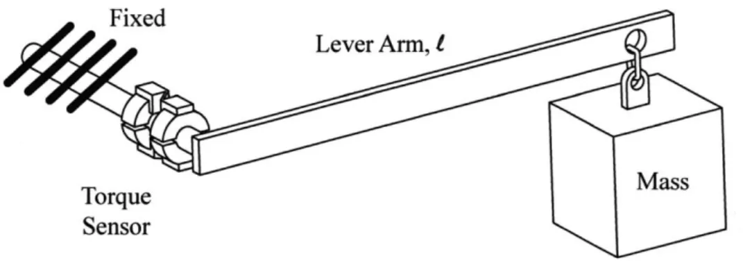
In the first experiment, different weights were applied to a lever arm to induce a known torque on the shaft as shown in Figure 3-11. The lever arm used was 142.5 mm in length and the weights varied from 2.4 N to 12.7 N. This results in torques from 0.34 N m to 1.81 N m. The output from the torque sensor, Ts, and the calculated applied torque over time are shown in Figure 3-12 and Figure 3-13. As shown in Figure 3-14, these results are very linear. Furthermore, the scaling factor is consistent while the zero offset does drift some.

This experiment shows several important characteristics of the sensor. As shown in Figure 3-14, these results are very linear. In the figure, 750 to 1000 points were averaged for each experimental data point. As the mass was manually changed,

Fixed

Lever Ann, 1

Torque

Mass

Sensor

Figure 3-11: The experimental setup used to calibrate the torque sensor by varying

the weight applied on the lever arm (not to scale).

the quickness of the sensor response cannot be accurately calculated from this data.

However, it is clearly less than one second. Some of the noise at steady state can

be attributed to the nature of the setup: the force exerted on the lever arm by the

weight is subject to airflows on the weight in the room where it was tested. Finally,

some of the offset drift can be seen at the first torque reading and the first two zero

readings in Figure 3-12. This is part of the warm-up of the sensor.

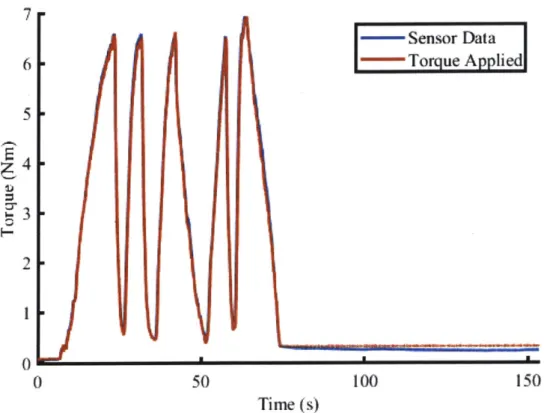
In the second experiment shown in Figure 3-15, a force meter was used to measure

a varying force, F, applied on a lever arm of f. The results of this experiment are

shown in Figure 3-16. It is clear that the sensor tracks the changing torque fairly

accurately. The drift can be seen towards the end of the sample. In addition, small

errors can be seen at high torques, indicating possible saturation.

3.3.3

Rotating and Bending Results

In order to collect data from a rotating the shaft, the sensor and shaft were inserted

into the benchtop system described in Section 2 and shown in Figure 2-2. As the

shaft is supported on both ends, the weight of the sensor causes the shaft to bend

downwards. When the shaft rotates, the bending force rotates from the shaft and

sensor's perspective. This creates a fluctuating bending. Therefore, at a constant

angular speed and torque, the signal should be a sine wave. The frequency is the

angular speed of the shaft, the amplitude is the amount of bending, and the offset

is the torque. As the bending remains stationary while the shaft rotates, this should

Calibrated Sensor Data over Time

Meaured

500

1000

1500

Time (s)

2000

2500

Figure 3-12: Output of the torque sensor and applied torque over

Calibrated Sensor Data over

Time

- M ea

ured

-- Actual

350

400

450

500

550

600

650

Time (s)

Figure 3-13: A zoomed in view of Figure 3-12.

1.5

I-0.5

-

01--0.5

0

3000

time.

1.5

0.-~0.5.

0

700

-0

M

M

2

Time Averaged Data

1.5

0.5

,0'

Expiremental Data

0

0.5

1

1.5

2

Torque (Nm)

Figure 3-14: The output of the torque sensor versus the applied torque. The

rela-tionship is linear. The raw data is presented in Figure 3-12.

Lever Armn, I

Fixed

Figure 3-15: The experimental setup used to calibrate the torque sensor using a

purchased force meter to measure applied on the lever arm (not to scale).

7r

5

2

1'

0'

I-Sensor

Data

Torque Appliedi

50

100

150

Time (s)

Figure 3-16: Output of the torque sensor and applied torque over time.

cause the signal to fluctuate between the positive and negative amount of strain

induced by bending plus the strain caused by torque.

Due to the reasons explained in Section 6.2, the sensor samples in bursts rather

than continuously. One of these bursts is pictured in Figure 3-17. As expected, it

appears to be a sine wave. As apparent in the figure, there are cyclical anomalies

every other cycle. The cause of this is unknown. However, the power spectrum of

this signal, shown in Figure 3-18, indicates that occurs at around 4 Hz.

In a separate but similar experiment, the sensor was run at various speeds and

the power spectrum was taken of the signal at each speed. As shown in Figure 3-19,

the dominant frequency is at the shaft speed.

3.3.4

Long Term Drift

The most significant issue is the drift in the reading over long periods of time. This

occurs with both the HX711 and LTC2440 chips as shown in Figures 3-20 and 3-21,

0 0

0.2

Figure 3-17: A burst reading from

reading and the amount of bending

the angular speed of the shaft (600

0.8

0.6

S0.4

0.21

the torque sensor

as the amplitude.

RPM or 10 Hz).

shows the torque as the mean

The frequency of the signal is

0

0 5 10 15 20 25

Frequency (Hz)

Figure 3-18: The power spectrum of the signal show

dominant frequency of 10 Hz.

30 35 40 45

n in Figure 3-17 shows the clear

I

0

I

Vj

1

1000

500

0

1000

500

0

2.3 Hz

1000

500

0

0

0 Hz

0

10

20

R

F (Hz)

4.5 Hz

0

10

20

3C

F ( Hz)

10.6 Hz

10

20

30

0

F (Hz)

I

10

20

30

F (Hz)

7.6 Hz

0

10

20

3

F (Hz)

14.4 Hz

10

20

30

F (Hz)

Figure 3-19: A power spectrum of the torque signal shows that the dominant

fre-quency of the signal is the shaft speed (title of each graph).

1000

500

0

1000

500

0

1000

500

0

)

0

500

71-0

-500

0

10

20

30

Time (hr)

40

50

HX711 Drift

50.0.

Figure 3-20: Drift in the sensor reading over time with the HX711 chip.

respectively. In these experiments, the sensor was stationary with no applied torque

on the shaft. This is common with strain gauges and is often attributed to various

thermal effects [18].

Therefore, it may be possible to measure temperature and use it to correct the

strain reading. As shown in Figure 3-20, measured strain with the HX711 and

tem-perature appear to sometimes be correlated and other times not. For the first 20-25

hours, they seem to be correlated. The large spike in measured strain at the end

can be attributed to the battery dying. Similar results are found with the already

lower-drift LTC2440, shown in Figure 3-23. There appears to be a correlation

be-tween strain and temperature after about 27 hours, but not before. The temperature

versus measured strain is shown for each chip in Figures 3-22 and 3-23.

Using a linear fit, a correction can be applied. For example, if only the data from

times between 25 hours and 32 hours are taken from Figure 3-21, then the correlation

is very strong as seen in Figure 3-24. The linear fit can then be used to correct the

6-21.4

21.6

13.2

40

30

20

10

-0

-10

-20

LTC2440 Drift

10

20

30

40

Time (hr)

50

60

22.8

22.6

y

2.IA

"

"

Figure 3-21: Drift in the sensor reading over time with the LTC2440 chip.

1-.1

HX711 Temperature vs. Strain

21.6 21.8 22 22.2 22.4 22.6 22.8 23 23.2 Temperature (C)

Figure 3-22: Chip temperature versus strain reading for the HX711 chip. The corre-lation appears to be weak.

.- I-" Ii"

Li>

.

.

.

.N

1

221

70

0

M

"M

.

30

22.2 22.3 22.4 22.5 22.6 22.7

Temperature (C)

22.8 22.9 23

Figure 3-23: Chip temperature versus strain reading for the LTC2440 chip. There

appears to be some very weak correlation.

signal. If xt is the temperature reading and yzero is the strain reading at zero torque,

regression can be used to find linear constants a, and b,:

Yzero ~ ar * xt + br

(3.22)

Using this analysis, the corrected strain, Ycorrected, from the strain input Yraw and

temperature input xt is approximately:

Ycorrected - Yraw - ar * xt - br

(3.23)

This correction is shown in Figure 3-25. While this methodology was not

imple-mented into the sensor, it could easily be done before any production.

Even without corrections and with the LTC2440 chip, the sensor has reasonable

stability over a given minute or hour. As shown in Figures 3-26 and 3-27, the drift

in the short term is quite minimal. This means that the sensor can retain reasonable

accuracy as described in the figures if calibrated every hour (or minute). It should

49

0i~~~'111lii

ii

ll I

-ii

i-NI~iIIII

.10

-22

---

--

-5

0 10

22.4 22.45 22.5 22.55 22.6 22.65 22.7 22.75 22.8 22.85 Temperature (C)

Figure 3-24: Chip temperature versus strain reading for the LTC2440 chip for times

25 hours to 32 hours as shown in Figure 3-21. The correlation is strong and a linear fit is shown. 8 6 4 r -Original Data - Corrected Data 25 26 27 28 29 Time (hr) 30 31 32

Figure 3-25: Temperature correction

of the LTC2440.

factors can be applied to improve the reading

Dat * -Fit I-U) I-U)

-5

-2

Range of Strain over I Minute 0.2 0.15 1

0.1

1

Figure 3-26: The probability distribution of total strain drift

majority of samples have less than 2 micro-strain of drift.

over a minute. The vast

be noted that the samples used here were truncated from earlier figures. The drift at the very beginning of some of the earlier samples is attributed to "warm-up" and some at the end is due to the battery voltage dropping. In most cases, the warm-up was found to be around 20 to 30 minutes.

I I I A "1 L-2 2 22.4 . . . .

Range of Strain over I flour

u . . .

-1

3 4 5 6 7 8 9 10 Micro-Strain

Figure 3-27: The probability distribution of total strain drift over is on the order of micro-strains.

an hour. The drift

0.3 0.251 0.2 r 0.15 I-0.1 0.05 I 0 w-.4

Chapter 4

Acceleration

Measuring the speed and vibration of the shaft is critical for the sensor. Speed is the flow variable of the shaft system and can be used to determine power. It is also one of the critical parameters of the TEX. In addition, vibrations are common symptoms of problems in machinery. By utilizing an accelerometer and associated methods as described in this section, both speed and vibrations can be measured.

4.1

Theory

As with torque, many solutions exist for measuring shaft speed. Hall effect sensors can be used to determine when a point on the shaft passes by. Differentiating this signal produces the angular speed [311. Similarly, encoders and photo tachometers track when parts of the shaft pass and differentiate for speed [15]. In addition, motors can be driven by the shaft and the output voltage is approximately proportional to the speed [13J.

However, most of these methods require fixed components that do not rotate with the shaft. An accelerometer, however, can rotate with the shaft and is relatively inexpensive. There are at least three ways to estimate rotational speed from an accelerometer attached to the shaft: angular integration, centripetal acceleration, and frequency analysis. Furthermore, an accelerometer can be used to detect the frequency and amplitude of vibrations present on the shaft [34]. This frequency data

can be useful in detecting problems in the system.

Integration of the angular acceleration causes significant error. This is similar to how accelerometers are used to estimate position and has the same issues. If there is any calibration error, then speed will be read as constantly increasing or decreasing even if the angular speed is constant. Therefore, this method is not used.

Determining angular speed precisely from the magnitude of radial acceleration requires accurate calibration. If the radius of the shaft r., is known and the magnitude of the centripetal acceleration (radial direction) is ac, then the angular speed w is

as given by Equation 4.1. The downside of this approach is that it requires the accelerometer to be calibrated accurately, although it is not as sensitive to calibration as the integration method. Any error in a, directly affects the estimate of w as shown in Equation (4.1).

W = r (4.1)

Gravitational effects affect the readings of radial and angular acceleration in most non-vertical and rotating shafts. While this effect may be insignificant relative to the centripetal acceleration, it can also simply be averaged out if the sample rate is high enough. If enough data points from the signal are averaged through a cycle or across cycles, the gravitational effects in each individual data point cancel. In fact, these effects complement each other: at high speeds the centripetal acceleration is high so it minimizes the gravitational effect in the signal while at low speeds it is easier to have faster sampling relative to the shaft speed.

Analyzing the frequency of the radial or angular acceleration signals is this most resilient of the methods in some conditions. If the shaft is not vertical, at the radial and angular signals will fluctuate within a rotation due to gravity. In the case of a horizontal shaft at constant angular speed, one would expect the angular acceleration to vary from positive g to negative g each rotation, where g is the acceleration of gravity. When the accelerometer is on the top of the shaft, it will read zero angular acceleration. A quarter-turn later when it is on the side, it will read plus or minus

3500

No Noise Speeds

3000

2500

-

Speed

_Centripetal

2)000

_-

_Integrated

5

FFT(Y)

1500

500

0

0

5

10

15

20

Time (s)

Figure 4-1: A simulation of the calculated speed from the accelerometer using three

different methods assuming no noise in the signal.

g, depending on the orientation. Another quarter-turn so it is on the bottom of the

shaft will make it read zero once again. Finally, one more quarter turn will put it

on the opposite with a reading of minus or plus g. Similarly, the radial acceleration

would vary from a, + g to ac

-

g. As long as the sampling rate is sufficiently high (at

least twice the angular frequency) and the angular speed does not change rapidly, a

power spectrum will clearly show the angular speed as the dominant frequency in the

signal.

In the simulation shown in Figures 4-1, 4-2, and 4-3, a shaft starts at rest and

is constantly accelerated to 1000 RPM (16.7 Hz) over 10 seconds. It then spins at a

constant speed for 10 more seconds. The accelerometer is simulated as being 12.5 mm

from the axis of rotation. The code used to run this simulation is included in Appendix

D. All the signals oscillate as the accelerometer is rotating relative to gravity. It is

clear that even with perfect signals as shown in Figure 4-1, the integration method has

a substantial error. This is due to the effects of gravity. Whenever the accelerometer