HAL Id: hal-02486791
https://hal.archives-ouvertes.fr/hal-02486791
Preprint submitted on 21 Feb 2020
HAL is a multi-disciplinary open access
archive for the deposit and dissemination of sci-entific research documents, whether they are pub-lished or not. The documents may come from teaching and research institutions in France or
L’archive ouverte pluridisciplinaire HAL, est destinée au dépôt et à la diffusion de documents scientifiques de niveau recherche, publiés ou non, émanant des établissements d’enseignement et de recherche français ou étrangers, des laboratoires
Employment, unemployment, participation and
migration: a regional study
Pierre Lesuisse
To cite this version:
Pierre Lesuisse. Employment, unemployment, participation and migration: a regional study. 2020. �hal-02486791�
Employment, unemployment, participation and migration:
a regional study
LESUISSE Pierre
CERDI - University of Clermont Auvergne, [email protected]
février, 2020
Résumé
Despite GDP growth rate higher than EU-15 average, labour market conditions in some Central and Eastern European countries remain under question. Indeed, the unemployment rate takes time to decrease closed to or below the European average and the participation rate remains under European standards. This non-employment is even more an issue when looking at the regional NUTS-2 level where the dispersion increased over time. We use theBlanchard et al.(1992) approach to understand the reactions of both unemployment and participation rates when a shock is imposed on employment, at the regional level. We focus on the CEECs, using a panel-VAR estimation and draw an overall comparison with EU-15 countries. We identify two adjustment channel through wages and unemployment. We find an efficient labour supply adjustment in both group. The response of the unemployment rate is slightly more persistent and the women participation is more vulnerable in the CEECs. Keywords : Labour market, Unemployment and participation rates, European Union, panel VAR.
1
Introduction
The Europe 2020 growth strategy aims at a greater coordination of national policy in the European Union. Set for a ten-years period in 2010, one of the five main pillars states a six percentage points (pp) increase in the employment rate of the 20-64 years-old population (from 69% to 75%). During the 2010-2018 period, the employment rate in-creased on average in EU-28, to 73.1%. The boost was particularly impressive in Central and Eastern European Countries (henceworth CEECs), where it increases from 65.5% to 74.3%. In comparison, it grew by less than 3.5 percentage points (pp) in the EU-15 group. While employment level expands, by five percent in both group of countries, the denominator of the employment rate, the working age population, remained stable in the EU-15 group and decreased by six percent in CEECs. From this perspective, the employ-ment rate change in the CEECs seems to be relatively labour supply driven compared to the change in the EU-15 group.
It is in this specific context that we find interesting to look at the dynamical changes upon the labour markets in the CEECs and to draw a comparison with the EU-15 econo-mies. Indeed, the CEECs labour markets functioning are almost systematically pointed out in the country specific recommendations of the 2018 European Semester.
The purpose of this paper is to disentangle the labour market’s mechanisms, when an exogenous shock affects the level of employment. We replicate theBlanchard et al.(1992) approach and observe how an employment innovation is absorbed on the labour market. Focusing on the employment, unemployment and participation rates, we expect a positive innovation on the labour demand to temporarily stimulate the labour force participation rate and decrease the unemployment rate, ending up with a permanent higher level of employment.
Our contribution in this field is threefold. First we update and enrich the work of
Gacs and Huber(2005) who covered the 1992-1998 period. We are convinced that looking at the period after 2000 may give some new insights and allows us to deal with harmo-nized data at the regional level (NUTS-2). The focus on the 1999-2017 period avoids structural reforms, following the transition in the nineties, to deteriorate our estimations leading to identification issues.
Second, we implement a robust comparison between the CEECs and the EU-15 group to understand whether the different labour markets tend to converge in terms of labour market response following an exogenous shock. Similar reactions could give weight to the European employment policy efficiency.
Last, following European Commission and Directorate-General for Employment(2018), who highlight the gender gap issue on the labour market, we provide a gender distinction which support the IMF and the Europe 2020 strategy recommendations concerning the weak Women labour force participation in the CEECs.
Following a positive shock imposed on the labour market, the level of employment permanently reach a higher level ; while both participation and unemployment rates impacts fade out within a decade. Drawing a comparison between the EU-15 and the CEECs, we find a relative more persistent response of the unemployment rate in the last group. By construction, the employment innovation is absorbed through wages and unemployment adjustments. The employment level ends up at a slightly higher level in the CEECs. This reflects a more efficient unemployment channel and underlies a relative more responsive labour supply in case of employment shock.
A specific focus on the participation rate dynamics allows us to exacerbate the women vulnerability in the CEECs relative to both men in CEECs and women in EU-15. We so pointed out, the necessity to implement reforms favouring women labour force partici-pation rate for example thanks to childcare program in order to target the most at-risk population in case of employment shock.
The section 2 of this paper gives an overview of the existing literature. The section 3 describes the data and presents some stylized facts. The section 4 proposes the empirical strategy while section 5 presents the main results. Then, the rest of the paper is divided in two sections ; the section 6 discusses the results and the last section concludes.
2
Literature review
The transition process in the CEECs started in the nineties and implied a newborn unemployment induced by restructurations, privatizations and a labour to capital substi-tution (Aghion and Blanchard,1994;Blanchard,1998). Looking at transition economies in Europe and Central Asia,Rutkowski (2006) highlighted a correlation between the re-structurations and the drop in the observed employment rate. According to Bornhorst and Commander (2006) and Münich and Svejnar (2007), focusing on the first decade of the transition in the CEECs, the production factors substitution was not followed, in the short run, by a net creation of employment. At the same same, labour market
institutions, mostly through their non-employment benefits programs1, do not stimulate labour mobility, leading to regional disparities and weak wage adjustment (Boeri and Scarpetta,1996). Using a four-countries panel (Bulgaria, Czech Republic, Hungary and Ukraine) at the NUTS-3 level, in 2001,Jurajda and Terrell(2009), pointed out the weak labour mobility induced by the low efficiency of labour market institutions to explain the lack of convergence of the unemployment rates across regions.
According to Campos and Coricelli (2002) the low labour mobility across regions, signi-ficantly impacts the persistence in high unemployment rate and the weak participation rate.Fidrmuc(2004), using data on Czechia, Hungary, Poland and Slovakia, covering the 1992-1998 period confirm a regional mobility issue.
Empirical analyses, fromSvejnar(1999) andHuber(2007), looking at the regional dimen-sions, highlight an improvement of labour market conditions, only in economic centers and regions geographically closed to the EU-15 (i.e. sharing a common border with wes-tern European countries).Gacs and Huber(2005), looking at a panel of CEECs NUTS-3 regions, draw a comparison between rural and urban labour market adjustments. They analysed changes in employment and the impact on unemployment and the participation rate. They found rural regions to be left behind. Regions, away from economic center, do not take advantage neither from economic development nor from public or private investments.
According to Marelli et al. (2012) or Rios (2016), this regional heterogeneity is still present. Over a more contemporaneous period, they disentangle the labour market evo-lution before and after the 2008 economic crisis. They draw a spatial analysis in both EU-15 and CEECs groups and found a persistent heterogeneity in regional labour market response after shocks.
Nevertheless, the labour market institutions in the CEECs played a significant role, compared to Former Soviet Union economies, to foster the CEECs in their transition pro-cess (Boeri and Terrell,2002). This corroborates Huber (2004) looking at the evolution of regional labour markets in the CEECs before their accession to the European Union.
The fog on the labour market developments in CEECs may also be explained by a skill-mismatch problem implying a relative more persistent unemployment compared to Central Asian transition economies which suffered more from underemployment ( Rut-kowski,2006). The new private labour demand, does not fit the labour supply. Dealing 1. Non-employment benefits consist for example on unemployment benefits, early retirements pro-grams, welfare assistance.
with a survey of 921 firms concerning Hungary, Romania and Russia in 2000, Comman-der and Kollo (2008) look at the inadequacy between a low skilled labour supply versus a high educated labour demand. They found a correlation between the skill-mismatch persistence and both education spending and education quality to explain the persistence of the weaknesses of the labour market.
However, the observed recent fall in the unemployment rate, confirmLeón-Ledesma and McAdam(2004) who reject the hysteresis hypothesis even during the first decade of the transition.
3
Data
3.1 Data description
This study considers a regional approach at the European level (28 countries). Two main groups of countries are analysed. The first group includes the EU-15 states, i.e. the fifteenth first EU members while the second group focus on CEECs. We use the EU-15 group as a benchmark to allow comparison inside the EU-28.
We adopt the use of NUTS-2 data, commonly used to analyse the EU labour market dynamics (Decressin and Fatás,1995;Gacs and Huber,2005;Halleck Vega and Elhorst,
2014;Beyer and Smets,2015).
Data are extracted from Eurostat website2, and cover the 1999-2017 period. As we are looking for regional interactions, we may not include in our database, countries with less than three NUTS-2 regions. We do not kept Ireland, Luxembourg, Cyprus and Malta. In the EU-15 group, we drop Finland and Denmark due to missing data. Greece has been removed because of few reliable data. Bulgaria, Croatia and Slovenia are also dropped because of missing data and smaller time span. We integrate the Baltic countries (i.e. Estonia, Latvia and Lithuania) as a "single country" with three regions.
Moreover, autonomous regions from Spain, Portugal and Italy are excluded (it concerns Ceuta, Melilla, Acores, Madeira and Aoste). Last, french overseas department and terri-tories are also dropped out. Some other regions, not providing a complete information on the overall period, are kept aside. Last, when the geographical definition changed during the period, the concerned regions are also suppressed from our database. We end up, from 1999 to 2017, with 156 regions in EU-15 group and 45 in the CEECs group.
Data are collected thanks to the Labour Force Survey (LFS), at an annual fre-2. http ://ec.europa.eu/eurostat/en/data/database
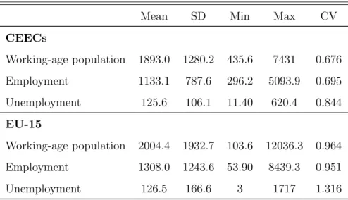
Table 1 – Regional main statistics by sub-groups
Mean SD Min Max CV
CEECs Working-age population 1893.0 1280.2 435.6 7431 0.676 Employment 1133.1 787.6 296.2 5093.9 0.695 Unemployment 125.6 106.1 11.40 620.4 0.844 EU-15 Working-age population 2004.4 1932.7 103.6 12036.3 0.964 Employment 1308.0 1243.6 53.90 8439.3 0.951 Unemployment 126.5 166.6 3 1717 1.316
Notes : The variables are expressed in thousand individuals, average by region by sub-group of countries, over the 1999-2017 period.
quency, such that the definition of the different variables are homogeneous for the whole panel. We focus on the regional working age population, employment and unemployment and consider the 15-64 yo population.3 Each variable is expressed in thousands persons. The working age population refers to every individual aged 15-64 yo at the time of the survey. Employment measure considers every person, ‘member of the active population which has, at least, worked for one hour during the period under study or which is tem-porarily absent for work’.
Unemployment is measured thanks to the International Labour Office definition, i.e. per-sons who are not currently employed but actively looking for a job. Every variables is available by sex, to allow a gender heterogeneity in our analysis.
From the beginning of the period, the working age population decreased by almost seven percent in CEECs with the highest drop in Baltic states and Romania. Slovakia is the only one country in the CEECs to end up with a positive change in the working age po-pulation (+3,4%). Employment grew by less than two percent but hides a twelve percent drop in Romania against a thirteen percent increase in Poland.
The table1presents the main statistics of the three variables by sub-group. Thanks 3. Source : Eurostat database ; last update 18/03/2019 ; extracted on 21/03/2019 ; Working age population : lfst_r_lfsd2pop ; Employment : lfst_r_lfe2emp ; Unemployment : lfst_r_lfu2gac ; it would have been interesting to also look at the 20-64 yo population nevertheless data at the regional level are not provided in this dimension.
to the use of the regional level, instead of the country approach, the variables tend to be more homogeneous in level.4 The average of each variable is at a slightly highest level in the EU-15 countries. The dispersion of the variables is smaller in the CEECs, this suggest a relatively weaker level of heterogeneity amongst CEECs regions compared to the EU-15 group. In both sub-group, the coefficient of variation (CV) of unemployment is relatively bigger than the two other CV, even larger than one, suggestion a high level of heterogeneity in unemployment data. The regional dimension seems to be even more justified when looking at the unemployment level.
3.2 Stylized facts
Before going further, we compute the employment rate, defined as the ratio of em-ployment over the working-age population ; the participation rate, defined as the sum of employment and unemployment over the working age population ; last the unemployment rate, which is the ratio of unemployment over the active population i.e. unemployment over the sum of employment and unemployment.
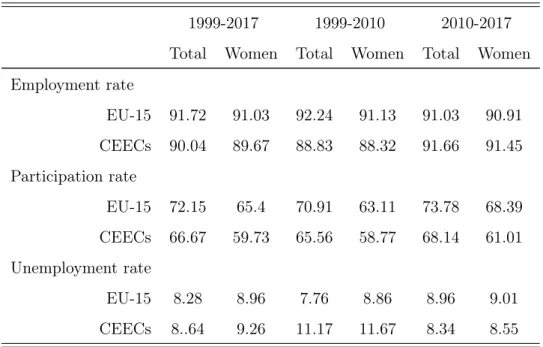
The employment rate in the CEECs is closed to but below the EU-15 level (table
2). However from 2010 to 2017, the employment rate reaches 91,66% of the working age population, 0.5pp higher than in the EU-15 group. In the CEECs, Czech Republic is the best performer with the highest employment rate (94.12%) and the lowest unemployment rate (5.88%). The unemployment rate slightly decreased at the end of the period, from 11.17% before 2010 to 8.34% . At the same time, it increases in the EU-15 sub-group (from 7.76% to 8.96%). Looking at the participation rate, we found a gap between the CEECs and the EU-15 countries. Despite an increasing trend, the participation rate in the CEECs remains below the EU-15 level.
The graph (1) illustrates the evolution of the unemployment and participation rates in the CEECs compared to EU-15 average. If a region5lies over the solid line in the case of participation or at the left side concerning the unemployment rate, then we may consider the country as a better performer than EU-15.6 We observe kind of a ‘convergence’ in the unemployment rate as almost every country comes closed or just below the EU-15
4. In the appendix, the tables6&7describe the variables per country. On average, EU-15 countries
are almost three times bigger than CEECs in terms of working age population. 5. Each point refers to a NUTS-2 region in CEECs
Figure 1 – Participation rate versus unemployment rate CZ01 CZ02 CZ03 CZ04 CZ05 CZ06CZ07 CZ08 EE00 HU21 HU22 HU23 HU31 HU32 HU33 LV00 PL21 PL22 PL41 PL42 PL43 PL51 PL52 PL61 PL62 PL63 PL71 PL72 PL81 PL82 PL84 RO11RO12 RO21 RO22 RO31 RO32 RO41 RO42 SK01 SK02 SK03 SK04 .55 .6 .65 .7 .75 Pa rti ci pa tio n ra te .05 .1 .15 .2 .25 Unemployment rate 2000-2009 CZ01 CZ02 CZ03 CZ04 CZ05 CZ06 CZ07 CZ08 EE00 HU10 HU21 HU22 HU23 HU31 HU32 HU33 LT00 LV00 PL21 PL22 PL41 PL42 PL43 PL51 PL52 PL61 PL62 PL63 PL71 PL72 PL81 PL82 PL84 RO11 RO12 RO21 RO22 RO31 RO32 RO41 RO42 SK01 SK02 SK03 SK04 .6 .65 .7 .75 .8 Pa rti ci pa tio n ra te 0 .05 .1 .15 .2 Unemployment rate 2010-2017 Participation vs unemployment
Source : Own calculation given Eurostat database
Each point refers to a particular NUTS-2 region of the CEECs. The two axis represent the
unemployment and participation rates computed respectively as the ratio of unemployment to labour force and labour force to working age population. The solid lines represents the EU-15 average over the same periods and allow to understand how a region stands compared to the EU-15.
Table 2 – Main statistics by group of countries
1999-2017 1999-2010 2010-2017
Total Women Total Women Total Women
Employment rate EU-15 91.72 91.03 92.24 91.13 91.03 90.91 CEECs 90.04 89.67 88.83 88.32 91.66 91.45 Participation rate EU-15 72.15 65.4 70.91 63.11 73.78 68.39 CEECs 66.67 59.73 65.56 58.77 68.14 61.01 Unemployment rate EU-15 8.28 8.96 7.76 8.86 8.96 9.01 CEECs 8..64 9.26 11.17 11.67 8.34 8.55
Notes : The variables are expressed in percentage.
average in the period 2010-2016 compared to the situation before 2010. Unfortunately, the changes in the participation rates are less conclusive. On the overall, CEECs remain below the solid line. These facts corroborates recent IMF and European Commission and Directorate-General for Employment(2018) recommendations concerning the labour market changes that has to be implemented during the next years.
As highlighted inEuropean Commission and Directorate-General for Employment(2018), and observed in table2 the positive changes in labour market variables, in the CEECs, hide a hard to fill gender gap. The women participation to the labour market remains a current issue. Despite an increasing employment rate among women and a decreasing unemployment rate, the gender gap in participation has been increasing up to almost 7.5pp, to a higher level than in EU-15, comparing period before and after 2010.
4
Empirical strategy
Blanchard et al. (1992) used a regional dimension to disentangle the interactions upon the US labour market. They formalized the US labour demand and supply and then confront their reactions in case of an employment shock. This seminal paper was
reproduced byDecressin and Fatás(1995) looking at differences between the US and EU labour markets. More recently, two new contributions enriched the paper. Halleck Vega and Elhorst (2014) introduced spatial spillovers looking at the labour market dynamics in eight Western European countries from 2000 to 2011. Beyer and Smets (2015) used multi-level factor model, on the US labour market, to extract the regional dimension in the data.
The main advantage of theBlanchard et al.(1992) approach is to give an overview of the different behaviours on the labour market from both demand and supply sides. Moreover it allows to visualize the share of an employment shock, absorbed, in the long run, by the wages or by the unemployment. Eventually, the simulation of an exogenous employment innovation easily illustrates the employment level reaction and both participation and unemployment rates changes.
To capture the dynamic upon the labour market and to deal with the endogeneity amongst the variables of employment, unemployment and participation, we use a panel VAR. The model is written as :
Yit= A1Yit−1+ ... + ApYit−p+ ui+ µct+ νct+ εit, i = 1, ..., N and t = 1, ..., T (4.1)
where Yit= (y11t, ..., yKit) is a (K ∗ 1) vector of endogenous variables. The Aj correspond
to the coefficients matrices, and are on (K ∗ K) dimension . The vector ui = (u1i, ..., uKi ) is a (K ∗ 1) vector of individual fixed effects and εt= (ε1it, ..., εitK) is an i.i.d. residuals
vectors with zero mean and fixed variance (E(εit= 0) ; E(εitε0it= Ω.It = s) ∀i and t).
The temporal and individual dimensions are respectively introduced through the t and i indices.
As we are implementing a panel approach at the European level, we have to deal with two different levels. The first one considers the different countries, member of the European union then the second level consists of the regional breakdown of these countries. The regional dimension will be considered thanks to the regional fixed effect introduced in our specification. Unfortunately, the country dimension may not be taken into account. To deal with this issue, we built a proxy of the country fixed effect using employment in all regions of the country, except the region under study. As we use all the other regions of a specific country and not only neighbouring regions, we do not count for regional spillovers but the common evolution in a specific country.7
7. As for an example, we think that employment in Karlsruhe (south Germany) may not im-pact employment in Hamburg (North Germany), otherwise than by the German overall macroeconomic policies.
The higher the number of regions, the more efficient the proxy will be. This point confirm the use of NUTS-2 data to the detriment of NUTS-1, less reliable in the context of our analysis. Obviously, countries with less than three NUTS-2 region are excluded from our panel (exception concerning the three Baltic countries treated as a single country as pre-viously mentioned) :
µct= employmentct− employmentit with employmentct = I
X
i=1
employmentit
where i the regional dimension, c the country level, t the temporal dimension and I the total number of regions inside the country c. We also add a country specific time trend (νct) such that νct= µc∗ trend.
In panel specification, when the individual dimension (N=45 in the CEECS and N=156 in the EU-15 group) is overwhelming a fixed temporal horizon (here T=19), the least square dummy variables estimator (LSDV) leads to inconsistent estimation of the parameters of interest. With a dynamic panel, fixed effect estimator would be even less pertinent as fixed effect are correlated with the regressor due to the lagged structure im-posed on the dependant variable. In this case, estimated parameters are biased. To coun-teract these issues, with use a GMM estimator, designed for a small temporal dimension over a larger individual one. We follow the method introduced by Arellano and Bover
(1995) namely we implement the ‘Helmert’ procedure i.e. a forward mean-differencing (Love and Zicchino, 2006; Boubtane et al., 2013). This method uses the average of the future observations instead of the first difference and present the advantage of minimizing the loss of information which may be particularly important in case of unbalanced panel (Roodman,2009).8 It also preserves the orthogonality and allows lagged regressors to be used as instruments.
We estimate a reduced form VAR model à laBlanchard et al.(1992) with three endoge-nous variables :
∆ert= γr10+ γ11(L)∆ert−1+ γ12(L)lert−1+ γ13(L)lprt−1+ µc+ νct+ εrρt (4.2)
lert= γr20+ γ21(L)∆ert+ γ22(L)lert−1+ γ23(L)lprt−1+ µc+ νct+ εrσt (4.3)
lprt= γr30+ γ31(L)∆ert+ γ32(L)lert−1+ γ33(L)lprt−1+ µc+ νct+ εrτ t (4.4)
where ∆e refers to the employment growth rate measured as the first difference of the logarithm of the employment level ; le represents the logarithm of the employment rate
computed as the logarithm of the ratio employment level to the labour force ; last lp denotes the logarithm of the LFPR as the logarithm of the ratio of the active population over the working age population. We use r and c indices to deal with the region and the country levels. The t indices refer to the temporal dimension.
In the vein of Blanchard et al. (1992), we connect an exogenous innovation in re-lative employment within a year, with a change in labour demand (εrρt in eq 4.2). This
assumption may be correct until most of the unexpected change is not due do an exo-genous labour supply shock or labour migration. In the reduced VAR form we follow (Decressin and Fatás, 1995) and impose the unemployment and participation rates to impact employment only after one lag. Doing so allows to trace the employment innova-tion impacts and interpret them as resulting from a labour demand shock.
As we want to understand the regional dynamic of the labour market variables, we have to separate the regional part of each variable from the national counterpart. To do so we use the CCEMG9 estimator fromPesaran(2006). The common correlated effect is particularly convenient in case of fixed time panel. We do not replicate the approach of
Blanchard et al.(1992), using a simple differences between the regional and the national counterparts of each variable. Indeed, as mentioned by Beyer and Smets (2015), Euro-pean series may highlight a unit root in the employment rate and in the participation rate.
The estimator uses panel literature as well as time series with non-stationary variables, cross section dependence and heterogeneity in the parameters. It is a two step approach of the mean group estimator ; first a group specific estimation and then the average of the estimated coefficients. The CCEMG estimator includes unobservable time varying variables even with heterogeneous effect across panel members. Moreover, it deals with the identification issues, by including cross-sectional average by panels for dependent and independent variables. The residual of the CCEMG estimator is assimilated to the regional specific part of the variable.
According to the Frisch-Waugh theorem, the use of demeaned variables prevents the intro-duction of temporal fixed effect, which would have encumber our specification (Blanchard et al.,1992;d’Albis et al.,2018).
A dynamic panel VAR, even with the GMM estimator, requires the variables to 9. The common correlated effect mean group estimator has been used in a similar context by
be stationary. Indeed, in case of unit root, the GMM estimators cannot use strong ins-truments given the forward transformation. We follow Eberhardt and Teal (2009) and
Eberhardt and Teal (2013) using Dickey-Fuller and augmented Dickey-Fuller tests with and without trend. First of all, we apply theMaddala and Wu(1999) test which consider autoregressive coefficient heterogeneity but ignore cross-sectional dependence in the data. Then, we usePesaran(2007) tests as they include an unobserved common factor. Panel unit root tests are implemented on relative variables i.e. once the national counterparts has been dropped out from the series.
Results of the different tests confirm our variables of employment and participation rate to be stationary (table5in appendix). As the unit root hypothesis is not strongly rejected according to these two tests, looking at the employment rate, we run a complementary set of tests.10 The null hypothesis is systematically rejected even when introducing a trend or dealing with a different number of lags. We consider the employment rate variable to not suffer from a unit root.
Choosing the optimal lag order is necessary to draw an efficient panel VAR analysis. To select the number of lags in our model, we refer to the minimisation of the model-selection criteria developed by Andrews and Lu(2001) based on the overidentifying restrictions J statistic from Hansen (1982). Following a VAR estimation implemented to each region of the panel, the results suggest the use of one or two lags. Given the small time span (only 19 points) we introduce one lag in our basic model.11
VAR model allows to trace the impacts of an employment shock, on employment, employment rate and participation rate. This is possible thanks to the impulse response functions (IRFs). The assumption by which, employment growth is made through a de-mand shock is implemented thanks to orthogonal shocks. Indeed, to draw the dynamic response of the different variables in the model (Impulse response functions), the errors have to be orthogonal. As the variance-covariance matrix from estimated errors may not be diagonal (i.e. errors are correlated), residuals have to be decomposed to get them orthogonal.
The Cholesky decomposition is the usual way to assess such issue. By ordering the va-riables in the specification, we impose a simulated innovation to contemporaneously im-10. We perform the Levin-Lin-Chu test (which assume a common autoregressive parameter), the
Harris-Tzavalis test (more efficient when the time dimension is small), the IPS test (Im et al., 2003)
(introducing heterogeneity in the panel) and Fisher-type tests (considering each panel individually). 11. With three lags, our model is just identified. We draw the specification with two lags and found
similar results in the CEECs (results figure5 in appendix) group even if the individual dimension is
small compared to the EU-15 group ; given the higher number of observations in the EU-15 group, we prefer the use of two lags.
pacts the variable itself and the following variables included in the model. If follows that a variable coming later in the specification impacts the previous variables with one lag. Such a decomposition allows the variance-covariance matrix to be diagonal. By ortho-gonalizing the response we are able to identify the effect of one shock at time zero on a precise variable, while holding others constant.
In line with the literature, we order first the employment growth rate, such that it im-pacts contemporaneously employment growth rate itself, the employment rate and the participation rate. As a robustness check, we modify this order and found similar results (figure 5) in appendix.12 We will now trace out an employment innovation (a one stan-dard deviation shock is imposed on εrρ) to understand the labour dynamics on the three
variables included in our specification.
Once the impulse responses, subsequent to a shock on the labour demand, are esti-mated, it is easy to transform the results to get an estimated response of the unemploy-ment and the participation rates. Indeed, we do not include specifically the unemployunemploy-ment and participation rates. We have introduced the logarithm of the relative employment rate as an indirect measure of the relative unemployment rate. We also used the loga-rithm of the relative participation rate.
Following Blanchard et al. (1992) & Decressin and Fatás (1995), we consider lert ≈ −Urt13, such that we can transform our results to get the appropriate responses after the simulated shock.14
12. We checked the stability of our VAR model by controlling if all the modulus of each eigenvalue lie in the unit circle. The stability condition is necessary to draw the impulse response function and the forecasted error decomposition.
13. Given U, E, L respectively the level of unemployment, employment and labour force, we can
pose : u = U/E ≈ ln(1 + U/E) = ln(L) − ln(E) thus (n∗− u) ≈ ln(L) − ln(L) + ln(E) = ln(E) with u the
unemployment rate defined as the ratio of the unemployment to the employment and n∗ the logarithm
of the labour force.
14. SeeBlanchard et al. (1992) : d(U/L) = (E/L)(d(−ln(E/L)) and d(L/P ) = (L/P )dln(L/P )
where U refers to unemployment, E to employment, L to labour force and P to the working age popu-lation.
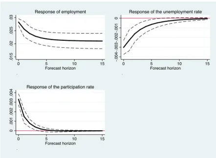
Figure 2 – Impulse response functions in the CEECs .015 .02 .025 .03 0 5 10 15 Forecast horizon . Response of employment -. 0 0 4 -. 0 0 3 -. 0 0 2 -. 0 0 1 0 0 5 10 15 Forecast horizon .
Response of the unemployment rate
0 .001 .002 .003 .004 0 5 10 15 Forecast horizon .
Response of the participation rate
Note : The solid lines are the impulse response functions whereas, the dashed lines represents the 95 percent confidence interval ; Errors are generated with 500 repetitions of Monte Carlo.
5
Results
The figure 2 presents the first impulse response function concerning employment level, unemployment and participation rates, following a one standard error innovation in the employment growth rate. We focus here only on the CEECs group. The level of employment is expected to highlight a long term deviation while the unemployment and participation rates are expected to return to their previous level.
Following the initial spike on employment (upper-left graph), the variable slowly de-creases, reaching a new plateau corresponding to a permanent higher level of employ-ment, around a two percentage points (pp) long term increase. After a fifteen projection simulation, the plateau reached by employment represent 74% of the initial impact (2,1pp against 2,8pp).
We expect a temporary negative reaction of the unemployment rate in the aftermath of a positive drift in employment, while the LFPR is expected to increase. Results are consistent with these predictions and show a 0.3 pp drop in the unemployment rate and a 0.31 pp increase in the LFPR at the moment of the shock. Both variables go back to their long term trajectory. Contrary to Gacs and Huber (2005), the duration of the
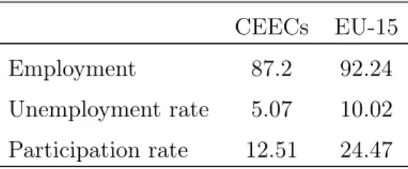
Table 3 – FEVD - Projection after 15 years
CEECs EU-15
Employment 87.2 92.24
Unemployment rate 5.07 10.02 Participation rate 12.51 24.47
Notes : Numbers are expressed in percentage of the total variance and represent the role of the employment variable to explain the variance of the other variable ; Employment shock simulation ; 15 years projection ahead.
unemployment rate response is longer than the participation one. Indeed, the participa-tion rate (on the lower left graph) returns to its long term trajectory within three years. The return of the unemployment rate is slightly higher as it becomes non-significant after five years at a 95% percent confidence interval.
The VAR model allows to decompose the variance of the different forecasted va-riables following the shock. The variance decomposition is an interesting way to ap-prehend to what extend a variable plays a role in explaining the variability of another variable ; this is the forecasted error variance decomposition (FEVD). In the middle-long term (i.e. up to 15 years of projection), the shock on employment explains around 5-to-6% of the unemployment rate variance while it explains 12.5% of the LFPR variance.
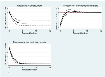
The figure 3presents the impulse response functions for the EU-15 countries, esti-mated after a one standard deviation innovation in employment. The level of employment reaches a long run plateau within five to seven years after the shock ; during this period, around 25% of the initial shock disappears. The response of unemployment and parti-cipation are similar to the previous group. The partiparti-cipation rate goes back to its long term trajectory within five years. The response of the unemployment rate is smaller in duration. Indeed, it takes roughly a decade to fade out.
These results, despite not being identical, are quite similar toDecressin and Fatás(1995) or Beyer and Smets (2015). Nevertheless we find a higher plateau in employment level compared to Beyer and Smets (2015). Indeed, they find a long term employment level corresponding to 50% of the initial shock while we estimate a 75% plateau in the EU-15. Moreover, we observe tighter confidence intervals in case of EU-15 countries. This may be
Figure 3 – Impulse response functions in the EU-15 .01 .012 .014 .016 .018 .02 0 5 10 15 Forecast horizon . Response of employment -. 0 0 4-. 0 0 3-. 0 0 2-. 0 0 1 0 .001 0 5 10 15 Forecast horizon .
Response of the unemployment rate
0 .001 .002 .003 .004 .005 0 5 10 15 Forecast horizon .
Response of the participation rate
Note : The solid lines are the impulse response functions whereas, the grey area represents the 95 percent confidence interval ; Errors are generated with 500 repetitions of Monte Carlo.
justified by a higher cross-section in the EU-15 group, allowing more robust estimation and a more homogeneous average response among the different regions.
But the share of the variance explained by the shock on employment (FEVD) is higher for both the unemployment and the participation in case of the EU-15 group, respectively 10.02 and 24.47 percent. A stronger sensitivity in the EU-15 group reflect a relatively higher level of interconnection between variables upon the labour market.
As we have mentioned earlier, the women labour market participation is an issue in the CEECs as the gap between men and women is increasing while in the EU-15 countries, the distance declined. Following this, it is interesting to look at the previous model, but focusing on the LFPR response separately for men and women. We draw the same model but splitting the participation in two variables. Women and men LFPR are simultaneously introduced to avoid omitted variable bias. According to the IRF’s graphs (left graph on figure 4), following a positive shock on employment, the dynamic of the response seems to be more persistent when looking at the women participation rate in the CEECs compared to the men participation in the same group or to the women participation in EU-15. The shock usually disappears between four to maximum
Figure 4 – Impulse response functions : Women and Men distinction 0 .001 .002 .003 .004 0 5 10 15 Gender IRFs IRF women CEECs IRF women EU15 IRF men CEECs
0 .2 .4 .6 .8 1 0 5 10 15 Standardized IRFs IRF women CEECs IRF women EU15 IRF men CEECs
Note : The lines are the impulse response functions of the participation rate against a shock imposed on employment. This graph compares the reaction between sex and groups of countries, to allow a comparison between the different series. The left graph presents the original IRF while on the right the responses are standardized. The CEECs women participation response is longer in duration
nevertheless, the amplitude of the shock at time t0 is comparable across the two subgroups.
seven years after the innovation. To confirm the higher persistence, we impose the initial shock to unity, (right graph on figure 4). We also draw a mean comparison test to see whether the different series are statistically different and the results corroborates our first impression.
To increase the women participation and to decrease the vulnerability of this fringe of the population, recent IMF and European countries reports point out the necessity to develop the women penetration rate and to invest in childcare programs. Indeed, on average in the EU-15 group, 30-35% of children, less than 3-yo, are engaged in a childcare program. Concerning the CEECs, this rate on average fall below 15% (e.g. in 2016 the ratio in Bulgaria 12.8%, Czech Republic 4.7%, Hungary 15.6%, Poland 7.8%, Romania 17.4%)15.
6
Discussion
The model of Blanchard et al. (1992), described in appendixA, ends up with two mechanisms at stake, following a negative innovation on the labour demand. A change in employment induce wages16 and unemployment to vary over time. A negative shock on employment induces wages to decrease (see eqA.1in appendix A). The wage cut implies firms to migrate, leading to a new creation of employment. This refers to the assumption by which firm location decision depends exclusively on wages (see eqA.4).
On another side, weaker relative wages and higher than average unemployment induce worker net emigration as the opportunity cost of migration decreases.17
Blanchard et al.(1992) formalizes the change in the labour force (denoted by n∗it− n∗it−1) as a function of unemployment and wages (see eqA.3). They interpret this equation like a ‘migration equation’ as worker mobility better explains differences in average employ-ment growth rate compared to differences in the natural population growth rate. The EU adhesion, in 2004 for most CEECs and in 2007 for Romania has led to East-West migration flows which corroborates the author hypothesis. The correlation between the employment growth rate and the natural growth rate of the population is weak (0,054). As we are looking for the dynamics in employment, we have first to disentangle to what extend part-time employment and changes in number of hours worked play a role in employment evolution. The variable we use as "employment" is a headcount measure. It does not consider hours worked such that any change in employment is associated with job creation/destruction. We are aware this tend to minimize effective change in employment as part of variation may be attributed to changes in the number of hours worked. Over the 2000-2016 period, we looked at changes in hours-worked from national accounts statistics and compare them with changes in employment.18 Hours worked, in both groups of countries, do not strictly follow headcount employment. The ratio of hours worked over headcount employment decreased by 2.5 percent in the EU-15 and by 3,5 percent in the CEECs. The drop in this ratio, despite being hard to capture in its impact on the labour market, may be partly analysed through part-time employment.
Using LFS-series, on part-time employment, we find a positive but weak correlation with the employment growth rate. Between 2000/2009 and 2010/2017, part-time ratio increa-sed by 3,7pp in EU15 and by 1,6pp in CEECs expect in Lithuania, Latvia, Poland and
16. In the second part ofBlanchard et al.(1992), the authors introduce relative wages in the model.
The lack of data at the NUTS-2 level does not allow us to implement such a specification.
17. The opportunity cost decreases as the expected income, in the receiving region, increases. The expected income refers to the relative wage times the relative probability of finding a job.
18. Data are extracted from Eurostat website, from the National account series, available from 2000 to 2016. Due to data availability, France, Lithuania, the Netherlands and Poland are excluded.
Romania where it decreases on average by 1,5 pp. We search for a significant relation-ship, regressing part-time ratio on employment. Employment is found to positively and significantly impact the part-time ratio. An increase of one percent in the employment increases part-time ratio by 0.1 percentage point. Regressing only upon the CEECs, the impact is slightly lowered and become non-significant focusing on the period after 2008. Those elements highlight a relatively weak importance of part-time employment changes in the employment behaviour such that, will ignore this channel.
We are aware, informal employment may also influence the dynamics of the response after an employment shock and could explain more persistent responses in the participation rate. According to ILO(2018), the level of informal employment is twice as high in the CEECs, particularly in Poland and Romania, respectively 38% and 28.9%. Drawing the results without theses two countries do not bring any significant change in the partici-pation rate behaviours. The lack on data on this specific topic prevents us from going deeper in this way.
Two main points emerged from our results. The first one concerns the new level of employment after an exogenous labour demand shock, the second lies on the different reactions between the two groups of countries concerning the unemployment and partici-pation rates. When wages increase, following an exogenous positive drift in employment, some firms may reduce their level of employment. This mechanism minimizes the positive impact on employment and justifies the return of the unemployment rate to its long term trajectory. As seen in the previous section, this process needs more time in the CEECs relative to the EU-15.
During the transition, the labour cost represents an important vector of creation of em-ployment. Moreover, a relatively less qualified labour supply will be more easily substitu-ted by physical capital. Thus we would have expecsubstitu-ted a relatively more rapid reaction of firms to employment innovation. Nevertheless, the first part of the transition was followed by wage drop, until they reach a more coherent level with the labour productivity. The stronger resilience of firms to labour cost hike may be explained by a relatively cheaper labour supply. The firm’s wage elasticity seems to be lower than in the EU-15 economies. Moreover, a large pool of unemployed implies a higher bargaining power toward firms to minimize the wage increase after the positive innovation on employment.
Looking at the labour supply, the positive shift in wages and the drop in unemployment, following the employment increase, imply migratory flows to act as an adjustment factor. Indeed inflows of workers induce the participation rate to return to its long term trajec-tory through a wage decrease and unemployment increase. In both group of countries,
the observed participation hikes quickly fade out. The labour force behaviours seem to be similar in both group of countries. We corroborateBeyer and Smets(2015) who high-lighted an increase in geographical flexibility in West Europe labour supply compared to previous studies (Decressin and Fatás,1995). UnlikeGacs and Huber(2005) andFidrmuc
(2004), who found no significant inter-regional labour mobility channel, in the CEECs, our results show an increasing role of the labour force migration.
To disentangle the long term impact on employment we can go through two ex-treme cases. In the first situation, the initial employment shock is fully permanent. Given that the labour demand depends exclusively on wages, this would state that wages, after the impact, do not change at all. As the labour supply depends on wages and unem-ployment, this is only possible if the shock is absorbed by unemployment against wages. Under the assumption by which the unemployment and participation rates returns to their long term trajectory, the decrease in unemployment is offset by workers inflows. On the other side, if the employment shock vanish, given the same assumption as before, this entails a full wage adjustment. Wages absorb the shock such that the level of em-ployment remain the same.
In between, the speed of adjustment of the labour demand and the labour supply will determine the long term impact. Given that labour migration depends on unemployment and wages, while firms mobility depends only on wages, we can state that the more the shock is absorbed by unemployment against wages, the higher the long term impact on employment.
After a fifteen period projection, the employment level remains at three quarters of the initial shock (74,39%) in the CEECs against 67,5% in the EU-15 group. The relatively hi-gher long term impact in the CEECs tends to highlight a relative stronger unemployment channel. Wages adjust less in the CEECs. The relative lower wages’ reaction implies an underlying stronger adjustment of the labour supply. As the participation rate returns to its long term trajectory, the workforce, in the long term is the variable of adjustment. Despite the same mechanism arises in EU-15, the labour supply adjustment is relatively weaker in Western Europe. If the labour supply is seen as the stronger variable of ad-justment in case of a relative high long-term employment impact, then we expect regions with higher than average unemployment rate to suffer from weaker labour supply adjust-ment. Drawing the comparison over the all panel, we find a nine percentage points lower long-term impact on regions with higher than average unemployment rate. This results confirm the intuition upon the speed of the labour supply adjustment.
address the high unemployment issues, found in some left-behind regions, during the first decade of the transition. Unfortunately, our specification gives no information about the distinction between intra-country mobility and international migration. This point is par-ticularly challenging, in the case of the EU development. Macroeconomic policies, turned toward labour force mobility, could induce an increase in regional disparities inducing phenomena like ‘brain drain’ flows at the European level. The way, labour policy mix is drawn in the CEECs is particularly important, given the higher long term potential impact.
7
Conclusion
During the last years, the CEECs were challenged by their labour markets. Between liberalization, privatization, restructuration and economic development, the CEECs do still represent a particular case of access to market economies as they are part of the European Union. Being an EU member implies an increase in EU-members interdepen-dences. The transition was associated with a huge increase in unemployment and a weak mobility amongst regions (Campos and Coricelli,2002).
We replicate the seminal approach proposed by Blanchard et al. (1992) to look at the dynamics of the labour market following a simulated shock on employment. The main purpose of this approach is to disentangle the channel driving labour demand shocks on the employment level, the participation rate and the unemployment rate. Thus it is possible to highlight whether an innovation implies adjustment toward wages or unem-ployment and then to deduce labour demand and supply behaviours.
We draw a comparison between the CEECs and the rest of the EU. We use a reduced model in a panel VAR in order to track the response of the unemployment and participa-tion rates following a shock on employment at the regional level, using NUTS-2 regions. The new plateau reached by employment level represents 75 percent of the initial shock. This tends to highlight a relatively stronger channel toward unemployment instead of wages. The labour supply adjustment is relatively fast compared to the labour labour in both CEECs and EU-15 groups. The long term impact is higher than previously found in the literature likeGacs and Huber (2005) on the CEECs orHalleck Vega and Elhorst
(2016) on the Western Europe.
The participation rate quickly absorbs the employment innovation, reinforcing the role of labour mobility in both sub-groups. The unemployment rate response is longer in du-ration particularly in the CEECs group.
women participation in the CEECs compared to men participation in CEECs but also compared to women participation in the EU-15 group. These results confirm that the women participation is still an issue in the CEECs. The women participation is a double challenge as it has first to be increased to converge to the EU-15 standards but it also has to be less vulnerable to shocks (reducing the persistence of the shock).
The efficient labour supply channel through labour mobility should be carefully analyzed as it may hamper the long term development. If it is associated with a strong increase in regional disparities, then a coherent labour policy mix should be promoted. The re-gional development, thanks to firms attraction, stimulate the local labour market (e.g. investment into infrastructure). Concomitantly, this is possible, if it is associated with a high skilled labour supply (e.g. high education development) and efficient labour market institution to avoid inefficient and useless workforce outflows. All these last points are coherent with the Europe 2020 growth strategy.
Références
Aghion, P. and Blanchard, O. J. (1994). On the Speed of Transition in Central Europe. NBER Macroeconomics Annual, 9 :283–320.
Andrews, D. W. K. and Lu, B. (2001). Consistent model and moment selection proce-dures for GMM estimation with application to dynamic panel data models. Journal of Econometrics, 101(1) :123–164.
Arellano, M. and Bover, O. (1995). Another look at the instrumental variable estimation of error-components models. Journal of Econometrics, 68(1) :29–51.
Beyer, R. C. M. and Smets, F. (2015). Labour market adjustments and migration in Europe and the United States : how different ? Economic Policy, 30(84) :643–682. Blanchard, O. (1998). The Economics of Post-Communist Transition. OUP Catalogue,
Oxford University Press.
Blanchard, O. J., Katz, L. F., Hall, R. E., and Eichengreen, B. (1992). Regional Evolu-tions. Brookings Papers on Economic Activity, 1992(1) :1–75.
Boeri, T. and Scarpetta, S. (1996). Regional mismatch and the transition to a market economy. Labour Economics, 3(3) :233–254.
Boeri, T. and Terrell, K. (2002). Institutional Determinants of Labor Reallocation in Transition. Journal of Economic Perspectives, 16(1) :51–76.
Bornhorst, F. and Commander, S. (2006). Regional unemployment and its persistence in transition countries1. Economics of Transition, 14(2) :269–288.
Boubtane, E., Coulibaly, D., and Rault, C. (2013). Immigration, Growth, and Unem-ployment : Panel VAR Evidence from OECD Countries. Labour, 27(4) :399–420. Campos, N. F. and Coricelli, A. (2002). Growth in Transition : What We Know, What
We Don’t, and What We Should. Journal of Economic Literature, 40(3) :793–836. Commander, S. and Kollo, J. (2008). The changing demand for skills Evidence from the
transition. Economics of Transition, 16(2) :199–221.
Decressin, J. and Fatás, A. (1995). Regional labor market dynamics in Europe. European Economic Review, 39(9) :1627–1655.
d’Albis, H., Boubtane, E., and Coulibaly, D. (2018). International Migration and Regional Housing Markets : Evidence from France. International Regional Science Review, page 0160017617749283.
Eberhardt, M. and Teal, F. (2009). Econometrics for Grumblers : A New Look at the Literature on Cross-Country Growth Empirics.
Eberhardt, M. and Teal, F. (2013). No Mangoes in the Tundra : Spatial Heterogeneity in Agricultural Productivity Analysis*. Oxford Bulletin of Economics and Statistics, 75(6) :914–939.
European Commission and Directorate-General for Employment, S. A. a. I. (2018). Em-ployment and social developments in Europe 2018. OCLC : 1111108637.
Fidrmuc, J. (2004). Migration and regional adjustment to asymmetric shocks in transition economies. Journal of Comparative Economics, 32(2) :230–247.
Gacs, V. and Huber, P. (2005). Quantity adjustments in the regional labour markets of EU candidate countries. Papers in Regional Science, 84(4) :553–574.
Halleck Vega, S. and Elhorst, J. P. (2014). Modelling regional labour market dynamics in space and time. Papers in Regional Science, 93(4) :819–841.
Halleck Vega, S. and Elhorst, J. P. (2016). A regional unemployment model simul-taneously accounting for serial dynamics, spatial dependence and common factors. Regional Science and Urban Economics, 60 :85–95.
Halleck Vega, S. and Elhorst, J. P. (2017). Regional labour force participation across the European Union : a time–space recursive modelling approach with endogenous regressors. Spatial Economic Analysis, 12(2-3) :138–160.
Hansen, L. P. (1982). Large Sample Properties of Generalized Method of Moments Estimators. Econometrica, 50(4) :1029–1054.
Huber, P. (2004). Intra-national labor market adjustment in the candidate countries. Journal of Comparative Economics, 32(2) :248–264.
Huber, P. (2007). Regional Labour Market Developments in Transition : A Survey of the Empirical Literature. The European Journal of Comparative Economics, 4(2) :263–298. ILO (2018). Women and men in the informal economy : a statistical picture. International
Im, K. S., Pesaran, M. H., and Shin, Y. (2003). Testing for unit roots in heterogeneous panels. Journal of Econometrics, 115(1) :53–74.
Jurajda, S. and Terrell, K. (2009). Regional unemployment and human capital in tran-sition economies. Economics of Trantran-sition, 17(2) :241–274.
León-Ledesma, M. A. and McAdam, P. (2004). Unemployment, Hysteresis and Transi-tion. Scottish Journal of Political Economy, 51(3) :377–401.
Love, I. and Zicchino, L. (2006). Financial development and dynamic investment beha-vior : Evidence from panel VAR. The Quarterly Review of Economics and Finance, 46(2) :190–210.
Maddala, G. S. and Wu, S. (1999). A Comparative Study of Unit Root Tests with Panel Data and a New Simple Test. Oxford Bulletin of Economics and Statistics, 61(S1) :631–652.
Marelli, E., Patuelli, R., and Signorelli, M. (2012). Regional unemployment in the EU before and after the global crisis. Post-Communist Economies, 24(2) :155–175. Münich, D. and Svejnar, J. (2007). Unemployment in East and West Europe. Labour
Economics, 14(4) :681–694.
Pesaran, M. H. (2006). Estimation and Inference in Large Heterogeneous Panels with a Multifactor Error Structure. Econometrica, 74(4) :967–1012.
Pesaran, M. H. (2007). A simple panel unit root test in the presence of cross-section dependence. Journal of Applied Econometrics, 22(2) :265–312.
Rios, V. (2016). What drives unemployment disparities in European regions ? A dynamic spatial panel approach. Regional Studies, 0(0) :1–13.
Roodman, D. (2009). How to do Xtabond2 : An Introduction to Difference and System GMM in Stata. The Stata Journal, 9(1) :86–136.
Rutkowski, J. (2006). Labor Market Developments During Economic Transition. World Bank Policy Research Working Paper 3894, World Bank.
Svejnar, J. (1999). Chapter 42 Labor markets in the transitional Central and East European economies. In Handbook of Labor Economics, volume 3, pages 2809–2857. Elsevier.
Todaro, M. P. (1969). A Model of Labor Migration and Urban Unemployment in Less Developed Countries. The American Economic Review, 59(1) :138–148.
Appendices
A
Blanchard et al.
(
1992
) approach
Blanchard et al.(1992) estimate a constant return production function with infinite long run mobility (labour and firms). Initial amenities induce permanent gap in growth rates. While employment rate may change, mobility allows a stable structure for unem-ployment and wages differentials. Each region suffers from idiosyncratic shocks, leading to changes into relative wages and unemployment. Thanks to mobility, employment perma-nently reach a different level. The magnitude of the impact crucially depend on relative speed reaction i.e. how workers and firms react to changes in wages and unemployment. The authors formalizes a labour demand equation. Under full-employment condition :
labour demand : wit= −dnit+ zit
with wit the relative wage, nit the relative employment, zit the position of the labour
demand curve. The indices i and t refer to the regional and temporal dimension. d > 0 reflects the negative slope of labour demand. Full employment assumptions allows n to be given at any point of the time such that a change in z provokes a change in wages. Then movements in z are formalized as :
zit+1− zit= −awit+ xdi+ εdit+1
If a = 0, to a given level of wages, the relative labour demand in a specific region may be characterize by a random walk with drift. a = 0 is too restrictive, firms localisation also depend on wages ; ceteris paribus, relatively weak wages attract firms.
If a > 0, the region is attractive for firms such that xdi induce a drift in demand for
goods and also capture regional amenities. In this case, a is assimilated to the wage short run elasticity. Up to now, it is possible to formalize movements in the labour force, which under the full employment hypothesis are the same as change in employment :
nit+1− nit = bwit+ xsi+ εsit+1
where b is a positive parameter. According to the authors, the most part of the diffe-rence in employment growth rates between regions is attributable to migration flows (i.e. differences in natural population growth rate are considered to be marginal). This hypo-thesis is derived from a high correlation between regional employment growth rate and
migration flow. Thus it is possible to assimilate the previous equation as characterizing migration where xsirepresents the regional amenities (under the hypothesis they are time invariant). wit refers to the link between wages and migration. Given these elements, it
seems reasonable to interpret the parameter b as the short run elasticity of migration to wages. From these three equations, it is possible to derive the relative wage equation :
wit+1= (1 − db − a)wit+ (xdi− dxsi) + (εdit+1− dεsit+1)
with a count for firms mobility while b is turned toward labour mobility (i.e. migration elasticity). If a specific region attract workers, wages should fall ; if the region is more attractive to firms, then wages will increase. We expect relative wages to be different between regions but defined as a stationary process. This point is given by the average relative wage ¯wi = a+db1 xdi−a+dbd xsi. Indeed, the average relative wage does not depend
on time. It is also possible to derive the employment growth rate to get : ∆nit+1= (1 − a − db)∆nit+ (bxdi+ axsi) + (bεdit+1+ εsit+1− (1 − a)εsit)
As before, it is possible to derive the trend in employment growth : ¯ ∆ni = b a + dbxdi+ a a + dbxsi
Under this perspective, while the relative wages follow a stationnary process, an innova-tion on the labour demand/supply permanently affect the level of employment.
The impact of an innovation on the labour demand is given by : ˆ wit= −(1 − a − db)t→ 0 ˆ nit= −b(1 − (1 − a − db)t) (a + db) → −b a + db
A negative innovation on labour demand provoke a drop in short run wages. The different mechanisms at stakes allow wages to go back to the equilibrium (worker migration, employment creation/destruction). The employment speed of adjustment is a function of both short-run and long term elasticities (respectively a and b).
When the full wage adjustment assumption, induced by the full employment hypothesis, is relaxed, unemployment starts playing a role.
cwit= −uit (A.2)
n∗it+1− n∗it= bwit− guit+ xsi+ εsit (A.3)
zit+1− zit= −awit+ xdi+ εdit (A.4)
where n∗it is the log of the labour force19, uitthe unemployment rate defined as the ratio unemployment
employment . The log of employment is then ln(E) = n ∗
it − uit. Labour demand (eq.
A.1) highlights a relation between unemployment and wages under a given labour force. Under equation (A.2), a higher unemployment rate induces a wage cut. Equation (A.3) allow mobility to interact thanks to unemployment and wage (consistent with migration theory (Todaro,1969)).
Last equation (eq A.4) suggests firms location not to be determined by the unemploy-ment rate. A labour demand increase leads to higher wages and a weaker unemployunemploy-ment rate but provoke higher vacancies and longer unemployment durations.
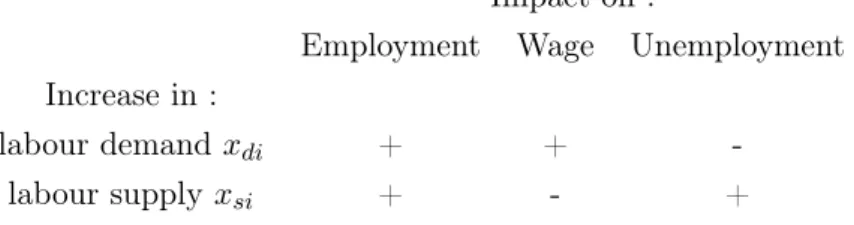
To sum up :
Table 4 – Theoretical expected changes following a positive drift in labour Impact on :
Employment Wage Unemployment
Increase in :
labour demand xdi + +
-labour supply xsi + - +
In the short run, a negative labour demand innovation increases unemployment and induce wage cuts ; in the long term, the effect is opposite thanks to net worker emigration and net inflows of firms. The share of the adjustment attributed to job creation and the share attributed to migration depends on short run elasticities. Given that migration de-pends on unemployment and wages, while firms mobility dede-pends only on wages, implies the following results : the more the shock is absorbed on unemployment against wages, the higher the long term impact on employment.
19. In the previous specification under full employment hypothesis, nitreferred the relative
Table 5 – 1st and 2nd Generation Panel Unit Root Tests CEECs
Employment growth rate
MW (with trend) CIPS (with trend)
χ2/ ¯Zt 799.7 664.1 -15.59 -12.22
p-value 0.00 0.00 0.00 0.00
Employment rate
MW (with trend) CIPS (with trend)
χ2/ ¯Zt 213.1 106.8 -4.070 1.342
p-value 0.00 0.109 0.00 0.910
Participation rate
MW (with trend) CIPS (with trend) χ2/ ¯Z
t 366.7 243.2 -8.286 -4.554
p-value 0.00 0.00 0.00 0.00
EU-15 Employment growth rate
MW (with trend) CIPS (with trend) χ2/ ¯Z
t 2649.3 2229.5 -26.41 -21.93
p-value 0.00 0.00 0.00 0.00
Employment rate
MW (with trend) CIPS (with trend)
χ2/ ¯Zt 714.0 430.3 -3.876 2.515
p-value 0.00 0.024 0.00 0.994
Participation rate
MW (with trend) CIPS (with trend)
χ2/ ¯Zt 1329.7 875.1 -13.00 -5.624
p-value 0.00 0.00 0.00 0.00
Notes : Null for MW and CIPS tests : series is I(1). Maddala-Wu (MW) test assumes cross-section independence. CIPS (Im pesaran Shin) test assumes cross-section dependence is in form of a single
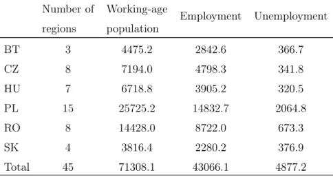
Mandala-Table 6 – Main statistics by country in CEECs group Number of regions Working-age population Employment Unemployment BT 3 4475.2 2842.6 366.7 CZ 8 7194.0 4798.3 341.8 HU 7 6718.8 3905.2 320.5 PL 15 25725.2 14832.7 2064.8 RO 8 14428.0 8722.0 673.3 SK 4 3816.4 2280.2 376.9 Total 45 71308.1 43066.1 4877.2
The three variables are expressed in thousand individuals, on average by country over the 1999-2017 period
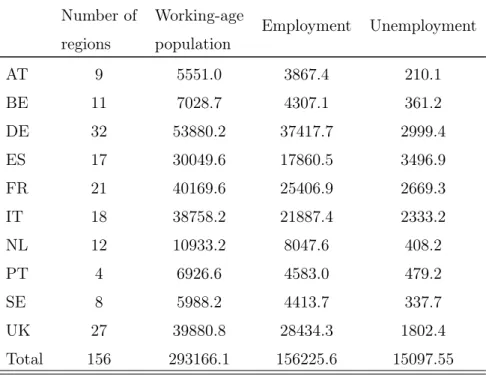
Table 7 – Main statistics by country in EU-15 group Number of regions Working-age population Employment Unemployment AT 9 5551.0 3867.4 210.1 BE 11 7028.7 4307.1 361.2 DE 32 53880.2 37417.7 2999.4 ES 17 30049.6 17860.5 3496.9 FR 21 40169.6 25406.9 2669.3 IT 18 38758.2 21887.4 2333.2 NL 12 10933.2 8047.6 408.2 PT 4 6926.6 4583.0 479.2 SE 8 5988.2 4413.7 337.7 UK 27 39880.8 28434.3 1802.4 Total 156 293166.1 156225.6 15097.55
The three variables are expressed in thousand individuals, on average by country over the 1999-2017 period
Figure 5 – Robustness results .015 .02 .025 .03 0 5 10 15 Employment to Employment Lag = 2 -. 0 0 2 0 .002 .004 0 5 10 15 Employment rate to Employment
Lag = 2
0
.005
.01
0 5 10 15 Participation rate to Employment
Lag = 2 .02 .025 .03 0 5 10 15 Employment to Employment Order 0 .002 .004 0 5 10 15 Employment rate to Employment
Order 0 .002 .004 .006 0 5 10 15 Participation rate to Employment
Order .02 .025 .03 .035 0 5 10 15 Employment to Employment Sub-period 0 .001 .002 0 5 10 15 Employment rate to Employment
Sub-period 0 .001 .002 .003 0 5 10 15 Participation rate to Employment
Sub-period
Notes : To test the robustness of our model, we implement three different specifications. The first set of graphs includes two lags, despite higher confidence interval, the results remain coherent. The second set questions the order in the specification ; once again, results remain unchanged. The last set looks at a sub-panel estimation. To do so, we restrict the two dimensions of our primary CEECs panel. We keep only countries that enter the European in 2004 and are still out of the Euro Area (Czech Republic, Hungary and Poland) and consider only the period from 2004 to 2017 to look at the possible impact of EU adhesion on the labour market. The response functions remain coherent but our confidence intervals sharply increase. In each specification we do not transform our variable such that we have the logarithm of both the employment and participation rates instead of respectively the unemployment rate and the participation rate.