Local magnetic detection and stimulation of neuronal activity

HAL Id: tel-01629395

https://tel.archives-ouvertes.fr/tel-01629395

HAL is a multi-disciplinary open access archive for the deposit and dissemination of sci-entific research documents, whether they are pub-lished or not. The documents may come from teaching and research institutions in France or abroad, or from public or private research centers.

L’archive ouverte pluridisciplinaire HAL, est destinée au dépôt et à la diffusion de documents scientifiques de niveau recherche, publiés ou non, émanant des établissements d’enseignement et de recherche français ou étrangers, des laboratoires publics ou privés.

activity

Vincent Trauchessec

To cite this version:

Vincent Trauchessec. Local magnetic detection and stimulation of neuronal activity. Biological Physics [physics.bio-ph]. Université Paris-Saclay, 2017. English. �NNT : 2017SACLS301�. �tel-01629395�

Local magnetic detection and

stimulation of neuronal activity

Thèse de doctorat de l'Université Paris-Saclay

préparée au Service de Physique de l’Etat Condensé, CEA

École doctorale n°564 Physique de l’Ile de France

Thèse présentée et soutenue à Gif-sur-Yvette, le 4 Octobre 2017, par

Vincent Trauchessec

André Thiaville

Directeur de recherche CNRS

Laboratoire de Physique des Solides, Orsay Président

Nora Dempsey

Directrice de recherche CNRS

Institut Néel, Grenoble Rapporteur

Lauri Parkkonen

Professeur

Aalto University, Helsinki Rapporteur

Claire Baraduc

Directrice de recherche CEA

Spintech, Grenoble Examinatrice

Bruno Le Pioufle

Professeur

Ecole Normale Supérieure Paris-Saclay Examinateur

Myriam Pannetier-Lecoeur

Directrice de recherche CEA

Service de Physique de l’Etat Condensé, Gif-sur-Yvette Directrice de thèse

NNT

:

2

0

1

7

S

A

CL

S

3

01

Ce manuscrit vient conclure mes trois années de thèse au Service de Physique de l’Etat Condensé du CEA. Si elles furent aussi enrichissantes, à la fois sur le plan scientifique et personnel, c’est grâce à toutes les personnes que j’ai pu cotoyer et que je tiens à re-mercier ici.

Je tiens à remercier en premier lieu ma directrice de thèse, Myriam Pannetier-Lecoeur. Grâce à sa confiance, j’ai pu intégrer ce grand projet Magnetrode qu’elle a dirigé durant trois ans. Elle m’a permis d’avoir d’excellentes conditions de travail tout en me lais-sant une liberté très appréciable au quotidien. Je lui suis également très reconnaislais-sant d’avoir pu profiter de la dimension internationale qu’elle a donnée à ma thèse, à travers plusieurs missions qui rendraient jaloux plus d’un thésard (Helsinki, Lisbonne, Franc-fort, Marseille, Séoul, Dublin, etc...)!

Je remercie également le directeur du groupe LNO, Claude Fermon, dont les com-pétences scientifiques remarquables couvrent un spectre aussi large que celui reliant la physique fondamentale à l’ingénierie. Ses conseils et ses idées novatrices ont été un atout considérable pour l’avancement de cette thèse.

J’ai aussi eu la chance de travailler avec d’autres étudiants qui ont participé à faire avancer ce projet. Tout d’abord, Laure Caruso, première thésarde à se lancer courageuse-ment dans la fabrication de magnetrodes et avec qui j’ai eu le plaisir d’interagir pen-dant un peu plus d’un an. Puis Josué Trejo-Rosillo, post-doc durant un an, dont les compétences en instrumentation furent très précieuses. Deux stagiaires de master ont également participé au projet, Jocelyn Boutzen sur la "délicate" découpe laser, et Chloé Chopin, récemment promue thésarde, grâce à qui ce travail ira j’en suis sûr bien plus loin.

Je tiens à remercier Elodie Paul, spécialiste microfabrication, dont l’aide m’a per-mis de gagner beaucoup de temps, que ce soit durant les process ou avec KLayout.

Solignac pour tous nos échanges et tout le temps qu’elle m’a consacré, en particulier durant la phase de rédaction puis de préparation de la soutenance. Merci à Jean-Yves Chauleau, nouvelle recrue du LNO, toujours prêt à discuter physique ou autre, autour d’un café ou plutôt d’une bière. J’ai aussi une pensée pour Corinne Kopec-Coelho pour sa disponibilité et parce qu’elle m’a largement facilité les tâches administratives pour chaque mission. Je remercie également le directeur du SPEC, François Daviaud, pour avoir pris le temps de faire avec moi des points réguliers sur ma thèse et ma situation personnelle.

Tous les résultats présentés dans cette thèse n’auraient pas vu le jour sans le tra-vail de nos collaborateurs neuroscientifiques. Interagir avec eux fut très enrichissant et m’a permis d’aborder la compléxité d’un système biologique avec un recul et une hu-milité indispensables. Tout d’abord, les dizaines de tentatives et le nombre d’heures incalculables passées à essayer de mesurer ce signal biomagnétique furent récompen-sées grâce à la persévérance et à la rigueur de l’équipe composée de Gilles Ouanounou, Francesca Barbieri, Apostolis Mikroulis, Thierry Bal et Alain Destexhe. Je remercie égale-ment l’équipe du Professeur Pascal Fries pour leur professionnalisme et leur enthousi-asme durant ces mémorables expériences in vivo: Thomas Wunderle, Chris Lewis, Jian-guan Ni, et en particulier Patrick Jendritza pour avoir eu, au milieu de la seconde nuit, cette idée lumineuse du montage qui a finalement permis la toute première mesure magnétique intracorticale de spikes.

Enfin je remercie les membres du jury qui ont accepté d’examiner ce travail de thèse: André Thiaville, Nora Dempsey, Claire Baraduc, Bruno Le Pioufle, et en parti-culier Lauri Parkkonen, dont l’impressionnante culture et rigueur scientifique m’ont permis de peaufiner ce manuscrit dans les moindres détails.

Je pense également à tous mes collègues qui ont rendus ces trois années de thèse très agréables. Que ce soit les grands anciens du laboratoire: Camille, Pierre-André, Christian, Sylvio; l’équipe du midi avec qui chaque repas se passe dans la bonne humeur: mon parrain Yannick, les incollables du classement ATP Grégoire, Michel et Jean-Baptiste, les GMT; les membres de Crivasense: Amal, Paolo, Yann, Raphaël, Florian, Maxime; et tout ceux avec qui j’ai pu partagé de bons moments au SPEC ou sur un terrain de foot: Sebastian, Matthieu, Maëlle, Chloé, Marc, Reina, Fawaz, Julien, Andrin, Théophile, Stefan, Nathanaël, Li, Xavier, Anaëlle, Bastien, Romain, Daniela, Bartolo, Fernanda,

Néanmoins, je ne serais pas arrivé jusqu’ici sans avoir croisé la route de quelques brillants professeurs. Je me dois de citer l’excellente équipe de prépa ATS du lycée La Fayette de Clermont-Ferrand, à qui je dois la large majorité de mes quelques connais-sances scientifiques, et sans qui je n’aurais jamais atteint l’ENS: Bruno Abadie, Em-manuel Hehunstre, Christophe Pierre, Jean-François Planeix, Philippe Josselin, et Marie-Christine Lesprit. A Cachan, les cours de Arnaud Bournel, Sylvie Retailleau, Jean-Pierre Barbot, furent également passionnants, et j’ai eu la chance d’intégrer mon premier lab-oratoire sous la direction de Damien Querlioz, avec qui j’ai pris beaucoup de plaisir à faire de la recherche pour la première fois, et dont les qualités scientifiques lui as-sureront une carrière déjà brillante.

Enfin, je remercie tous mes amis pour m’avoir fait penser à autre chose que cette thèse durant ces trois ans, ma famille, ma soeur Valérie, grâce à qui j’étais dans les meilleures conditions pour réussir l’année déterminante de classe prépa, mes parents, qui m’ont depuis toujours encouragé à poursuivre dans la voie scientifique, ma belle-famille, grâce à qui j’ai pu notamment peaufiner ce manuscrit à l’ombre d’oliviers gar-dois, et enfin Valentine, pour tout son soutien quotidien sans faille. Merci à tous!

L’activité cérébrale se traduit par des courants ioniques circulant dans le réseau neuronal. La compréhension des mécanismes cérébraux implique de sonder ces courants, via des mesures électriques ou magnétiques. Pour cela, différents out-ils de mesure ont été développés, couvrant une échelle spatiale qui s’étend sur plusieurs ordres de grandeurs, de la dizaine de nanomètres à la taille d’une aire cérébrale. Le comportement d’un neurone est bien identifié grâce aux techniques d’électrophysiologie traditionnelles, du type micro-électrodes ou patch-clamp. A l’échelle du cerveau, les techniques d’imagerie non-invasives permettent de cartogra-phier les différentes régions et leurs fonctions associées. La méthode la plus simple est l’électroencéphalographie (EEG), qui consiste à placer des électrodes directement sur le cuir chevelu du patient afin d’enregistrer les variations de potentiel électrique. Sa facilité de mise en oeuvre fait de l’EEG une technique largement répandue dans les hôpitaux et les centres de recherche. Cependant, la résolution spatiale est particulière-ment faible: le nombre de neurones corticaux présents dans la zone couverte par la surface d’une électrode de 1 cm2est d’environ 107. De plus, si cette technique présente l’avantage d’être non-invasif, les ions déplacés par l’activité neuronale doivent se propager à travers plusieurs tissus (méninges, crâne, cuir chevelu) présentant des propriétés différentes avant d’atteindre l’électrode, ce qui rend le signal EEG sensible à la distorsion et au filtrage. A cette activité électrique est associé un champ magné-tique, détectable de façon non-invasive par des capteurs ultra-sensibles. L’activation synchrone d’une population de neurones génère un champ magnétique de quelques 10−13T à une distance de l’ordre de 3 cm. Cette technique, la magnétoencéphalo-graphie (MEG), est basée sur l’utilisation de SQUIDs (Superconducting QUantum Interference Devices). Ces capteurs, constitués d’une boucle supraconductrice et de deux jonctions Josephson, atteignent des sensibilités de l’ordre de 10−15 T/pHz. Les systèmes MEG possèdent jusqu’à 306 SQUIDs qui permettent une localisation des sources plus précise que l’EEG. En effet, la perméabilité des tissus étant égale à celle du vide, le champ magnétique se propage des neurones jusqu’aux capteurs sans le moindre effet de filtrage ou de distorsion. Le signal MEG est simplement

source-capteur comprise entre 3 et 5 cm. Des études récentes ont montré la faisabilité de mesures MEG basées sur des magnétomètres atomiques. Ne nécessitant pas de système cryogénique, ces magnétomètres peuvent être positionnés directement sur le cuir-chevelu. Les champs magnétiques enregistrés atteignent alors 10−12T. Cepen-dant, il n’existe pas d’outils permettant de mesurer localement le champ magnétique à l’intérieur du cortex, de la même manière qu’une micro-électrode insérée au sein du réseau neuronal donne accès aux variations locales du potentiel électrique. Un tel outil de magnétophysiologie présenterait plusieurs avantages. Tout d’abord, une électrode conventionnelle traduit une quantité scalaire, le potentiel électrique, dû aux variations du nombre de charges présentes autour de son extrémité, indépendamment de leurs directions de propagation. Un capteur de champ magnétique fournit une quantité vectorielle, contenant deux informations: l’intensité des courants ioniques ainsi que leurs directions de propagation. Cette information simplifierait grandement la reconstruction de la configuration géométrique de la zone sondée. De plus, tout comme le signal MEG, le champ magnétique mesuré localement traverse les tissus et le milieu conducteur environnant sans subir de distorsion. La mesure locale permettrait également de faciliter l’interprétation du signal MEG enregistré à l’échelle cérébrale. Enfin, le champ magnétique émit par un neurone lors de l’émission d’un potentiel d’action permettrait de remonter au courant axial le long de l’axone sans être en contact direct avec la cellule. Toute ces perspectives nécessitent le développement de capteurs magnétiques à la fois suffisamment sensibles pour être capable de détecter le champ magnétique généré par les courants neuronaux (de l’ordre de 10−9 T), dont la géométrie est miniaturisable aux dimensions des cellules, et fonctionnant à température ambiante. C’est l’objet de cette thèse, organisée de la façon suivante.

Le premier chapitre présente l’état de l’art des mesures de l’activité neuronale, en mettant l’accent sur les mesures magnétiques. A l’échelle cérébrale, les techniques d’imagerie dites structurelles (Imagerie par Résonance Magnétique) et fonctionnelles (IRM fonctionnelle, Tomographie par Emission de Positons (TEP), EEG, MEG) perme-ttent d’obtenir des cartographies de l’activité cérébrale avec différentes résolutions spatiales et temporelles. Les techniques d’IRMf et TEP sont dites hémodynamiques: l’activité des cellules augmente la consommation d’oxygène, entrainant localement un flux de sang plus important. Les propriétés magnétiques de l’hémoglobine dépendant de la quantité d’oxygène transportée, ce flux génère un signal dit BOLD (Blood-Oxygen-Level Dependent) détectable par IRMf. Cependant, la résolution temporelle

ailleurs, détecter le champ électromagnétique émis par les neurones donne une vision directe et quasi-instantanée de l’activité cérébrale, avec une résolution temporelle de l’ordre de la milliseconde. Afin d’interpréter les signaux enregistrés par les techniques d’EEG et MEG décrites précédemment, les mécanismes de génération et de trans-mission du signal électrique entre neurones sont décrits. Deux principales sources de champ magnétique peuvent être identifiées: les courants dus à la propagation du potentiel d’action et les courants post-synaptiques. Ces courants post-synaptiques représentent la contribution la plus forte sur les signaux EEG/MEG, du fait notam-ment de leur plus grande extension temporelle, quelques dizaines de millisecondes, augmentant ainsi l’effet global de sommation. La détection de potentiel d’action n’est possible que via des outils d’électrophysiologie, dont la partie sensible est positionnée soit à l’intérieur du neurone actif (enregistrement intra-cellulaire) soit dans le milieu extérieur, afin de mesurer les potentiels d’actions de la population de neurones proches de l’électrode (enregistrement extra-cellulaire). La signature magnétique d’un potentiel d’action n’a été mesurée que dans des systèmes biologiques simples (axone géant de calmar ou d’écrevisse, muscle squelettique, ver), via l’utilisation de SQUIDs, de bobine d’induction, ou plus récemment de magnétomètre à centres NV. Les capteurs développés dans cette thèse sont basés sur un effet quantique dit de magnétorésistance géante. Leur principe de fonctionnement, leur fabrication et leurs performances sont décrits dans le second chapitre.

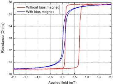
L’effet de magnétorésistance géante fut découvert expérimentalement par A. Fert et P. Grünberg en 1988. L’expérience pionnière montre que la résistance électrique de multi-couches Fer/Chrome varie de 80% entre les états d’aimantation parallèles et anti-parallèle de deux couches adjacentes. A partir de cette découverte, B. Dieny et S. Parkin développèrent un nouveau type de capteur magnétique, la vanne de spin. Ces vannes de spin, ou capteurs GMR, sont constituées d’une couche d’un matériau magnétique à haute coercivité (couche dure) et d’une couche d’un matériau magné-tique à faible coercivité (couche libre) séparées par un espaceur non-magnémagné-tique. En présence d’un champ magnétique extérieur, la couche libre alignera son aimantation avec celui-ci, alors que la couche dure conserva la même direction d’aimantation, ce qui entrainera une variation de la résistance globale du dispositif. Afin d’obtenir une variation linéaire de la résistance en fonction du champ magnétique appliqué, le design de la vanne de spin est choisi de façon à ce que les aimantations de la couche libre et la couche dure soient perpendiculaires à champ nul. Pour les structure de

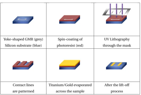
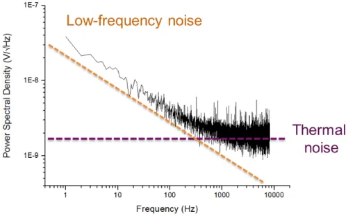
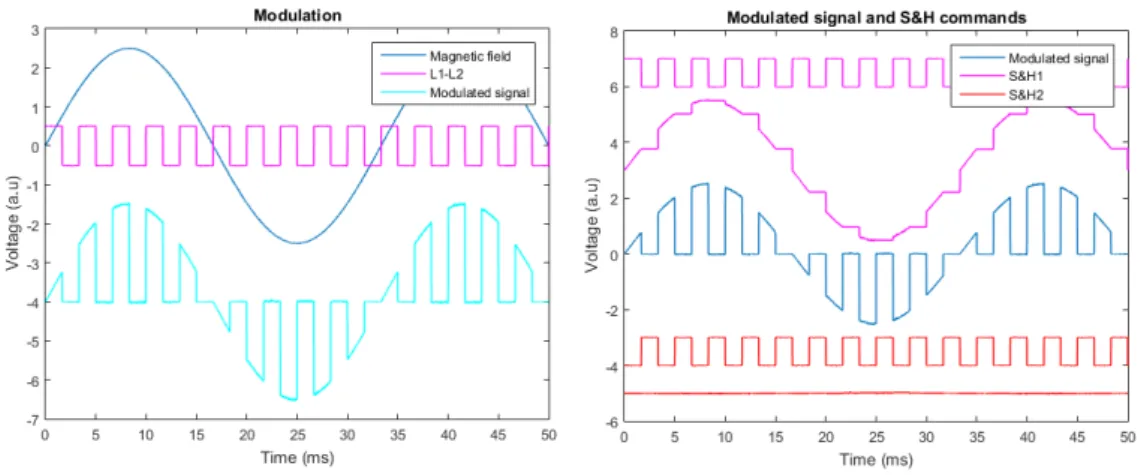
aimant dit de bias permet d’orienter la couche libre dans la direction souhaitée. Dans les deux cas, la forme de la vanne de spin est obtenue par gravure sèche à l’Argon après une étape de lithographie UV. La vanne de spin est ensuite contactée électriquement via des lignes de Titane/Or déposées par évaporation (150 nm), puis le capteur est passivé par pulvérisation d’une bicouche d’alumine et de nitrure de silicium (300 nm). Les capteurs sont ensuite découpés par gravure ionique réactive profonde, afin de les libérer du substrat de silicium de 200 micromètres d’épaisseur. Chaque capteur est ensuite collé sur un circuit PCB et testé afin de déterminer sa sensibilité et son niveau de bruit. Les sensibilités typiques sont comprises entre 2 %/mT et 20 %/mT selon la taille de la vanne de spin, tandis que les niveaux de bruit sont de l’ordre de 1 nT/pHz à 1 kHz. Dans la bande de fréquence inférieure [1 Hz - 1 kHz], la composante de bruit dominante est celle du bruit dit en 1/f. Une technique de modulation fut développée durant cette thèse afin de réduire ce bruit basse fréquence et ainsi augmenter la détec-tivité des capteurs dans cette bande de fréquence d’intérêt central en neuroscience.

Le troisième chapitre présente une expérience in vitro de mesure du champ magnétique généré par un potentiel d’action basée sur des capteurs GMR. Ces mesures ont été réalisées en collaboration avec l’équipe UNIC (Unité de Neurosciences, Infor-mation et Compléxité) du CNRS. Le système biologique choisi est le muscle soléaire de souris, qui présente beaucoup de caractéristiques favorables à une première validation de ce genre de mesure. Il est constitué d’environ 800 fibres musculaires alignées parallèlement, innervées chacune en leur centre par une seule synapse excitatrice. Le potentiel d’action est déclenché dans le nerf par une impulsion électrique puis se propage jusqu’à la jonction neuromusculaire au centre du muscle et génère deux potentiels d’action se propageant symétriquement vers les deux extrémités. Les courants axiaux générés par la propagation de ces potentiels d’action génèrent un champ magnétique détectable en positionnant le muscle sur des capteurs GMR dont le design est adapté à la taille du système (1 mm * 10 mm). Les signaux magnétiques enregistrés représentent une variation biphasique de 2,5 nT d’amplitude sur une durée d’environ 4 ms. Ces courbes ont été obtenues après un moyennage sur 500 stimulations et présentent un rapport signal sur bruit de l’ordre de 10. Trois mesures de contrôles ont permis de vérifier la véracité de ces enregistrements. Tout d’abord, la même mesure fut réalisée en coupant le courant d’alimentation de la vanne de spin. Ainsi, toute variation de résistance dûe à un champ magnétique est supposée disparaître, contrairement à un artefact dû au couplage capacitif à travers la solution

champ magnétique ne soient plus orientée selon la direction de sensibilité de la vanne de spin. Enfin, une dernière vérification fut mise en oeuvre en mesurant le signal après avoir injecté une dose de curare dans le bain afin de bloquer la propagation du potentiel d’action au niveau de la jonction neuromusculaire. Dans les trois cas, ces expériences furent concluantes, permettant d’affirmer respectivement que le signal mesuré est bien dû à un champ magnétique, créé par des courants axiaux le long des fibres musculaires, eux-mêmes dûs à la propagation du potentiel d’action. Par ailleurs les modèles théoriques développés sont en accord avec les mesures expérimentales, suggérant notamment que près de 75% du champ magnétique généré par les courants axiaux est écranté par les courants de retour dans le milieu extra-cellulaire. Toute cette étude valide l’utilisation de capteurs GMR pour la mesure de signaux biomagnétiques et fut publiée dans Scientific Reports.

Le quatrième chapitre est consacré aux mesures in vivo réalisées dans le cortex visuel de chats et présente les premières signatures magnétiques intra-corticales de potentiels d’action. Ces mesures ont été réalisées en collaboration avec le groupe du Professeur Pascal Fries de l’Ernst Strüngmann Institute de Francfort. Pour cela, des capteurs GMR de (3µm*50µm) ont été déposés à l’extrémité de pointes d’une finesse et d’une épaisseur de 200µm, afin d’obtenir l’équivalent magnétique des électrodes traditionnelles. Ces magnetrodes doivent être suffisamment robustes pour résister à l’insertion dans le cortex, et suffisamment fines pour créer le moins de dommage possible au niveau des neurones corticaux. Une électrode de tungstène est placée sur la magnetrode de façon à mesurer le potentiel local au plus près du capteur GMR. La pointe est insérée dans le cortex visuel, dont la profondeur est de l’ordre de 1,6 mm, puis une stimulation visuelle est appliquée durant 1 seconde via un écran placé face au chat. La stimulation génère une augmentation de l’activité neuronale dans le cortex visuel, facilement mesurable électriquement par l’électrode placée dans le milieu extra-cellulaire. Le nombre de potentiels d’action enregistrés passent de 30 spikes/sec à environ 200 spikes/sec. Un enregistrement typique correspond à 1000 stimuli de 1 seconde, séparés par un délai de 2 secondes et d’un délai aléatoire pour éviter l’adaptation neuronale. Le traitement des données enregistrées permet ensuite d’extraire le signal magnétique de la façon suivante. Chaque spike enregistré par l’électrode est assez facilement extractible grâce à un bon rapport signal sur bruit. Environ 40 000 spikes sont ainsi extraits selon leur polarité positive ou négative, centrés sur une fenêtre de 10 ms, puis moyennés. Le spike moyen présente une amplitude

ces acquisitions permet de diminuer le bruit d’un facteur 200, pour atteindre environ 0,4 nT. Un signal magnétique de 1,2 nT d’amplitude, durant 0.4, msapparaît alors clairement hors du bruit. Ce signal magnétique change également de polarité lorsque la polarité des spikes électriques s’inverse. Son origine magnétique est confirmée par le même contrôle que lors des expériences in vitro: lorsque le courant dans le capteur est nul, le signal magnétique disparait. Ce résultat représente la première mesure magnétique in vivo intra-corticale de potentiels d’action. Cependant, ce résultat pose plusieurs questions et ouvre beaucoup de perspectives: sachant que la modélisation est beaucoup plus complexe que le modèle du muscle squelettique présenté précédemment, il est difficile de prévoir l’amplitude et la durée du signal. Le nombre de neurones participant à ce signal est également difficile à estimer, étant donné la distribution continue de l’amplitude des spikes mesurés. Néanmoins, des avancées peuvent être réalisées à plusieurs niveaux: la sensibilité des capteurs peut être augmentée en utilisant le phénomène de magnétorésistance tunnel (TMR) et en réduisant leur bruit basse fréquence par la technique de modulation présentée au chapitre 2. Des magnetrodes comportant plusieurs vannes de spin (ou TMR) et plusieurs électrodes intégrées le long de la pointe permettront de faire des mesures laminaires dans la profondeur du cortex et d’avoir une cartographie des potentiels et des courants bien plus précise. Par ailleurs, une mesure simultanée du signal magné-tique local via des magnetrodes et du signal magnémagné-tique mesuré en MEG via un SQUID permettrait d’affiner la résolution du problème inverse. Enfin, une micro-bobine pourrait être intégrée sur la pointe de la magnetrode et ainsi stimuler localement une population de neurones via des impulsions de champ magnétique. Ce projet a été abordé au début de cette thèse et fait l’objet du dernier chapitre.

Ce cinquième et dernier chapitre de cette thèse présente les travaux dont l’objectif était de stimuler localement une population de neurones via une impulsion de champ magnétique. Si la stimulation électrique est aujourd’hui largement utilisée pour le traitement de maladies neurodégénératives, elle présente plusieurs inconvénients (faible contrôle des champs électriques, inflammation des tissus, rejet de l’électrode par la cellule). La stimulation magnétique s’affranchit de ces effets mais cette solution n’a été mise en œuvre qu’à l’échelle cérébrale, par la stimulation transcrânienne (TMS). L’objectif est de développer des micro-inducteurs capables de générer un champ élec-tromagnétique suffisamment important pour induire une réponse des quelques neu-rones ciblés. Les travaux présentés jusqu’à présent dans ce domaine mettent en œuvre

groupe a fait état, en 2012, de stimulation magnétique à une échelle micrométrique, en utilisant des inducteurs de 500µm de diamètre. Un code de simulation numérique pour étudier l’influence des différents paramètres (rayon, longueur, nombre de spires), ainsi que pour calculer les champs créés dans tout l’espace en s’adaptant à la géométrie des inducteurs fabriqués a été développé. En collaboration avec le groupe UNIC du CNRS, une première expérience de stimulation in vitro sur une tranche d’hippocampe a été mise en place. Cette expérience consiste à placer la bobine, de 5 mm de rayon, au plus près des neurones, tout en enregistrant électriquement leurs réponses via une électrode plongée dans le milieu extra-cellulaire. Les neurones étant sensibles unique-ment au champ électrique, il est nécessaire de fournir des impulsions de courant générant un champ magnétique variable pour engendrer des courants induits dans le milieu cellulaire. Pour cela un condensateur de grande capacité est déchargé directe-ment dans la micro-bobine. Ces impulsions génèrent à la fois un artefact de stimula-tion mesuré par les électrodes ainsi qu’un artéfact dû aux vibrastimula-tions de la bobine du-rant la décharge. Les dernières expériences donnent plusieurs pistes d’amélioration du système, afin notamment de s’affranchir des artéfacts et de mesurer en temps réel l’évolution du potentiel de membrane d’un neurone soumis à la stimulation magné-tique locale.

Contents xv

Introduction 1

1 Brain Imaging and Magnetophysiology 9

1.1 Large-scale brain imaging . . . 10

1.1.1 Basics of brain imaging . . . 10

1.1.1.1 Structural imaging . . . 10

1.1.1.2 Functional imaging . . . 11

1.1.2 Magnetoencephalography . . . 13

1.1.2.1 Magnetic fields of the brain. . . 13

1.1.2.2 MEG with SQUIDs . . . 18

1.1.2.3 Future developments . . . 21

1.2 Local-scale neuronal sensing . . . 25

1.2.1 Theoretical framework. . . 25 1.2.1.1 Circuit neuroscience. . . 25 1.2.1.2 Conventional electrodes . . . 25 1.2.1.3 Advantage of magnetometry . . . 27 1.2.2 NV centers . . . 28 1.3 Conclusion . . . 32 2 Magnetoresistive sensors 41 2.1 Theoretical basis . . . 43 2.1.1 Origin of spintronics . . . 43 2.1.2 Stern-Gerlach experiment. . . 43 2.2 Magneto-resistive sensors . . . 44 2.2.1 Anisotropic magneto-resistance . . . 44 2.2.2 Giant magneto-resistance . . . 45

2.3 Sensor microfabrication process . . . 49 2.3.1 Stack deposition . . . 49 2.3.2 Probe design. . . 51 2.3.3 Photo-Lithography . . . 52 2.3.4 Etching . . . 53 2.3.5 Deposition techniques. . . 53

2.3.6 Cutting of the sample . . . 55

2.3.6.1 Deep-RIE . . . 56 2.3.6.2 Laser cutting . . . 56 2.4 Performance of GMR sensors . . . 58 2.4.1 Magneto-transport . . . 58 2.4.2 Noise . . . 59 2.4.2.1 Noise sources . . . 59 2.4.2.2 Measurement setup . . . 61

2.5 Low-frequency noise canceling . . . 64

2.5.1 State of the art. . . 64

2.5.2 Theoretical principle . . . 65

2.5.3 Custom-made sensors . . . 66

2.6 Conclusion. . . 70

3 In-vitro magnetic action potential in skeletal muscle 75 3.1 Theoretical framework . . . 76

3.1.1 Magnetomyography (MMG) . . . 76

3.1.2 Nerve-Muscle features . . . 77

3.2 Electrophysiology . . . 79

3.2.1 Action potential dynamics. . . 79

3.2.2 Results . . . 80

3.3 Modeling . . . 84

3.3.1 Features of the model . . . 84

3.3.2 Results . . . 85 3.4 Custom-made GMR sensor . . . 89 3.4.1 Micro-fabrication . . . 89 3.4.2 Performance. . . 90 3.5 Magnetic recordings . . . 94 3.5.1 Experimental setup. . . 94 3.5.2 Results . . . 94

3.5.2.2 Control experiments . . . 98

3.6 Conclusion . . . 100

4 In-vivo magnetic action potential in visual cortex 105 4.1 Theoretical framework . . . 106

4.1.1 Visual cortex. . . 106

4.1.2 Local Field Potential (LFP). . . 108

4.1.3 Spiking activity . . . 110 4.2 Magnetrode . . . 113 4.2.1 Microfabrication . . . 113 4.2.2 Difficulties encountered . . . 119 4.2.3 Performance. . . 120 4.3 Experimental setup . . . 122 4.3.1 Biological procedures . . . 122 4.3.2 Technical features . . . 122 4.4 Results . . . 124

4.4.1 Local field potentials . . . 124

4.4.2 Magnetic spikes. . . 129

4.5 Conclusion and perspectives . . . 145

5 Local magnetic stimulation 151 5.1 Transcranial Magnetic Stimulation (TMS) . . . 152

5.1.1 Early development . . . 152

5.1.2 Basic principles . . . 153

5.2 Local Magnetic Stimulation (LMS) . . . 155

5.2.1 Motivations . . . 155

5.2.2 LMS setup . . . 157

5.2.3 Experiments . . . 160

5.3 Conclusion . . . 165

La culture, c’est ce qui répond à l’homme quand il se demande ce qu’il fait sur terre.

André Malraux

Understanding the genesis of our intellectual faculties and of our emotions is one of the most challenging tasks for scientists to take up. This ambitious goal can only be achieved by bridging gaps between different areas of science. The various backgrounds of neuroscientists, clinicians, physicists, and engineers span a diversity of approaches, and connecting them efficiently is of key importance to achieve major breakthroughs.

Research in electroencephalography (EEG) and magnetoencephalography (MEG) illustrates very well this point. There is a need to overcome the barriers that stand in the way of a fruitful communication between a physicist and a prospective physiolo-gist. However, both have to deal with a very complex inhomogeneous system, where non-linear processes unfold. While the first is used to describe physical phenomena with concise equations, the latter takes advantage of a large amount of data output to develop models in the light of experiments. Even if physics is in essence an experimen-tal science, the theoretical framework leading to perform an experiment often needs to be clearly defined. Fortunately, EEG and MEG specialists have not always followed this path. They have been able to carry out groundbreaking experiments without a prior complete modeling exercise. A relevant example is the observation of spontaneous ac-tivity, such as alpha rhythm (8 - 13 Hz) present in a subject with eyes closed, or the de-tection of epileptic seizures. Anyway, scientists are striving more than ever for improved tools to measure brain activity. This great enthusiasm will certainly persist, until light is shed through what Paul Nunez [9] calls the window on the mind.

This thesis aims at providing one of these tools. A wide range of techniques to record electrical activity are successful, spanning from the micro-scale (single ion channel), to

the meso-scale (Local Field Potential), up to the brain macro-scale (EEG). Current sen-sors used in MEG are very sensitive but cannot be miniaturized. Moreover, they operate at a very low temperature, which is prohibitive for any contact with living tissue. These are the main reasons why biological magnetic fields have not been measured at the neu-ronal scale so far. Yet, having a magnetic counterpart of the traditional micro-electrode would represent a step forward towards the investigation of local sources of neuronal magnetic activity.

Before embarking on such a project, it is definitely essential to analyze the path that was taken by scientists since the very early times. To build this technology up, we benefited from a deep understanding of the principles of electromagnetism, developed during the XIX century, and also from the more recent discoveries in quantum physics. If the brain is still fascinating people nowadays, it is worth noting that the attraction between two magnets was also considered as a mysterious phenomenon for centuries. The major steps taken over two thousand years are described below. Assessing how far we have come, from considering magnetism as a divine power to the rigor of Maxwell’s equations, might be an example for other areas of science.

The discovery of magnetism is lost in the past of Ancient Greece, but the earliest known mention is attributed to Thales of Miletus (-625 BC ; -546 BC). The attraction be-tween naturally magnetized pieces of magnetite, called lodestone, and small pieces of iron has fascinated Thales and many philosophers like Plato (-428 ; -348), Aristotle (-384 ; -322) and Lucretius (-99 ; -54). Magnetite is a ferrimagnetic mineral that forms during volcanic eruption when liquid iron gets oxidized in contact with air. Its remanent mag-netization is caused by the Earth’s magnetic field that polarizes the stone throughout its cooling. Lucretius, in De Natura Rerum, confirmed that the name "magnetite" was attributed in reference to Magnesia, a city that owes its name to Magnes, son of Zeus and Thyia.

Following this golden Hellenic era, it took several centuries until a renewed scien-tific interest. The french Pierre de Maricourt wrote in 1269 the first treaty describing the laws of magnetic attraction and repulsion, Epistola de magnete. As a military engineer, he was obviously interested in the issues of compass, a strategic tool of key importance for the navy. The work of de Maricourt was acknowledged by the one who stands as one of the pioneer of experimental science, William Gilbert. He published De Magnete in 1600, after twenty years of various experiments. He set himself the objective to remove any doubts concerning magnetic phenomena, especially chasing all the superstitions

which prevailed at the time. Plenty of experiments on a sphere-shaped magnet led him to conclude that the Earth was itself a magnet, and deduced why the compass needle points directly at the north pole. He was also able to separate the electrostatic attraction of amber from the magnetic attraction of lodestones, laying out the very first electricity basics.

Despite the success of Gilbert’s work, the main obstacle in the development of a complete electromagnetic theory was the lack of a continuous source of electricity. The triggering event that led the physicist Alessandro Volta to the discovery of the voltaic pile was a lively debate with a... biologist! Luigi Galvani, anatomist at the university of Bologna, published De viribus electricitatis in moto musculari in 1791. He had ob-served that the contact between his scalpel and the crural nerve of a dead frog induced a contraction, at the exact moment when an electric spark was generated in close vicin-ity. Amazed by this fortuitous event, Galvani shifted the experiment on the roof of his house to check the twitch response of the muscle being struck by lightning. The experi-ment met his expectations, but, more importantly, he discovered that the mere contact between the copper hook, connected to the spinal cord, and the iron balustrade in-duced the same response without any lightning bolt. After this finding, Galvani coined the term "animal electricity". However, Volta was convinced that the electric source was not the muscle, but was generated by the contact between the two different metals. His will to rule out the theory of Galvany led him to produce, in 1800, a stack of copper and zinc discs, on top of each other, separated by a layer of cardboard soaked in saline water. This invention, still known as the voltaic pile, provided scientists a continuous stable current source, giving rise to the upcoming electromagnetic revolution.

The starting gun was fired in 1820 in Copenhagen. Hans Christian Oersted, a Dan-ish physicist, was giving a lecture on electricity at the University. Switching on a battery to supply a circuit, he noticed that the compass needle deflected from the North pole when current was flowing through the wire. The providential circumstances of this dis-covery has been disputed; anyhow, the intimate relation between electricity and mag-netism was demonstrated for the very first time. Beyond the tremendous impact of this discovery, it was the first ever example of the conversion of electrical energy to mechan-ical energy, which is still largely present in our daily life. Oersted’s experiment spread over Europe, especially in France, after being presented to the Academy of Sciences by Francois Arago. One of his colleague, André Marie Ampère, a brilliant mathematician, promptly took charge of this issue that just begged to be formalized. Besides, Ampère demonstrated the equivalence between a magnet and a solenoid supplied by an

elec-tric current. Inspired by the work of his French peers, Michael Faraday, made an essen-tial contribution despite his unusual academic trajectory. Born into a poor family, he started working at the age of 14 in a bookstore, and he first began doing science at 22. As a gifted experimentalist, he observed the opposite phenomenon to Oersted, the electro-magnetic induction. By moving a magnet inside a coil, he measured an induced current in the coil, creating the first dynamo, the starting point of a thriving industrial sector. Through his remarkable work, Faraday highlighted the fact that electromagnetic field lines are curved. This concept of field was in contrast with the acknowledged point of view of Newton, whose gravitation theory implies that forces act through straight lines. At that time, such a discovery could certainly not have been possible by a university-trained scientist confined to the traditional system of thought.

The mathematical synthesis that was going to conclude this successful XIX century was achieved by James Clerk Maxwell [6]. Elegant and concise, his set of equations em-bodied the novel idea that electric and magnetic fields travel through space as waves, moving at the speed of light. Henceforth, these equations form the complete basis of classical electromagnetism, giving masterly the final touch to this scientific adventure. At the beginning of the XXt hcentury, Max Planck, a German theoretical physicist, pro-posed, as a solution to the black-body radiation problem, that energy exchanges be-tween electromagnetic radiation and matter were quantized. This conceptual upheaval led to the development of quantum mechanics, whose success has not been denied so far. Its story is punctuated by numerous great ideas, ingenious experiments, and philo-sophical debates, that makes it much too long to be discussed here.

As stated above, the magnetic sensors developed in this work are based on a tum effect, discovered in 1988 and detailed later in the text. However, although quan-tum mechanics is needed to describe the behavior of atomic-scale devices, biologi-cal systems of the dimensions of neurons must be analyzed with classibiologi-cal electromag-netism due to their complexity. Fortunately, in the realm of electro-magneto-physiology, quantum effects such as superpositions of states, wave-particle duality, and the un-certainty principle, are negligible. These approximations offer welcome determinism when one wants to measure current or cellular potential. Nevertheless, the question about the role of quantum mechanics in biological processes is still open. A few recent studies showed the occurrence of quantum process in organisms that undergo photo-synthesis, so that they harvest light-energy efficiently [4,10]. The current controversy on the mechanisms underlying magnetoreception is another obvious example. It is well known that the Earth’s magnetic field guides millions of birds and many other species

during their seasonal migration. Several models with different biochemical magne-toreceptor candidates have been proposed, notably magnetite-based [8], which were quickly ruled out [12], and proteins being magnetically sensitive to photochemical re-actions [5,11], also contradicted recently [7]. More generally, even if we are still far from a molecular compass, studying the effects of a magnetic field on neuronal activity is of great interest, and that is what the last chapter of this thesis is dedicated to. Indeed, when one tries to detect a magnetic field of biological source, one of the first questions that arise is how the neurons themselves are influenced, or even triggered, by an exter-nal magnetic field. In order to try to clarify these points, here is how this manuscript is organized.

The first chapter is dedicated to the state of the art in magnetophysiology. The first thing is to presents the basics of the earliest technique, magnetoencephalography (MEG). The invention of the Superconducting QUantum Interference Device (SQUID) in the 1960s, led to extensive development of MEG. The essentials aspects of MEG in-strumentation, modeling and clinical applications will be presented, along with the latest advances, such as "on-scalp MEG", a new measurement technique based on optically-pumped magnetometers. As the purpose of this work is to measure the mag-netic signature of brain activity at the neuronal scale, the theoretical framework will be set to specify the differences between MEG and a local recording. In this sense, a few attempts have been made recently, using other technologies such as sensors based on nitrogen-vacancy (NV) quantum defects in diamond. A description of the state of the art concerning this local magnetic recording field will be provided.

The second chapter presents the technologies used and developed in this thesis. As stated above, one of the sensor that offers sufficient sensitivity for the detection of the very weak magnetic fields emitted by currents flowing into neurons is the SQUID. Placed outside the skull and cooled down at liquid Helium temperature, this kind of a magnetometer is able to detect MEG signals, typically in the range of 10−14 to 10−12 Tesla. However, the distance between the source of the magnetic field, the cortical neurons, and the sensor, is about 3-5 cm, because of the required thermal insulation layer of the Helium Dewar, and the thickness of both the skull and the scalp. Assum-ing that a magnetic sensor could be inserted in the very vicinity of neurons, the ex-pected measured amplitude would be a few orders of magnitude higher. This claim requires to have a micron-sized, non-cooled and needle-shaped magnetic sensor. The only technology that meets all these requirements at once is based on the magneto-resistance effect. This term refers to a structure whose magneto-resistance varies according to the

external magnetic field. The fundamental physical principles underlying this effect will be presented, without delving deeply into quantum processes, as well as several mile-stones achieved in different fields of science since the discovery of this effect. This ef-fect would not have been highlighted without significant advances in micro-fabrication techniques. A paragraph will be dedicated to the manufacturing process that was con-ducted to obtain a functional tool. The sensitivity of the sensor was tested, and, finally, an original method to reduce the low-frequency intrinsic noise of this kind of a sensor is proposed.

The third chapter reports the first in vitro experiments conducted with these magneto-resistive sensors. A complete study of the magnetic signature generated by an action potential (AP) propagating along the soleus muscle of a mouse is provided. Among many other advantages, this simple nerve-muscle biological structure allows for reli-able modeling. The great agreement between theoretical expectations and measured magnetic signals led to the validation of the proposed technology. All these experi-ments were performed as a cooperation with the "Unité de Neurosciences, Information et Complexité" (UNIC) of the CNRS, within the group of Professor Alain Destexhe.

The fourth chapter is dedicated to the very first in vivo magnetic recording of neu-ronal activity. Experiments with magnetrodes, the magnetic counterpart of usual elec-trodes, in visual cortex of a cat are reported. Magnetrodes are custom-made needle-shaped devices, so that they can be inserted into the cortex without substantially dam-aging the neuropil. The applied visual stimuli elicited event-related magnetic fields which have been measured, making this experiment the first proof of concept for in vivo recording of neuronal activity inside the cortical layers. A total of three sessions of in vivo experiments were performed, at the "Ernst Strüngmann Institute" (ESI) in Frankfurt, within the group of Professor Pascal Fries.

The fifth and final chapter of this thesis investigates a new kind of magnetic stimu-lation technology. Through the first four chapters, the common thread was to produce miniaturized sensors to detect the magnetic field emitted by neurons. However, it is a great deal of interest to explore how a magnetic field could influence the behavior of a neuron. The current technology, called transcranial magnetic stimulation (TMS), has become an important routine tool since the first successful attempt on brain tissue in 1985 [1]. When combined with a measurement technique, such as EEG, TMS can provide information about connectivity between brain regions, and can also indicate cortical excitability of a specific brain area. Based on the Faraday’s law of induction,

TMS requires magnetic field pulses of up to 2 to 3 tesla [3], which implies huge cur-rent discharges in centimeter-sized coils. In line with the perspective pursued through the development of micron-sized sensors, the possibilities of scaling down a magnetic stimulation system were investigated. A first attempt, published in 2012 [2], guided this part of the thesis, although it has led to disparate results. A local magnetic stimulation (LMS) system could be encapsulated with biocompatible materials, ruling out the need of an electric contact with the tissue, and allowing an implant in the vicinity of the tar-geted cells. In the long run, this technology could result in advances in the treatment of a wide range of neurological diseases.

Throughout this manuscript, several physical and biological concepts will be ad-dressed, with a viewing angle that should allow people from both communities to ap-preciate every detail. Wishing you a pleasant reading.

Bibliography

[1] BARKER, A. T., R. JALINOUSet I. L. FREESTON. 1985, «Non-invasive magnetic stim-ulation of human motor cortex», The Lancet, vol. 325, no. 8437, p. 1106–1107. 6 [2] BONMASSAR, G., S. W. LEE, D. K. FREEMAN, M. POLASEK, S. I. FRIEDet J. T. GALE.

2012, «Microscopic magnetic stimulation of neural tissue», Nature communica-tions, vol. 3, p. 921.7

[3] ILMONIEMI, F. J., J. FUOHONEN et J. KARHU. 1999, «Transcranial magnetic stimulation–a new tool for functional imaging», Critical Reviews" in Biomedical Engineering, vol. 27, no. 3-5, p. 241–284.7

[4] LAMBERT, N., Y.-N. CHEN, Y.-C. CHENG, C.-M. LI, G.-Y. CHENet F. NORI. 2013, «Quantum biology», Nature Physics, vol. 9, no. 1, p. 10–18.4

[5] MAEDA, K., K. B. HENBEST, F. CINTOLESI, I. KUPROV, C. T. RODGERS, P. A. LID

-DELL, D. GUST, C. R. TIMMELet P. HORE. 2008, «Chemical compass model of avian

magnetoreception», Nature, vol. 453, no. 7193, p. 387–390. 5

[6] MAXWELL, J. C. 1865, «A dynamical theory of the electromagnetic field»,

Philo-sophical transactions of the Royal Society of London, vol. 155, p. 459–512.4 [7] MEISTER, M. 2016, «Physical limits to magnetogenetics», Elife, vol. 5, p. e17 210.5

[8] MORA, C. V., M. DAVISON, J. M. WILDet M. M. WALKER. 2004, «Magnetoreception and its trigeminal mediation in the homing pigeon», Nature, vol. 432, no. 7016, p. 508–511. 5

[9] NUNEZ, P. L. et R. SRINIVASAN. 2006, Electric fields of the brain: the neurophysics of EEG, Oxford University Press, USA.1

[10] O’REILLY, E. J. et A. OLAYA-CASTRO. 2014, «Non-classicality of the molecular vi-brations assisting exciton energy transfer at room temperature», Nature commu-nications, vol. 5. 4

[11] QIN, S., H. YIN, C. YANG, Y. DOU, Z. LIU, P. ZHANG, H. YU, Y. HUANG, J. FENG, J. HAOet collab.. 2016, «A magnetic protein biocompass», Nature materials, vol. 15, no. 2, p. 217–226. 5

[12] TREIBER, C. D., M. C. SALZER, J. RIEGLER, N. EDELMAN, C. SUGAR, M. BREUSS,

P. PICHLER, H. CADIOU, M. SAUNDERS, M. LYTHGOEet collab.. 2012, «Clusters of

iron-rich cells in the upper beak of pigeons are macrophages not magnetosensitive neurons», Nature, vol. 484, no. 7394, p. 367–370.5

Brain Imaging and

Magnetophysiology

It is one of the most exciting times to be a neuroscientist, only because the techniques have finally caught up with the complexity of the problem

Pr. Arthur Toga

Contents

1.1 Large-scale brain imaging . . . 10

1.1.1 Basics of brain imaging . . . 10

1.1.1.1 Structural imaging . . . 10

1.1.1.2 Functional imaging . . . 11

1.1.2 Magnetoencephalography . . . 13

1.1.2.1 Magnetic fields of the brain. . . 13

1.1.2.2 MEG with SQUIDs . . . 18

1.1.2.3 Future developments . . . 21 1.2 Local-scale neuronal sensing . . . 25

1.2.1 Theoretical framework. . . 25 1.2.1.1 Circuit neuroscience. . . 25 1.2.1.2 Conventional electrodes . . . 25 1.2.1.3 Advantage of magnetometry . . . 27 1.2.2 NV centers . . . 28 1.3 Conclusion . . . 32

1.1 Large-scale brain imaging

1.1.1 Basics of brain imaging

1.1.1.1 Structural imaging

Until the end of the XIX century, the only source of information about the brain struc-ture was to perform post-mortem examination. A French anatomist, Paul Broca, pro-vided the very first evidence of localization of a brain function in 1861 [9]. After having performed an autopsy of a patient who had suffered from a progressive loss of the abil-ity to speak, he observed a lesion in the frontal lobe of the left cerebral hemisphere. This experiment supported the involvement of this brain area with language capacity, and, therefore, this region was named after him. Broca’s experiment led the way to structural imaging, the field that encompasses every technique aiming at localizing the different parts of the central nervous system.

Nowadays, the main technique for structural imaging is based on nuclear magnetic resonance (NMR). The high concentration of hydrogen atoms in biological tissues, en-ables a precise 2D or 3D mapping during a magnetic resonance imaging (MRI) scan. When exposed to a strong static magnetic field, the magnetic moments of these hy-drogen nuclei line up in a parallel formation. Then, this equilibrium is disturbed by sending pulses of radio waves. Magnetic moments return to alignment while emitting a measurable electromagnetic signal, whose decay rate depends on the type of tissue. From a given disorder and the observation of a MRI image of a brain injury, a physiol-ogist can deduce the function of the damaged area. However, the strength of the static magnetic field (from 1,5 T to 7 T) and its uniformity (10-100 ppm homogeneity) imply the use of onerous equipments. The unit price of a MRI system hovers around 1 million euros per Tesla. Thus, several attempts to perform low-field or ultra-low field MRI have been reported [36,45]. Despite the reduction of amplitude of the signal of interest, per-forming low-field MRI or ultra-low-field MRI could provide many advantages: an open system ideal for claustrophobic patients, allowing babies and even patients who have metallic implants to be scanned.

The continuous improvement of MRI systems allows to distinguish precise differ-ences between patients. For example, a recent study focused on the evolution of the size of the hippocampus - a part of the brain involved in spatial memory - between London taxi drivers and control subjects. The results showed that the posterior hip-pocampus volume correlates with the time spent as a taxi driver [35]. This illustrates

Figure 1.1: MRI system (source : Philips Healthcare) and sagittal section of a human brain via magnetic resonance imaging

very well the phenomenon of neuroplasticity, the capacity of the brain to adapt itself in response to environmental constraints and needs. Despite the efficiency of structural imaging, the possibility to measure directly which parts of the brain process given in-formation is also of great interest. This is referred to as functional imaging, on which a particular emphasis will be placed here.

1.1.1.2 Functional imaging

In 1875, Richard Caton proved the existence of electric currents in the brain of monkeys by positioning one electrode on the gray matter and the other one on the surface of the skull [15]. Caton’s experiments laid the foundation for functional measurements, which consist of the instantaneous identification of the activity of a brain area associated with a given function that can be activated by a specific stimulus. Since then, many imaging techniques have been developed to be able to extract clean signals, and to understand the correlations between them and the underlying brain processes. Among all of the functional imaging techniques, we can differentiate between hemodynamic and elec-tromagnetic ones.

Hemodynamic techniques

Hemodynamic techniques are based on the fact that an increase of neuronal activity will generate a larger demand for oxygen and glucose, inducing more cerebral blood flow to the active region. Recording these changes associated with blood flow can be made by functional magnetic resonance imaging (fMRI) or by positron emission to-mography (PET). The large amount of oxygen, brought to firing neurons of a specific area, creates a relative change of the concentration between oxygenated blood cell

(oxy-hemoglobin) and deoxygenated blood cell (deoxy(oxy-hemoglobin). Since the magnetic prop-erties of a blood cell depend on whether it carries an oxygen molecule, this relative change creates a blood-oxygen-level dependent (BOLD) signal that can be detected by MRI. This technique achieves a good spatial resolution of 1 mm, but the temporal res-olution, around 1 second, does not allow to reconstruct the chronology between differ-ent activation patterns associated with differdiffer-ent stages of stimulus processing. Positron emission tomography consists in measuring blood flow variations by means of the in-jection of a radioactive tracer, injected into the bloodstream before scanning the pa-tient. Usually, fluorine-18 (18F) is chosen because of its short half-life (109 min) and its high rate of positron emission during decay, yielding stable oxygen-18 [16]. This ra-dioisotope is synthesized into fluorodeoxyglucose that binds to tissues which have a high glucose consumption; tumors, cardiac muscle, and active parts of the brain. Once administrated to the patient, the radioisotope emits positrons that will collide with elec-trons after a traveling distance shorter than 1 mm. During the collision, the two parti-cles annihilate each other, and produce two photons traveling in opposite directions. These electromagnetic radiation are detected externally by a scintillator and are used to measure both the quantity and the location of the positron emitter. As a functional imaging tool, PET is particularly efficient for the diagnoses of dementia due to progres-sive neurodegenerative diseases, such as Alzheimer disease [41,47]. Compared to fMRI, despite the invasiveness of the injection of radioisotopes, PET imaging benefits from a wide range of tracers that allow to target specific tissues, especially in cancer research.

Electromagnetic techniques

The temporal resolution of hemodynamic techniques are intrinsically limited by the slow flow of blood through the brain. Furthermore, they do not measure directly neu-ronal activity but a relative variation of the metabolic response due to this activity. Since neurons communicate by sending each other tiny electric pulses, detecting the electro-magnetic field induced by these movements of charges would give a direct and quasi-instantaneous information on the ongoing neuronal process.

After Caton’s first experiments, a German psychiatrist, Hans Berger, published in 1929 the first article about recording of the electric potential oscillations of human brain [5]. He coined the term electroencephalogram (EEG), and observed the first rhythmic activity, the alpha waves, in a specific frequency range (8 - 13) Hz. Being able to record dynamic brain behavior, with a non-invasive and painless technique has constituted an important step forward in neural science.

During an EEG measurement, the scalp is covered with about twenty to two hun-dred electrodes, whose size range from 0.5 to 1 cm. However, one electrode collects in-formation coming from millions of neurons firing in synchrony. It is generally assumed that most of the EEG signal comes from the activity of cortical neurons that are packed up to 105 per mm3 [51]. This high density, compared to the surface area of the elec-trodes, illustrates the difficulty to achieve a good spatial resolution. Moreover, even if one could imagine a set of infinitely small electrodes, the current would still be strongly distorted and filtered when spreading through the several layers of the head volume conductor, such as the cerebrospinal fluid, the meninges, the skull and the scalp. The positive counterpart is that EEG signals do not depend strongly on the size of the elec-trodes, unlike other micro-scale electrophysiology experiments. In addition, the study of cognitive processes is based on large-scale recordings, when thousands of neurons of a given area generate a coherent response. It seems intuitive that an intracranial micro-electrode will be only sensitive to local fluctuations of a small group of neurons and will not give a global realistic picture of the dynamic behavior of the brain.

Magnetoencephalography (MEG) refers to in recording the magnetic counterpart of the EEG signals. The theory of electromagnetism indicates that EEG and MEG signals are closely connected, as they are generated by the same synchronized neuronal pro-cesses. Each method described so far has its own strengths and weaknesses; this is why multimodal imaging, the combination of several techniques for solving the source localization problem, is being investigated more and more. Existing EEG and MEG sys-tems enable measurement of both electric potential and magnetic field at the brain scale. However, at the cellular level, there is no such "magnetic electrode" that could complement the set of tools developed so far by electrophysiologists. As this work aims at providing a new kind of sensor, in order to detect the magnetic field at the neuronal scale, the following section will emphasize the theoretical framework and the instru-mentation of MEG. Making the link between these brain-scale recordings and intracra-nial information will not be a trivial issue, but getting access to local magnetic record-ings would be of key interest to propose further signal correlations.

1.1.2 Magnetoencephalography

1.1.2.1 Magnetic fields of the brain

Before depicting the sensors used for MEG experiments, it is worth trying to understand how the location and time-varying strength of the sources is deduced from a typical

MEG measurement. Reconstructing the current distribution underlying a given record-ing is called the inverse problem. Generally, in the field of physics, inverse problems are not what the French mathematician Jacques Hadamard called "well-posed problems" [23]. A mathematical model of a physical phenomenon should have the three follow-ing properties: a solution exists, the solution is unique, and the solution doesn’t change dramatically with a slight modification of initial conditions. Concerning MEG, it was shown by Helmholtz, as early as in 1853, that an infinite number of current distribu-tions could generate a given magnetic field outside a conductive body. Theoretically, assuming a spherical conducting volume, any radial current source can be added to a given solution of the inverse problem without consequence. Therefore, the MEG in-verse problem is an "ill-posed" problem. There is no unique solution, and it has to be confined to a restricted range of configurations.

On the other hand, the forward problem consists of computing the magnetic field that would be created by the electric activity of certain area of the cortex. Forward problem has a unique solution which is needed to solve the inverse problem. Many mathematical models have been developed to solve both forward and inverse problem [29,43], but they won’t be described here. However, it is worth introducing the basic assumptions that are usually made to simplify the modeling.

Quasi-static approximation

As stated earlier, Maxwell unified electric and magnetic phenomena in a set of equa-tions (1.1). It is considered that electric field E is produced by stationary charges (charge densityρ), while magnetic field B is due to moving charges (current density J). Never-theless, stationarity and movement depend on the chosen frame of reference. This is what is highlighted by Maxwell’s equations: both electric and magnetic fields are linked, one being the time-derivative of the other. A variation of electric field induces a mag-netic field and vice versa. In these equations,ε0is the permittivity of free-space,µ0the magnetic permeability of free-space. Bold letters are used to represent vectorial quan-tities.                  ∇ · E = _ερ₀ ∇ × E = −∂B ∂t ∇ · B = 0 ∇ × B = µ0J + ε0µ0 ∂E ∂t (1.1)

Neuronal processes generate electromagnetic fields whose frequency can reach about 1 kHz. These processes will be described in more details, at the cellular level, in the next section. Adopting the quasi-static approximation means that, for this range of frequen-cies, electric fields and magnetic fields are considered uncoupled. The two source terms varying as∂/∂t are neglected, just like it was considered before Maxwell’s breakthrough. This approximation greatly simplifies the modeling, so it has to be justified, by putting numbers [25], to estimate its validity.

Let’s consider an electric field E in the brain, varying at a given frequency f = 1 kHz:

E = E0exp¡ j 2πf t¢ (1.2)

The current density J is deduced both from the Ohm’s law by taking a typical value for the macroscopic tissue conductivityσ = 0.3 S/m, and by adding the contribution due to the variation of the polarization P in the material. The polarization is assumed to be proportional to the electric field; hence P = (ε − ε0)E. ε0is the permittivity of vacuum andε the one of brain tissues, around 105times greater :

J =σE +∂P

∂t =σE + (ε − ε0) ∂E

∂t (1.3)

The combination of the Maxwell-Ampere equation1.1and1.3gives : ∇ × B = µ0σE + µ0ε

∂E

∂t (1.4)

It needs to be emphasized that the permeability of the tissues in the brain is the same as the vacuum permeabilityµ0[53]. This is why the magnetic field doesn’t un-dergo distortions when propagating between the sources and the sensor. Equation1.4 gives the boundary condition for the quasi-static approximation:

σE À ε∂E

∂t =⇒ σ À ε2πf (1.5)

The values chosen above lead toε2πf /σ = 0.02 ¿ 1. Similar reasoning proves that the source term in the Maxwell-Faraday equation of induction is also negligible in our case. Let’s take the curl of both sides :

∇ × ∇ × E = −∂ ∂t(∇ × B) = −µ0 ∂ ∂t(σE + ε ∂E ∂t) ' −µ0 ∂ ∂t(σE) (1.6)

This equation is similar to the one describing an undamped harmonic oscillator. The analog of the angular frequency of the oscillator, i.e the length scale of the system, is calculated via: λ = (µ0σ2πf )−1/2= 21 meters. This result is three orders of magni-tude larger than the distance between neurons and the sensors. That is why the use of

the quasi-static version of Maxwell’s equations is appropriate for handling the forward problem. Therefore, it is considered that the source term for the magnetic field gener-ated on the scalp can be directly linked to the current inside the brain, without taking into account the consequences of high-frequency fields.

MEG sources

Each neuron communicates by sending electrical impulses to each other. Here is a sim-plified version of how neurotransmission occurs :

1. These pulses, called action potentials, propagate from the cell body along an axon towards its ends, the synaptic terminal.

2. When an action potential reaches a synapse, it triggers the release of neurotrans-mitter, that bind to the receptors of the target neuron.

3. These transmitter molecules activate specific ionic channels of the cell mem-brane, creating a flow of current inside and outside the post-synaptic neuron. 4. Depending on whether sodium channels or potassium and calcium channels are

triggered, it generates positive or negative voltage variations of the membrane potential, called excitatory or inhibitory post-synaptic potentials (EPSP/IPSP). 5. When the sum of EPSPs and IPSPs coming from surrounding neurons reaches a

certain threshold, the neuron fires an action potential that will travel along its axon.

Based on this description, one can discriminate between two categories of current sources in the brain (see Figure1.2).

The first one, due to the post-synaptic potentials, is an intracellular longitudinal current within the dendrites, that may last tens of milliseconds. It is referred to as synaptic current or primary current Jp. As synaptic currents are flowing through

neigh-boring aligned cells, they can be modeled as an equivalent current dipole. A current dipole is a mathematical model that approximates a current density within a volume as a point source. This assumption is widely used in MEG, and is quite effective since the typical measurement distance is much larger than the characteristic size of the system.

The second category includes the two intracellular oppositely oriented currents due to the propagation of an action potential. Indeed, the leading edge of depolarization

and the trailing edge of repolarization generate local opposite currents during the prop-agation of an action potential, which can be described as a quadrupolar source of mag-netic field, decreasing quickly as 1/r3. It is also considered that transmembrane cur-rents do not induce a significant magnetic field because of the cylindrical symmetry of an axon. Moreover, considering the short duration, around 1 ms, of an action potential, it is very unlikely to obtain a perfect synchrony of thousands of events that would make their global contribution close to a detectable level.

Figure 1.2: Sources of magnetic field. The propagation of an action potential induces two oppo-site intracellular currents (red arrows) and transmembrane currents (green arrows). Due to the cylindrical symmetry of the axon, the magnetic field produced by transmembrane currents can-cels out. The magnetic field generated by intracellular currents can be seen as a quadrupole at large distance. Post-synaptic currents (blue arrow), are approximated by a dipole, and are con-sidered as the main source of the signal measured in MEG. Purple arrows illustrate the return currents flowing back in the extracellular medium. They create a magnetic field that partially screens the field of interest. Adapted from [13].

This description would not be complete without applying the continuity equation for electric charges:

∇ · J +∂ρ

∂t = 0 (1.7)

This equation states that the amount of electric charges displaced by primary cur-rents has to be compensated by charges flowing back through the extracellular medium. This loop of ionic flow is usually called return or volume currents. These currents cause voltage differences at the scalp surface that can be picked up by EEG electrodes. If one considers that neurons are embedded in an infinite, uniformly conductive medium, then the symmetric distribution of these return currents should results in no net mag-netic field. Actually, the finite size of the brain implies to consider the distortions due to the boundary effects.

An important feature of the cortex to consider in MEG is its folded configuration. The cortical surface is made of ridges and furrows, respectively called gyri and sulci. Activation of neurons of a gyrus is modeled by a radial dipole, locally perpendicular to the scalp surface. In contrast, the current dipole associated to neuronal cells of a sulcus is oriented parallel to the said surface (see Figure1.3).

Figure 1.3: Left: Gyrus of a mice hippocampus imaged after labelling by fluorescent proteins, one can notice the precise alignment of the neurons (scale: 220µm × 160 µm), from [52]. Right: Schematic of the folded cortical surface that induces radial (red arrows) and tangential (green arrows) equivalent current dipoles.

All the points raised so far aim at simplifying the source localization techniques. However, from a technological point of view, being able to detect a magnetic field in-tensity of around 100 femtoTesla is also a challenging task. For now, the great ma-jority of MEG measurements have been made with superconducting sensors, named SQUIDs. Recently, there have been a few attempts to use optically-pumped magne-tometers, which allow measuring closer to the sources, to do what is called "on-scalp MEG". Both of this techniques are presented below.

1.1.2.2 MEG with SQUIDs

The emergence of MEG happened in the early 1970’s. Preliminary magnetic recordings of cardiac activity were published by Baule and McFee in 1963, using a 2 million-turn, hand-wound (!), induction coil [4]. Armed with his 1 million-turn coil, David Cohen, physicist at the Massachusetts Institute of Technology, demonstrated the first magnetic signature of alpha rhythm [19]. Four years later, he improved those results by taking advantage of both a strongly shielded room, and of the development by James Zimmer-man [58] of a new kind of magnetometer : the Superconducting QUantum Interference