HAL Id: hal-02442267
https://hal-cea.archives-ouvertes.fr/hal-02442267
Submitted on 16 Jan 2020
HAL is a multi-disciplinary open access
archive for the deposit and dissemination of
sci-entific research documents, whether they are
pub-lished or not. The documents may come from
teaching and research institutions in France or
abroad, or from public or private research centers.
L’archive ouverte pluridisciplinaire HAL, est
destinée au dépôt et à la diffusion de documents
scientifiques de niveau recherche, publiés ou non,
émanant des établissements d’enseignement et de
recherche français ou étrangers, des laboratoires
publics ou privés.
DNS of a turbulent steam/water bubbly flow in a
vertical channel
G. Bois, B. Mathieu, G. Fauchet, A. Toutant
To cite this version:
G. Bois, B. Mathieu, G. Fauchet, A. Toutant. DNS of a turbulent steam/water bubbly flow in a
vertical channel. ICMF 2016 - International Conference on Multiphase Flow, May 2016, Florence,
Italy. �hal-02442267�
DNS of a turbulent steam/water bubbly flow in a vertical channel
Guillaume Bois1, Benoît Mathieu2, Gauthier Fauchet1and Adrien Toutant3∗ 1
Den-Service de thermo-hydraulique et de mécanique des fluides (STMF), CEA, Université Paris-Saclay, F-91191 Gif-Sur-Yvette, FRANCE
[email protected] and [email protected]
2
CEA-Grenoble, DRT/LETI/DCOS/SCME/LSM 15 rue des martyrs, F-38054 Grenoble, FRANCE
3
UPVD, laboratoire PROMES-CNRS (UPR 8521)
Tecnosud-rambla de la thermodynamique, F-66100 Perpignan, FRANCE [email protected]
Abstract
Two-phase turbulence has been studied using a DNS of an upward turbulent bubbly flow in a so-called plane channel. Fully deformable monodispersed bubbles are tracked by the Front-Tracking algorithm implemented in TrioCFD code on the TRUST platform. Realistic fluid properties are used to represent saturated steam and water in pressurised water reactor (PWR) conditions. The large number of bubbles creates a void fraction of 10%. The Reynolds friction number is 180. After the transitional regime, the flow is simulated until convergence of statistics is achieved. Time- and space-averaging is used to compute main variables at the average scale (e.g. void fraction, phase velocities. . . ). Budget of forces and Reynolds stresses are also computed from the local fields. They provide reference profiles to improve momentum transfer closures and turbulence modelling. The velocity profile and the flow-rate are compared to a similar single-phase flow simulation. Strong buoyancy forces create a large relative velocity. Averaged surface tension forces also play a significant role in the flow equilibrium. In the prospect of assessing a single-pressure Euler-Euler two-fluid model, the macroscopic momentum jump condition is deduced from averaging DNS fields. The resulting balance shows that the classical assumption of opposite forces acting on each phase should be revised. Indeed, neither surface tension, nor pressure difference is negligible.
Keywords: Direct Numerical Simulation, Bubbly Flow, Turbulence, Surface tension, Generalised drag force, Two fluid model
1. Introduction
Direct Numerical Simulations (DNS) of two-phase flows used as “numerical experiments” are excellent tools to develop local closures to the averaged two-phase RANS CFD models. In this paper, we focus on the realisation of an up-scaling approach from a local-scale simulation towards two-phase RANS CFD modelling. This approach aims at inferring information (such as correlations of velocities’ fluctuations or interfacial transfer) from fine-scale simulations so as to assess turbulence modelling or models for the interfacial momentum transfer. As a first up-scaling step, emphasis is laid on the interfacial transfers, leaving aside the matter of the turbulent fluxes (see [2] for analyses dedi-cated to turbulence modelling).
The general interest for industrial applications covers a wide range of very different flows, from classical single-phase turbu-lent flows, to very complex boiling flows (with many different topological regimes). As a first step away from single-phase tur-bulence, we focus on an adiabatic bubbly flow of pressurised steam/water between two infinite parallel walls. The first DNS of single-phase flow in this geometry has been performed by Kim et al. [15], for a friction Reynolds number Reτ = ρuτh/µ of
180, where ρ is the density, h is the channel half-width, µ is the liquid viscosity and uτ is the wall friction velocity defined by
uτ = pτw/ρ, where τw is the mean shear stress at the wall.
DNS of turbulent two-phase flows are much more recent. A comprehensive review of DNS of bubbly flows is presented in [25, 26]. Latest works have moved towards the study of
convec-tive heat transfer or multiple sized bubbles [6, 24]. The present study is a novelty because we have simulated an upward bubbly flow with 10% void fraction in Pressurised Water Reactor (PWR) incidental conditions, for a friction Reynolds number of 180. To our knowledge, the void fraction of 10% is a significant increase from existing literature. Besides, no DNS of high-pressure steam-water turbulent bubbly flow has been achieved yet.
This article starts with a description of the test-case and the numerical method (section 2). Then, the two-fluid model is pre-sented in section 3 with emphasis on the interfacial transfer mod-elling. Section 4 presents DNS results starting with the profile of averaged main variables and then given the procedure and sub-sequent analysis to extract information on momentum transfer. Finally, conclusions and prospects are drawn in section 5. 2. Computational setup and numerical method
The rise of buoyant bubbles in turbulent upflow is simulated for pressurised steam/water conditions using a finite-difference method with Front-Tracking. The physical and numerical con-ditions of the test case are described. They are followed by the governing equations and the numerical method used.
2.1. DNS of a turbulent bubbly flow
The computational domain is a rectangular channel bounded by two vertical walls (normal to y-axis) and periodic boundary conditions in the spanwise (z) and in the streamwise (x)
direc-∗Support from the NURESAFE project, which is partly funded by the European Atomic Energy Community’s (Euratom) Seventh Framework Programme under grant
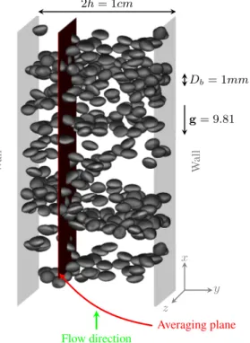
tions. The channel dimensions are 2πh × 2h × πh in x, y and z, where h = 5 mm is the channel half-width (Fig. 1). The flow was computed on a uniform mesh of 85 million hexahedral cells, with 384 × 1152 × 192 cells in x, y and z respectively, hence resolving the flow at the wall up to a first cell-centre of y+ = y/Re
τ = 0.1563. A uniform mesh with a finer
resolu-tion in the wall-normal direcresolu-tion was adopted so as to accurately capture the turbulent structures, while maintaining a satisfactory resolution of the bubbles and their deformations independently of their location in the channel. In this way, we eliminate potential competition between numerical and physical effects in the deter-mination of the wall-normal bubble distribution. Careful atten-tion has been devoted to the consideraatten-tion of physical properties of water and saturated steam similar to PWR conditions for some incidental scenarios where boiling occurs before the depressuri-sation of the system. The physical properties are summarised in Table 1.
Table 1: Physical properties of saturated water and steam (Tsat= 618 K, Psat= 15.5 MPa).
liquid vapour ρ [kg.m-3] 594.38 101.93 µ [Pa.s] 68.327 10−6 23.108 10−6 σ [J.m-2] 4.6695 10−3
The non-dimensional parameters describing the flow are the void fraction α, the ratio of the bubble mean diameter over the channel half-width Db/h, the Reynolds friction, the Atwood, the
Eötvös, the Morton and the Archimedes numbers given by: α = 10%, Db/h = 0.2, Reτ = ρluτh/µl= 180, At = (ρl− ρg)/ρl= 0.83, Eo = (ρl− ρg) gD2b/σ = 1.03, Mo = gµ4l/`ρlσ3´ = 3.53 10−12 and Ar = Eo3/2At−1/2Mo−1/2= ρl(ρl− ρv) gD3b/µ 2 l = 6.15 10 5 . W all W all Flow direction Averaging plane 2h = 1cm Db= 1mm g = 9.81 x y z
Figure 1: Description of the DNS set-up (close-up). x and z are periodic directions.
The computation was initialised with uniformly distributed spherical bubbles. The flow moves upwards along the direction of the gravitational force g = 9.81m.s-2. The motion and defor-mation of 942 bubbles with an equivalent diameter Db = 1mm
is fully resolved by the Front-Tracking algorithm so that the void fraction is αv = 10%. Bubbles leaving the computational
do-main are replicated at the opposite periodic boundary so as to be correctly resolved. The flow-rate is controlled to reach a Reynolds friction number of Reτ = 180. The volumetric flow
rate and the bubble volume are controlled. Thus, after a tran-sitional regime, the flow reaches a statistical steady-state from which statistics can be computed. Converged statistics have been gathered over an averaging period of T = 3.34s of physical time which corresponds to 4 crossing of the channel (of length 2πh), or a non-dimensional period of T+ = T τw/µl = 498 viscous
units. Since the flow variables are spatially homogeneous in x-and z-directions, the statistical average (noted with an overbar ·) is assimilated to the average over time and over the (xz) plane. Every timestep has been used to compute statistics for any cell-centre along the y-axis. Because of flow symmetry, only the aver-ages of the left and right-hand side of the channel are presented. 2.2. Governing equations and numerical method
A finite-difference method with Front-Tracking is used to perform the numerical simulations. In order to avoid spurious current, the “one-fluid” Navier-Stokes equations [3, 14] are for-mulated as follows: ∂ρu ∂t + ∇ · (ρu ⊗ u) = −∇Pn+ ∇ · h µ“∇u + ∇T u”i + Si+ Sf (1) ∇ · u = 0 (2)
Here, u is the velocity vector, ρ and µ are the discontinuous den-sity and viscoden-sity fields respectively (assumed constant for each phase). The source term Sf = Sfxexis introduced in the
stream-wise direction to control the flow rate and to balance, on aver-age, the Archimedean thrust and the wall shear stress. Tempo-ral fluctuations of the source term are controlled by a relaxation equation towards the nominal wall friction τ0= 0.101kg.m-1.s-2
corresponding to a Reynolds number of Reτ = 180. The
aver-aged pressure gradient in the channel generated by gravity and wall friction is modelled by Sfand we resolve a periodic
numer-ical pressure Pnfrom which the averaged pressure gradient due
to wall friction and gravity has been removed. The surface ten-sion term is computed along with the gravitational and possible repellent forces:
Si= (σκ − ∆ρg · xr− φr) ∇χl (3)
Here, g is the gravity vector, σ is the constant surface tension, κ = −∇s· nvis twice the mean curvature (usually negative for
bubbles) and nvis the unit vector normal to the interface,
orien-tated towards the liquid such that nvδi = −∇χlwhere δiis a
three-dimensional delta function located over the interfaces, xr
is the position vector of the real interface1and χlis the phase
in-dicator function equal to 1 in the liquid and 0 in the vapour phase. φris a repellent potential to artificially prevent coalescence and
thereby ensure uniqueness of the bubble’s volume φr= max „ Ir δr− dmin δr , 0 « (4) where dminis the minimal distance towards other bubbles. The
intensity Irof the force and the range δr have been empirically
fitted to their lowest value to prevent coalescence. This force is
1The marker’s position is corrected by L
zero when there is no other inclusion within the range δr.
Be-sides, similar treatment with smaller values was applied at the walls in order to avoid wall contact.
This ad-hoc short-range force has little impact on the local properties of the flow but is necessary to reach a fully-established two-phase turbulent flow. The behaviour of the flow is believed to be more representative of flows with higher Reynolds numbers, not yet achievable via DNS. Suppressing coalescence is a com-mon practice in a classical step-by-step approach to a complex physical problem [6, 17]. The effect of buoyancy forces on the flow dynamics is isolated from other aspects related to liquid film drainage and bubble sliding at a wall. The control of the bub-ble equivalent diameter is also very useful to compare the DNS results to averaged models because we can focus on the mod-elling of turbulence and interfacial forces without perturbation from other models (e. g., for coalescence and break-up) that are rather complicated and influential.
The Navier-Stokes equations are solved by a mixed Volume-Of-Fluid/Front-Tracking (VOF/FT) algorithm similar to Bunner and Tryggvason [3] except for the original discretization of the surface tension and gravitational forces that eliminates spurious current [19]. The original formulation (3) releases the exact mo-mentum conservation in favour of a numerical scheme free of any spurious currents. Mathieu [18] proves that with the new nu-merical formulation, the mechanical energy of the discrete sys-tem decreases when it is isolated, hence allowing an equilibrium state with a zero velocity field. The interface (also called “the Front”) is followed explicitly by connected marker points that are advected by interpolations of the velocity field. Dedicated algo-rithms ensure the preservation of the mesh quality and the volume of each inclusion (based on a VOF-like transport of the phase dicator function). The Front is then used to compute the phase in-dicator function χl, the density and the viscosity on the Eulerian
grid. The algorithm is implemented in the TrioCFD code devel-oped by CEA relying on the TRUST platform (formerly known as Trio_U [4]). The code is fully parallel, written in C++ and has been widely used for industrial applications on single-phase fluid dynamics [e. g., 1, 5, 23].
The algorithm rely on a two-step prediction-correction algo-rithm on a fixed, staggered Cartesian grid, with a third-order ac-curate time advancing scheme [27]. In the prediction step, the source term Siis added to the main flow source term Sf and to
the fourth-order central differentiation of the convection and dif-fusion operators in order to obtain the predicted velocity. Then, an elliptic pressure equation is solved by an algebraic multigrid method to impose a divergence-free velocity field. This part of the algorithm is responsible for most of the computational power consumption (60 to 80% of the whole CPU time), hence spe-cific efforts have been made to improve its efficiency. The new data structure, stored on a Cartesian grid structured by 3 indices (i, j, k) allows heavy strong-scaling with approximately 150 000 elements per processor. Convection and diffusion operators have also been revised to avoid non-contiguous memory access and to improve the use of cache memory.
3. The two fluid model
The DNS presented in section 2 is used as a reference and a source of information for the two-fluid model. In the present work, we focus on adiabatic bubbly flows and micro-to-macroscale model up-scaling is applied to the closure of interfa-cial momentum transfers, setting aside the issue of the Reynolds stresses modelling. Models for interfacial transfers are in fact very influential in two-phase flows and they are chosen as the main interest of the up-scaling methodology presented here. We begin with the definition of averaged and fluctuating quantities. Then, phase-averaging the Navier-Stokes equations and
intro-ducing constitutive relations for the Reynolds stresses and for the interfacial momentum transfers of each phases leads to the two-fluid model [11] solved e. g., in the averaged RANS CFD code NEPTUNE_CFD [10]. The presentation and discussions are mainly focused on the classical hypotheses used to close the interfacial transfers.
3.1. Averaging operator
For practical purpose, the statistical averaging operator [11], noted with an overbar φ, is replaced by the space- and time-averaging using the periodic x and z directions and an time-averaging period ∆t sufficiently large to make φ(y, t) practically indepen-dent of time φ(y, t) ˆ= 1 ∆tLxLz Z t+∆t/2 t−∆t/2 Z Lz 0 Z Lx 0 φ(x, y, z, τ )dxdzdτ Phase or interfacial average are respectively defined by φk k ˆ =χkφk αk and φk i ˆ =φkδ i ai (5) where α = αv = χv is the void fraction and ai = δi is the
interfacial area concentration (IAC). Quantities are then decom-posed into an averaged and a fluctuating part, e. g., for the veloc-ity: uk= ukk+ u
0 k.
3.2. Derivation of the exact equations governing the phase-averaged momentum
The averaged equations describing the evolution of each phase are obtained from the Navier-Stokes equations written for phase k multiplied by the phase indicator function and then aver-aging [7–9, 12, 20]. Due to the commutability of the averaver-aging operator with derivatives, we obtain the following equations ∇ ·“αkukk ” = 0 (6) ∂αkρkukk ∂t + ∇ · “ αkρkukk⊗ u k k ” = −∇αkpkk+ αkρkg + Mk + ∇ ·“αkτkk− αkρku0ku0k k” (7) where τk = µk`∇uk+ ∇Tuk´ is the viscous stress tensor,
Rk= u0ku 0 k
k
the turbulent Reynolds stresses and Mkthe
inter-facial momentum transfers (from the interface to phase k) given by:
Mk= Mi→k= pk∇χk− τk· ∇χk (8)
From the microscopic jump conditions [7, 14], we know that X
k
Mk= Mσ=σκnˆ vδi (9)
where Mσis the mixture momentum source due to surface
ten-sion. Following the proposal of Ishii and Hibiki [12], the macro-scopic interfacial momentum transfer Mkis decomposed using
the surface mean values (noted φik) into
Mk= Mik+ pik∇αk+ ∇αk· τik (10)
where Mik is the total generalised drag force (following Ishii
and Hibiki’s notations [12]). Using Eqns. (9) et (10), one gets the exact macroscopic jump condition at the interface:
Mil+ Miv= Mσ+ “ pil− p i v ” ∇αl+ ∇αl· “ τil− τ i v ” (11) Therefore, this relation states that the imbalance of forces exerted at the interface by both phases is given by the three contributions
on the RHS of Eqn. (11), namely: the mixture momentum source related to surface tension, the interfacial pressure jump and the viscous stress disequilibrium. In the general case, the accumula-tion of energy over the interfaces by means of the surface tension or redistribution between the components of velocity can occur. 3.3. Closures of the phase-averaged momentum
In the context of the two-fluid one-pressure model of dis-persed bubbly flows, it is classically assumed that pik= p
v v= p
l l
and the effect of the interfacial shear τikand the mixture
momen-tum source Mσare often neglected in a first approximation, thus
leading to the approximate macroscopic jump condition at the in-terface:
Mil+ Miv= 0 (12)
In the end, the main variables αv, ull, u v
vand the only pressure2
p describe the evolution of the averaged thermodynamic system. They are governed by four Partial Differential Equations for the vapour, for the total mass and for the liquid and vapour momen-tum conservation, namely
∂αv ∂t + ∇ · (αvu v v) = 0 ∂ (αlρl+ αvρv) ∂t + ∇ · “ αlρlull+ αvρvuvv ” = 0 (13) ∂αlρlull ∂t + ∇ · “ αlρlull⊗ u l l ” = −αl∇p + αlρlg + Mil + ∇ ·“αlτll− αlρlu0lu 0 l l” ∂αvρvuvv ∂t + ∇ · (αvρvu v v⊗ uvv) = −αv∇p + αvρvg + Miv + ∇ ·`αvτvv− αvρvu0vu0v v´ supplemented by constitutive relations to define secondary vari-ables: αl = 1 − αv, u0lu 0 l l , u0 vu0v v , Miland Miv. In
single-phase flow, the closure issue is limited to the modelling of the turbulent Reynolds stresses whereas in two-phase flow, the prob-lem is made more complex by the interactions between phases that produce interfacial momentum transfer.
In the two-fluid Euler-Euler model, the liquid Reynolds stresses Rij = u0lu
0 l l
can be modelled by a second order tur-bulence model (Rij− ε) whereas the vapour Reynolds stresses
are generally neglected: u0 vu0v
v
≈ 0 [10].
As far as the interfacial transfers are concerned, it is very common to use the simplified approximation (12) of Eqn. (11) as a constitutive equation to define e. g., the liquid-to-interface mo-mentum transfer from its vapour counter-part: Mil = −Miv.
Local equilibrium is assumed. One then need to specify the con-tribution on the vapour side (Miv) as a series of forces [12, 20].
For instance in NEPTUNE_CFD [10], the model of Ishii and Zu-ber [13] is used to model the drag force. The virtual mass and Basset forces are accounted for by means of Zuber’s model [28]. The lift and wall lubrication forces are presented in Tomiyama [21] and Tomiyama et al. [22]. Lastly, the model for turbulent dis-persion force is given in Laviéville et al. [16]. For completeness, one should stress that those models require additional informa-tion on the flow topology, such as the distribuinforma-tion of the bubble diameters for instance. A modelled equation governing the in-terfacial area transport is therefore usually necessary but this is beyond the scope of this paper. Finally, the set of equations (13) can be solved in averaged codes to predict the flow evolution.
In the next section, the DNS data is used to assess the assump-tion of interfacial momentum equilibrium given by Eqn. (12).
4. Results and discussion
This section starts with wall-normal profiles of mean vari-ables and the comparison of macroscopic flow characteristics to the equivalent single-phase flow. Then, in the up-scaling method-ology, information on the macroscopic jump condition at the in-terface is extracted from the DNS results. The procedure used to compute several contributions is presented. Each term of Eqn. (11) is evaluated as a function of the distance to the wall and the validity of the assumption of interfacial momentum equi-librium (Eqn. (12)) is therefore assessed.
4.1. Mean variables
As a consequence of the high void fraction considered and of the preservation of a realistic buoyancy force, the flow exhibits a behaviour that, to our knowledge, has not been observed yet. Nei-ther wall nor core peaking of the void fraction appears (Fig. 2). The repellent forces used to prevent wall contact are only effec-tive up to y+ ≈ 5.8 and the void fraction is nil for y+< 2. The
void fraction profile at steady-state results from the intricate bal-ance between the turbulent shear, the surface tension force and the Archimedean thrust. The bubble distribution remains rather homogeneous with α ≈ 10.3%, even in the wall normal direc-tion. Close to the wall, two consecutive peaks are observed at y+≈ 27 and y+≈ 68. Figure 2 shows that the peaks fit well to
the law that would be obtained for a layer of spherical bubbles α(y+) = αmax 1 − `y+− y c ´2 r2 a ! (14) where αmax is the maximum void fraction, yc = ra+ δ is
the location of this peak defined by the apparent bubble ra-dius raand the offset between the wall and the bubble layer δ.
The triplet (αmax, ra, δ) for each peak is: (13.4%, 25, 2) and
(10.9%, 50, 18). The equivalent dimensionless radius of the bub-bles is r+b = 18. From visual inspection of Fig. 1, bubbles are slightly elongated in the wall-normal direction. A meandering pattern of the bubbles is added to these deformations to result in the void fraction profile of Fig. 2. Hence, in the near-wall layer, the lateral motion of bubbles is rather limited whereas in the sec-ond layer their trajectories are more scattered in the wall-normal direction. In actual fact, bubbles are not trapped in any layer.
Figure 3 shows the liquid, the vapour and the mixture velocity profiles. The relative velocity between the liquid and the bubbles is very strong. The signature of the first void fraction peak is clearly visible. In the viscous and buffer layers (y+ < 20), the liquid velocity follows the power law u+ = 1.211`y+´0.6215
and the mixture velocity is similar to the liquid velocity in a single-phase flow for the same pressure drop. However, after the void fraction wall peaks, the velocity gradient is smaller than for a pure liquid flow, hence leading to the following log law: u+= 1/k ln`y+´ + B
with: k = 1.3 and B = 5.2 (15) The values of k and B in a low-Reynolds single-phase turbulent flow are: k = 0.4 and B = 5.5 [15].
4.2. Assessment of the macroscopic jump relation
In order to evaluate the terms of Eqn. (11), one needs to post-process the DNS results so as to estimate Mk, pikand τ
i k. Such
interfacial quantities are very difficult to compute directly be-cause some local instantaneous one-fluid fields (such as µ, p, ∇u) are discontinuous at the interface. Consequently, any attempt to evaluate Mk directly from its definition (8) or pikand τ
i kfrom
their local discretized values at the interface is subjected to con-siderable uncertainty and is likely to be useless for the analysis of the balance (11). Therefore, we have preferred to evaluate Mkby
Figure 2: Void fraction profile. Figure 3: Velocities profiles.
computing the other terms in the averaged momentum equation (Eqn. (7)). Besides, interfacial averaged quantities are assumed equal to the phase-average following a similar reasoning as for the closure of the two-fluid model [12]: pik≈ p
k k and τ i k≈ τ k k.
Then, Mikcan be constructed from Eqn. (10). Furthermore, the
interfacial mixture momentum Mσis readily accessible with our
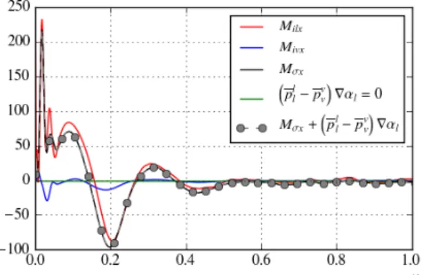
numerical method as it is the average of a part of Siin Eqn. (3). Following this procedure, the terms of Eqn. (11) are com-puted and plotted in Figs. 4 and 5 for streamwise and wall-normal components respectively. The viscous stresses τkk have been
found negligible and are not presented for simplicity. The repel-lent forces used to preserve the topology of the flow (monodis-persed bubbles) act randomly on the bubbles and their intensity is sufficiently small to result in a negligible contribution behind the surface tension term Mσ.
In the streamwise direction, there is no gradient of void frac-tion because the flow is periodic. Therefore, Eqn. (11) simply reduces to:
Milx+ Mivx= Mσx (16)
Figure 4 shows that the vapour contribution Mivxis roughly
nil through the channel whereas the liquid part Milxis almost
equal to the surface tension source term Mσx. Therefore, Mσx
cannot be neglected and is fully responsible for the momentum source term acting on the liquid axial momentum.
Besides, we recall that the bubble mean diameter is Db/h = 0.2 and that the contribution of surface tension is nil
over closed portions of interfaces. Therefore, we can infer from Fig. 4 that energy is taken from the liquid in the near-wall layer. It is stored onto the interfaces via their deformations and takes the form of surface tension energy of the mixture. Then, when waves propagates along the interface or when bubbles moves away from the wall, this energy may be released and dissipated into the liq-uid. A similar process seems to take place around the secondary peak of the void fraction.
The two strong spikes for y/h < 0.05 may not be physi-cal and could be related to imprecision in the a posteriori dif-ferentiation operators used to evaluate Mkor in the poor
resolu-tion of small interfacial structures. In the centre of the channel (y/h > 0.5), both phases are in equilibrium and almost no mo-mentum transfer takes place (apart from buoyancy effect).
Figure 5 shows the budget of wall-normal components. Con-tributions are much larger than in the spanwise direction. Alter-nate positive and negative values also characterise intense trans-fers at the scale of the bubble diameter. In first approximation, Milyand Mivyare balancing each other out but the surface
ten-sion and the pressure difference still represents around 10% of Milyeach.
Finally, this work reveals that in the conditions of this DNS (high void fraction and pressurised steam/water), the single pres-sure and negligible surface tension hypotheses are not accurate: Mivx≈ 0, Mσx≈ Milx, Mivy≈ −0.8Mily,
“ pll− p
v v
”∂αl
∂y ≈ 0.1Mily and Mσy≈ 0.12Mily (17) Thus, new models for the pressure difference and for interfacial energy should be investigated. For instance, the derivation of a transport equation for the interfacial energy related to surface tension could be investigated based on physical principles and on the microscopic jump conditions. In a second step, constitutive relations for the sink and source terms in this equation will be necessary and will require additional modelling efforts.
5. Conclusion
The DNS of a bubbly flow in a channel in conditions close to reactor core was achieved for a Reynolds friction number Reτ= 180 and a void fraction α = 10%. At statistically
steady-state, the void fraction profile results of the complex equilibrium
Figure 4: Streamwise contributions to the averaged macro-scopic jump condition evaluated from DNS results.
Figure 5: Wall-normal contributions to the averaged macro-scopic jump condition evaluated from DNS results.
between buoyancy, surface tension and shear stresses. Some vari-ations of the void fraction and the velocity profiles are clearly re-lated to the characteristic bubble size. Two small void fraction peaks are observed near the wall whereas the two phases reach an equilibrium in the centre of the channel with no momentum transfer and a uniform void fraction. Velocity profiles are also analysed. The flow-rate reduction in two-phase flow is related to the effect of the void fraction main peak and to a strong reduction of the velocity gradient in the log law region.
Then, the DNS data is used as a reference to compare to the single-pressure one-fluid model of NEPTUNE_CFD. Upscaling process towards two-phase RANS CFD modelling is covered fo-cusing on momentum interfacial transfers. In the streamwise di-rection, the force exerted by the liquid is stored over the interfaces as interfacial energy due to surface tension. In the wall-normal direction, inter-phases transfers are much stronger and more ef-ficient. Pressure difference and surface tension force only rep-resent 10% of this transfer each. Hence, some very common hypotheses of two-fluid models such as the negligible effect of surface tension on mean flow properties or the single pressure are challenged and our work suggests they should be revised. Future modelling efforts should focus on the interfacial transfer closure for instance looking for the derivation and the closure of a trans-port equation for the interfacial surface tension energy.
References
[1] Aulery, F., Toutant, A., Bataille, F., and Zhou, Y. En-ergy transfer process of anisothermal wall-bounded flows. Physics Letters A, 379(24 – 25):1520 – 1526, 2015. [2] Bois, G. Direct Numerical Simulation of a turbulent bubbly
flow in a vertical channel: Towards an improved Second-Order Reynolds Stress Model. Nuclear Engineering and Design, 2016. Submitted.
[3] Bunner, B. and Tryggvason, G. Effect of bubble deforma-tion on the properties of bubbly flows. Journal of Fluid Mechanics, null:77–118, 2003.
[4] Calvin, C., Cueto, O., and Emonot, P. An object-oriented approach to the design of fluid mechanics software. ESAIM: M2AN, 36(5):907–921, 2002. <http://www-trio-u.cea.fr>. [5] Chandesris, M., D’Hueppe, A., Mathieu, B., Jamet, D., and
Goyeau, B. Direct numerical simulation of turbulent heat transfer in a fluid-porous domain. Physics of Fluids, 25(12), 2013.
[6] Dabiri, S. and Tryggvason, G. Heat transfer in turbulent bubbly flow in vertical channels. Chemical Engineering Sci-ence, 122(0):106 – 113, 2015.
[7] Delhaye, J.-M. Jump conditions and entropy sources in two-phase systems. Local instant formulation. International Journal of Multiphase Flow, 1:395–409, 1974.
[8] Delhaye, J.-M. Thermohydraulique des réacteurs. EDP Sciences, 2008.
[9] Drew, D. A. and Passman, S. L. Theory of Multicomponent Fluids. Springer Verlag, New York, 1999.
[10] Guingo, M., , and Equipe de Développement NEP-TUNE_CFD. NEPTUNE_CFD 3.0.0 Theory Guide. Tech-nical report, EDF, 2015.
[11] Ishii, M. Thermo-Fluid Dynamic Theory of Two-phase Flow. Collection de la Direction des études et recherches d’Électricité de France. Eyrolles, 1975.
[12] Ishii, M. and Hibiki, T. Thermo-Fluid Dynamics of Two-Phase Flow. SpringerLink : Bücher. Springer New York, 2010.
[13] Ishii, M. and Zuber, N. Drag coefficient and relative veloc-ity in bubbly, droplet or particulate flows. AIChE Journal, 25(5):843–855, 1979.
[14] Kataoka, I. Local instant formulation of two-phase flow. International Journal of Multiphase Flow, 12(5):745–758, 1986.
[15] Kim, J., Moin, P., and Moser, R. Turbulence statistics in fully developed channel flow at low reynolds number. Jour-nal of Fluid Mechanics, 1987.
[16] Laviéville, J., Mérigoux, N., Guingo, M., Baudry, C., and Mimouni, S. A Generalized Turbulent Dispersion Model for bubbly flow numerical simulation in NEPTUNE_CFD. In Proceedings of the 16th NURETH conference, Kanazawa, Japan, 2015.
[17] Lu, J. and Tryggvason, G. Effect of bubble deformability in turbulent bubbly upflow in a vertical channel. Physics of Fluids, 20(4):040701, 2008.
[18] Mathieu, B. Études physique, expérimentale et numérique des mécanismes de base intervenant dans les écoulements diphasiques en micro-fluidique. PhD thesis, Université de Provence, 2003.
[19] Mathieu, B. A 3D parallel implementation of the Front-Tracking method for two-phase flows and moving bod-ies. In 177ème Session du comité scientifique et technique de la Société Hydrotechnique de France, Advances in the modelling methodologies of two-phase flows, Lyon, France, November 24-26, 2004. Paper # 24.
[20] Morel, C. Mathematical Modeling of Disperse Two-Phase Flows. Springer International Publishing, 2015.
[21] Tomiyama, A. Struggle with computational fluid dynam-ics. In Third International Conference on Multiphase Flow. ICMF 98, Lyon, France, 1998.
[22] Tomiyama, A., Tamai, H., Zun, I., and Hosokawa, S. Trans-verse migration of single bubbles in simple shear flows. Chemical Engineering Science, 57(11):1849–1858, 2002. [23] Toutant, A. and Bataille, F. Turbulence statistics in a fully
developed channel flow submitted to a high temperature gradient. International Journal of Thermal Sciences, 74(0): 104 – 118, 2013.
[24] Tryggvason, G. and Lu, J. Direct Numerical Simulations of flows with phase change. Procedia IUTAM, 15:2 – 13, 2015. IUTAM Symposium on Multiphase Flows with Phase Change: Challenges and Opportunities.
[25] Tryggvason, G., Esmaeeli, A., Lu, J., and Biswas, S. Di-rect Numerical Simulations of gas/liquid multiphase flows. Fluid Dynamics Research, 38(9):660 – 681, 2006. Recent Topics in Computational Fluid Dynamics.
[26] Tryggvason, G., Dabiri, S., Aboulhasanzadeh, B., and Lu, J. Multiscale considerations in Direct Numerical Simulations of multiphase flows. Physics of Fluids, 25(3):031302, 2013. [27] Williamson, J. Low-storage Runge-Kutta schemes. Journal
of Computational Physics, 35(1):48 – 56, 1980.
[28] Zuber, N. On the dispersed two-phase flow in the laminar flow regime. Chemical Engineering Science, 19:897, 1964.