HAL Id: pastel-00912565
https://pastel.archives-ouvertes.fr/pastel-00912565
Submitted on 2 Dec 2013HAL is a multi-disciplinary open access archive for the deposit and dissemination of sci-entific research documents, whether they are pub-lished or not. The documents may come from teaching and research institutions in France or abroad, or from public or private research centers.
L’archive ouverte pluridisciplinaire HAL, est destinée au dépôt et à la diffusion de documents scientifiques de niveau recherche, publiés ou non, émanant des établissements d’enseignement et de recherche français ou étrangers, des laboratoires publics ou privés.
basins : A hydrological modelling approach
Raji Pushpalatha
To cite this version:
Raji Pushpalatha. Low-flow simulation and forecasting on French river basins : A hydrological mod-elling approach. Earth Sciences. AgroParisTech, 2013. English. �NNT : 2013AGPT0012�. �pastel-00912565�
Doctorat ParisTech
École doctorale Géosciences et Ressources naturelles
THÈSE
pour obtenir le grade de docteur délivré par
L’Institut des Sciences et Industries
du Vivant et de l’Environnement
(AgroParisTech)
Spécialité: Hydrologie
Raji PUSHPALATHA
18 janvier 2013
Low-flow simulation and forecasting on
French river basins: a hydrological modelling approach
Simulation et prévision des étiages sur des bassins versants français : approche fondée sur la modélisation hydrologique
Directeur de thèse : Vazken ANDRÉASSIAN Co-encadrement de la thèse : Charles PERRIN
Jury
Mme Florentina MOATAR Université François Rabelais, Tours Rapporteur
M. Christophe BOUVIER UMR Hydrosciences, Montpellier Rapporteur
M. Laurent PFISTER Institut Gabriel Lippmann, Belvaux Examinateur
M. Thibault MATHEVET EDF-DTG, Grenoble Examinateur
M. Pascal MAUGIS ONEMA, Vincennes Invité
AgroParisTech
Irstea, Unité de recherche Hydrosystèmes et Bioprocédés 1 rue Pierre-Gilles de Gennes, CS 10030, 92761 Antony cedex
Acknowledgements
I would like to thank several people and organizations for their invaluable helps to fulfil this work. First of all I would like to express my heartfelt thanks to my supervisor Dr. Charles Perrin, Irstea, Antony, France, for his valuable guidance, critical suggestions and immense help throughout my PhD. I have immense pleasure to express my sincere gratitude to Dr. Vazken Andréassian, head of the hydrology group, Irstea, for his support, suggestions and constant encouragements during the course of the project. I am also indebted to Dr. Maria-Helena Ramos, Irstea, for her valid advices at different phases of my work. I am expressing my sincere gratitude to Dr. Cécile Loumagne and Didier Pont, respectively former and current head of the HBAN unit, Irstea, for their support. I wish also to thank Pr. Florentina Moatar, Dr. Christophe Bouvier, Dr. Laurent Pfister, Dr. Thibault Mathevet and Dr. Pascal Maugis, for accepting to be part of the jury and to evaluate this work.
I am thankful to Peschard Julien who was always ready to make series of maps throughout my work. I acknowledge Dr. Nicolas Le Moine and Dr. Thibault Mathevet for their valuable suggestions at different phases of my work.
I am very grateful to Météo-France for providing meteorological data and SCHAPI for providing flow data necessary to carry out my tests. The last chapter of this thesis could not have been carried out without the help of Thibault Mathevet (EDF-DTG) and Claudine Jost (Seine Grands Lacs) who helped building the database and who are thanked for that. I also wish to thank DIM ASTREA of Région Ile-de-France, as well as ONEMA, for their financial support to conduct this study.
I express my sincere gratitude to Dr. Elisabeth Maltese for the interesting French classes and her guidance.
I express my gratitude to Dr. Lionel Berthet, Dr. Audrey Valery, Marine Riffard and Dr. Mamoutou Tangara for their help and support throughout my work.
I acknowledge my gratitude to my colleagues: Ioanna, Annie, François, Florent, Laurent, Gianluca, Pierre, Pierre-Yves and Damien for their help and support throughout my work period at Irstea.
I am also extremely thankful to my friends: Dr. Agnel Praveen Joseph, Dr. Sunil Kumar, Rubie M Sam, Dr. Sonam Popli, Dr. Debjani Bagchi, Dr. Prasanth Karikkethu and Ananya at Cité Universitaire for their support throughout my stay in Paris.
I am most grateful to my parents and my sister for the love and affection they showered on me and the support they have shown during this long yet rewarding process of finishing my degree.
The words fail me to express my appreciation to one, whose love and persistent confidence in me, has taken the load off my shoulder. I owe Dr. Govindan Kutty, my husband, for being unselfishly let his intelligence, passions, and ambitions collide with mine.
Abstract
Long-term stream low-flow forecasting is one of the emerging issues in hydrology due to the escalating demand of water in dry periods. Reliable long-lead (a few weeks to months in advance) streamflow forecasts can improve the management of water resources and thereby the economy of the society and the conditions for aquatic life. The limited studies on low flows in the literature guided us to address some of the existing issues in low-flow hydrology, mainly on low-flow simulation and forecasting. Our ultimate aim to develop an ensemble approach for long-term low-flow forecasting includes several prior steps such as characterisation of low flows, evaluation of some of the existing model’s simulation efficiency measures, development of a better model version for low-flow simulation, and finally the integration of an ensemble forecasting approach.
A set of catchments distributed over France with various hydrometeorological conditions are used for model evaluation. This data set was first analysed and low flows were characterized using various indices. Our objective to better evaluate the models’ low-flow simulation models resulted in the proposition of a criterion based on the Nash-Sutcliffe criterion, but calculated on inverse flows to put more weight on the errors on extreme low flows. The results show that this criterion is better suited to evaluate low-flow simulations than other commonly used criteria.
Then a structural sensitivity analysis was carried out to develop an improved model structure to simulate stream low flows. Some widely used models were selected here as base models to initiate the sensitivity analysis. The developed model, GR6J, reaches better performance in both low- as well as high-flow conditions compared to the other tested existing models. Due to the complexity of rainfall-runoff processes and the uncertainty linked to future meteorological conditions, we developed an ensemble modelling approach to issue forecasts and quantify their associated uncertainty. Thus the ensemble approach provides a range of future flow values over the forecasting window. Here observed (climatological) rainfall and temperature were used as meteorological scenarios fed the model to issue the forecasts. To reduce the level of uncertainty linked to the hydrological model, various combinations of simple updating procedures and output corrections were tested. A straightforward approach, similar to what can be done for flood forecasting, was selected as it proved the most efficient.
Last, attempts were made to improve the forecast quality on catchments influenced by dams, by accounting for the storage variations in upstream dams. Tested on the Seine and Loire basins, the approach showed mixed results, indicating the need for further investigations.
Résumé
La prévision d’étiage à long terme est l'une des questions émergentes en hydrologie en raison de la demande croissante en eau en période sèche. Des prévisions fiables de débits à longue échéance (quelques semaines à quelques mois à l'avance) peuvent améliorer la gestion des ressources en eau et de ce fait l'économie de la société et les conditions de vie aquatique. Les études limitées sur les étiages dans la littérature nous a conduit à traiter certaines des questions existantes sur l’hydrologie des étiages, principalement sur la simulation et la prévision des étiages. Notre objectif final de développer une approche d'ensemble pour la prévision à long terme des étiages se décline en plusieurs étapes préalables, telles que la caractérisation des étiages, l'évaluation de mesures existantes d'efficacité des simulations des modèles, le développement d'une version améliorée d’un modèle de simulation des étiages, et enfin l'intégration d’une approche de prévision d'ensemble.
Un ensemble de bassins distribués partout en France avec une variété de conditions hydro-météorologiques a été utilisé pour l’évaluation des modèles. Cet échantillon de données a d’abord été analysé et les étiages ont été caractérisés en utilisant divers indices. Notre objectif de mieux évaluer les simulations des étiages par les modèles a conduit à proposer un critère basé sur le critère de Nash-Sutcliffe, calculé sur l’inverse des débits pour mettre davantage de poids sur les erreurs sur les très faibles débits. Les résultats montrent que ce critère est mieux adapté à l’évaluation des simulations des étiages que d’autres critères couramment utilisés.. Une analyse de sensibilité structurelle a ensuite été menée pour développer une structure de modèle améliorée pour simuler les étiages. Des modèles couramment utilisés ont été choisis ici comme modèles de base pour commencer l'analyse de sensibilité. Le modèle développé, GR6J, atteint de meilleures performances à la fois sur les faibles et les hauts débits par rapport aux autres modèles existants testés.
En raison de la complexité du processus pluie-débit et de l'incertitude liée aux conditions météorologiques futures, nous avons développé une approche d'ensemble pour émettre des prévisions et quantifier les incertitudes associées. Ainsi l'approche d'ensemble fournit une gamme de valeurs futures de débits sur la plage de prévision. Ici, la climatologie a été utilisée pour fournir les scénarios météorologiques en entrée du modèle pour réaliser les prévisions. Pour réduire le niveau d’incertitude lié au modèle hydrologique, des combinaisons variées de procédures de mise à jour et de corrections de sortie ont été testées. Une approche directe,
similaire à ce qui peut être fait pour la prévision des crues, a été sélectionnée comme la plus efficace.
Enfin, des essais ont été réalisés pour améliorer la qualité des prévisions sur les bassins influencés par les barrages, en tenant compte des variations de stockage dans les barrages amont. Testée sur les bassins de la Seine et de la Loire, l’approche a donné des résultats mitigés, indiquant le besoin d’analyses complémentaires.
Table of contents
Acknowledgements ... 1
Abstract ... 3
Résumé ... 5
Table of contents ... 7
List of Tables ... 11
List of Figures ... 12
General introduction ... 1
Introduction ... 3Evaluation of model's low-flow simulation efficiency ... 4
Why a general model structure for the French river basins? ... 4
Long-term forecasting of low flows and possible improvements ... 5
Exploratory tests to make low-flow forecasts on catchments influenced by dams ... 5
Organisation of thesis ... 6
Part I: Stream low flows and their characterization ... 7
Chapter 1. Low flows and low-flow generating factors in the French context ... 11
1.1. Introduction ... 13
1.2. Natural influences on low flows: catchment characteristics ... 15
1.2.1. Catchment geology and river low flows ... 16
1.3. Anthropogenic impacts on catchment characteristics and low flows ... 18
1.3.1. Direct influences ... 18
1.3.2. Indirect influences ... 19
1.4. Potential impacts of climate change on future river flows ... 20
1.5. Impact of low flows on society ... 21
1.6. Conclusions ... 21
Chapter 2. Data set and low-flow characterisation ... 23
2.1. Introduction ... 25
2.2. Description of the catchment set ... 25
2.2.1. Catchment selection ... 25
2.2.1. Data sets ... 27
2.2.2. Sample catchments ... 28
2.3. Low-flow measures ... 30
2.3.1. Low-flow period (low-flow spells) ... 31
2.3.2. Flow duration curve (FDC) ... 31
2.3.4. Base-flow index (BFI) ... 31
2.4. Computations of low-flow indices on the study catchment set ... 32
2.5. Link between low-flow indices ... 36
2.6. Low-flow indices and catchment descriptors ... 38
2.6.1. Aridity index (AI) ... 38
2.6.2. Catchment geology ... 39
2.7. Conclusions ... 40
Part II: Stream low-flow simulation ... 43
Chapter 3. Analysis of efficiency criteria suitable for low-flow simulation ... 47
3.1. Introduction ... 49
3.2. Criteria used for the evaluation of low–flow simulation... 50
3.2.1. Are existing criteria appropriate to evaluate low-flow simulations? ... 53
3.3. Scope of the study ... 54
3.4. Models and evaluation methodology ... 55
3.4.1. Hydrological models ... 55
3.4.2. Testing scheme ... 58
3.4.3. Criteria analysed ... 58
3.4.4. Approach for criterion analysis ... 61
3.5. Results and discussion ... 64
3.5.1. Overall efficiency distribution ... 64
3.5.2. Criteria interdependency ... 65
3.5.3. Analysis of model error terms ... 68
3.5.4. Which criterion should be used for low–flow evaluation?... 69
3.5.5. What should be done with zero flows when calculating * iQ NSE ? ... 70
3.5.6. Power transformation and criteria ... 71
3.6. Conclusions ... 73
Chapter 4. Development of an improved lumped model for low-flow simulation 75
4.1. Introduction ... 774.2. Selection of basic model structures ... 77
4.3. Model testing ... 78
4.4. Evaluation of the selected model structures ... 79
4.5. Development of an improved model structure from the base models ... 80
4.5.1. Integration of groundwater exchange function (F) ... 81
4.5.2. Addition of new stores ... 84
4.6. Results and discussion ... 86
4.6.1. Can the existing groundwater exchange term in GR5J be improved? ... 86
4.6.2. Should the volumetric splitting between flow components be adapted to each catchment? ... 87
4.6.3. Should a new store be added in series or in parallel? ... 88
4.6.4. Does the formulation of routing stores matter? ... 89
4.6.5. Comparing the results of GR5J and GR6J ... 90
4.6.6. Illustration of model's results ... 91
4.1. Conclusions ... 95
Part III: Stream low-flow forecasting ... 97
Chapter 5. Low-flow forecasting: implementation and diagnosis of a long-term
ensemble forecasting approach ... 101
5.1. Introduction ... 103
5.2. Literature on long-term forecasting in the French River basins ... 104
5.3. Scope of the study ... 105
5.4. Methodology ... 105
5.4.1. An ensemble approach towards low-flow forecasting ... 106
5.4.2. Description of the forecasting approach ... 107
5.5. How to improve the quality of a model forecast? ... 108
5.5.1. Output bias corrections ... 110
5.5.2. Model updating to improve the forecast quality ... 111
5.6. Assessment of the forecasting system ... 113
5.6.1. Measure based on error in magnitude ... 113
5.6.2. Measures based on contingency table ... 114
5.6.3. Measure based on probability ... 115
5.7. Results and discussion ... 117
5.7.1. How long are model forecasts useful (without any corrections)? ... 118
5.7.2. Influence of simulation error on model forecasts ... 119
5.7.3. How to improve model’s forecast quality? ... 120
5.7.1. Maximum possible lead-time (MPLT) ... 128
5.8. Conclusions ... 135
Chapter 6. Accounting for the influence of artificial reservoirs in low-flow
forecasting ... 137
6.1. Introduction ... 139
6.2. Scope of the study ... 140
6.3. Test catchments ... 140
6.1. Methodology ... 142
6.1.1. To account for the reservoirs into an R-R model ... 142
6.1.2. Model testing and evaluation ... 145
6.2. Results and discussion ... 145
6.2.1. Can we really improve the simulation performance of models by accounting the reservoirs? ... 145
6.2.2. Can we improve the forecast quality? ... 148
6.3. Conclusion ... 150
General conclusion ... 151
Synthesis ... 153
Perspectives ... 154
Appendices ... 173
A Selection of objective function for calibration ... 175
A.1 Test of a set of criteria ... 177
B A review of efficiency criteria suitable for evaluating low-flow simulations ... 179
C Description of the hydrological models tested in this study ... 193
C.1 Model Gardénia (GARD) ... 197
C.2 GR-series (GR4J & GR5J) ... 198 C.3 HBV0 ... 200 C.4 IHAC ... 201 C.5 MOHY ... 202 C.6 MORD ... 203 C.7 TOPM ... 204
D The developed model versions and their performances ... 205
D.1 Versions of model GR4J ... 207
D.2 Test results of versions of GR4J ... 208
D.3 Performance of versions of MORD & TOPM ... 208
E A downward structural sensitivity analysis of Hydrological models to improve low-flow simulation ... 211
F Model's sensitivity to temporal variations of potential evapotranspiration .... 225
F.1 Introduction ... 227
F.2 Tested models ... 228
F.3 Results and discussion ... 229
List of Tables
Table 2.1 Variability in size and the main hydroclimatic conditions over the catchment set ... 27
Table 2.2: Characteristics of sample catchments... 29
Table 3.1: Studies that used criteria to evaluate low-flow simulation quality... 51
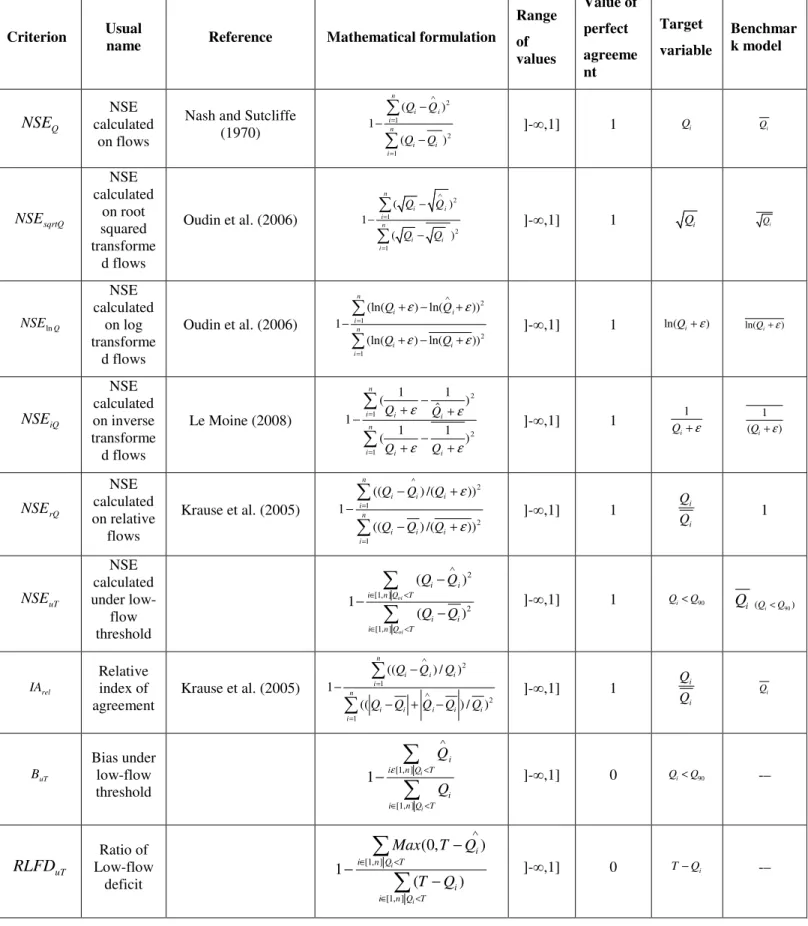
Table 3.2: Selection of evaluation criteria and their corresponding formulation and specific values (Qiand Qi ∧ are the observed and simulated flows, respectively, n the total number of time steps, Ta low-flow threshold (here T =Q90), Q the mean of Q, and ε a small constant) ... 60
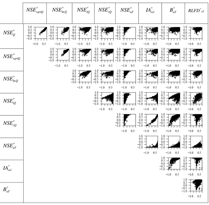
Table 3.3: Scatter plots of pairs of criteria on the 940–catchment set for the GR4J in validation ... 66
Table 3.4: The Spearman correlation coefficient for the criteria corresponding to the plots in Table 3.3 ... 66
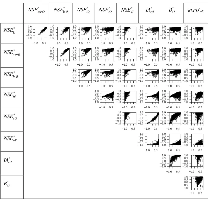
Table 3.5: Scatter plots of pairs of criteria on the 940–catchment set for the MORD in validation ... 67
Table 3.6: The Spearman correlation coefficient for the criteria corresponding to the plots in Table 3.5 ... 67
Table 4.1: Selected model structures and their number of parameters ... 78
Table 4.2: Average efficiency values in validation for the lumped models for various criteria (criteria on Q and iQ put more emphasis on high flows and low flows, respectively, and criterion on lnQ is intermediate). ... 79
Table 4.3: Modified versions of the GR5J model in terms of groundwater exchange function ... 83
Table 4.4: Modified versions of the GR5J model and their main characteristics ... 85
Table 4.5: Mean model performance for versions M4 and M5 ... 87
Table 4.6: Mean efficiency values for versions M5 and M6 ... 88
Table 4.7: Mean model performance for versions M8–M11 (multiple routing stores) and mean relative performance RE* with reference to M8 over the catchment set ... 88
Table 4.8: Mean efficiency values of M8 vs M12 ... 90
Table 4.9: Mean performance of GR5J and GR6J and relative performance of GR6J with reference to GR5J over the catchment set for various criteria (criteria on Q and iQ put more emphasis on floods and low flows, respectively). The results were obtained in validation ... 91
Table 5.1: Notations and their definitions (Q- observed streamflow; Qˆ - simulated flow; Qˆf - forecast value; Qˆˆf - corrected forecast value) ... 109
Table 5.2: Formulations of bias corrections and model updating techniques used in this study... 110
Table 5.3: Formulations of model output updating techniques ... 112
Table 5.4: Contingency table ... 114
Table 5.5: Scores based on the contingency table ... 114
Table 5.6 Median values of the BSS for the different correction procedures ... 129
Table 6.1: Summary of data set in the Seine basin ... 143
List of Figures
Figure 1.1: Natural hydrological processes and catchment storages (WMO, 2008) ... 13
Figure 1.2: Illustration of stream low flows of one of the study catchments (Catchment L’Aber Wrac’h at Le Drennec) for a period of three years (2003-2005) ... 14
Figure 1.3: Left: Summer low flows of the Garonne River downstream Toulouse (Source: A. Dutartre, Irstea) and right: winter low flows of the Columbia River, Canada (Source: WMO, 2008) .... 15
Figure 1.4 Geological map of France (Source: Geological Survey of France) ... 17
Figure 1.5 Total water availability and its utility by different sectors in France in 2009 (Source: Commissariat général au développement durable, 2012) ... 19
Figure 1.6: Changes in the annual discharges (using SIM model) between the 2046-2065 and 1971-2000 periods averaged over France using the inputs from 14 climate models (Source: Boé et al., 2009) ... 20
Figure 2.1: Location of 1000 catchments of the data set (the highlighted background indicates the presence of mountains) ... 26
Figure 2.2: Mean Q/P vs P/PE values for the catchments in the data set ... 28
Figure 2.3: Illustration of location of sample catchments and their daily flow hydrographs from 2003 to 2005 ... 30
Figure 2.4: Illustration of the period of occurrence of low-flows in the test data set ... 33
Figure 2.5: Flow duration curve of the sample catchments for a period of 2003 to 2005 (the values below 0.1 mm/d are not shown) ... 34
Figure 2.6: Illustration of spatial variability of the low-flow indices: (a) - MAM7; (b) - QMNA5; (c) - Q90/Q50; (d) - BFI ... 36
Figure 2.7: Relation between Q90 and MAM7 ... 37
Figure 2.8: Relation between QMNA5 and MAM7 ... 37
Figure 2.9: Aridity index vs. low-flow indices ... 38
Figure 2.10: Boxplots of distribution of Q90 values of catchments based on their geology (boxes represent the 0.25 and 0.75 percentiles, with the median value inside, and the whiskers represent the 0.10 and 0.90 percentiles) ... 39
Figure 2.11: Distribution of BFI values based on geology (boxes represent the 0.25 and 0.75 percentiles, with the median value inside, and the whiskers represent the 0.10 and 0.90 percentiles) ... 40
Figure 3.1: Illustration of changes in the series of flows, model errors and cumulated squared errors using root square and logarithm transformations for the Moselle River at Custines (Hydro code: A7010610; catchment area: 6830 km²; period: 01/01/1980–31/12/1981). ... 54
Figure 3.2 Schematic diagrams of the structures of (a) the GR4J model and (b) the MORD model (PE: potential evapotranspiration; P: rainfall; Q: streamflow; X parameters; other letters are internal model variables) ... 56
Figure 3.3: Box plots of performance (NSE* Q in validation) of the GR4J model on the 940 catchments as a function of catchment size (boxplots show the 0.05, 0.25, 0.5, 0.75 and 0.95 percentiles from bottom to top; each box plot contains one tenth of catchments) ... 57
Figure 3.4: Example of derivation of box plots from the distribution of weighted flows (here weights are the squared errors) to the flow duration curve (distribution of non weighted flows). The same example as in Figure 3.1 is used here (Period: 01/01/1980 – 3112/1981) ... 62 Figure 3.5: Illustration of flow values that contribute the most of the total model error. The error considered here is the square error calculated on flows. The darker the dots, the larger the contribution to the total error. Horizontal dashed lines correspond to the percentiles of the box plot shown in Figure 3.4. ... 63 Figure 3.6: Schematic representation of the derivation of master box plot which summarizes the behaviour of a given criterion over the entire catchment set (M stands for the total number of catchments) ... 63 Figure 3.7: Box plot of distribution of efficiency criteria obtained by the GR4J and MORD models over the entire catchment set in validation (boxes represent the 0.25 and 0.75 percentiles, with the median value inside, and the whiskers represent the 0.05 and 0.95 percentiles) ... 64 Figure 3.8: Master box plot obtained over the entire catchment set for the GR4J and MORD models (each flow percentile of exceedance corresponds to the median of this percentile over all the box plots obtained on each catchment of the entire set) ... 68 Figure 3.9: Change in the mean value of NSEiQ* and NSEln Q* obtained by the GR4J model in validation over the catchment set with different values of ε (fractions of Qm from Qm/10 to Qm/100) ... 70 Figure 3.10: Comparison of values obtained by GR4J (left) and MORD (right) models for the two test periods (P1 and P2) ... 72 Figure 3.11: Comparison of λ values obtained by the GR4J and MORD models ... 72 Figure 3.12: Scatter plot of Q90/Q50 vs. lambda values ( ) for the two test periods for the GR4J model
... 73 Figure 4.1: Structural layout of the base models ... 80 Figure 4.2: Layout of two versions of the GR5J model with different additional stores ... 85 Figure 4.3: Box plots of NSE*iQ values obtained in validation over the catchment set by GR5J and three model versions with modified groundwater exchange functions (boxes represent the 0.25 and 0.75 percentiles, with the median value inside, and the whiskers represent the 0.10 and 0.90 percentiles respectively ... 86 Figure 4.4: Comparison of the splitting coefficient (SC) values obtained on the two calibration periods (P1 and P2) in the M4 model version ... 87 Figure 4.5: Box plots of NSE*iQ values obtained in validation by model versions having different formulations of the additional routing store (boxes represent the 0.25 and 0.75 percentiles, with the median value inside, and the whiskers represent the 0.10 and 0.90 ... 90 Figure 4.6: Illustration of the hydrographs simulated by the GR5J and GR6J models, with corresponding NSE*iQ efficiency values ... 92 Figure 4.7: Comparison of the parameter values obtained on the two calibration periods P1 and P2 for the GR5J and GR6J models (1:1 line on each graph) ... 94 Figure 5.1: An ensemble flood forecast with different levels of warnings (Source: Cloke and Pappenberger, 2009) ... 106 Figure 5.2: Layout of the probabilistic approach of low-flow forecasting (observed and simulated flow hydrographs of catchment J for the year 2003 is illustrated here) ... 107 Figure 5.3: Illustration of the identification of maximum possible forecast lead-time with respect to the BSS ... 117
Figure 5.4: Distribution of Brier skill scores (at Q75 and Q90) over the full catchment set at different
lead times (boxes represent the 0.25 and 0.75 percentiles, with the median value inside, and the whiskers represent the 0.10 and 0.90 percentiles) (in simulation, i.e. without correction)
... 118
Figure 5.5: Model performance in simulation (i.e. without correction) mode at Q75 and Q90 ... 119
Figure 5.6: The influence of error in simulation mode (a) on model’s forecasts (b and c). Boxes represent the 0.25 and 0.75 percentiles, with the median value inside, and the whiskers represent the 0.10 and 0.90 percentiles ... 120
Figure 5.7: Comparison of model forecasts with and without bias corrections, BC1 & BC2 (the first column represents the results at threshold Q75 and the second column represents the results at Q90) ... 122
Figure 5.8: Forecast skill score with model output error corrections: EC1 and EC2 ... 123
Figure 5.9: The performance of model forecasts with different beta values and different lead times 124 Figure 5.10: Dependency of beta value with forecast lead-time ... 125
Figure 5.11: Forecast skill score with lead-time using model updating, EC1' ... 126
Figure 5.12: Illustration of the model’s forecast skill score with the state updating ((a) & (b): updating of routing stores; (c) & (d): updating of the production store) ... 128
Figure 5.13: POD of forecasts with bias correction (EC1') and POD of forecasts without correction 130 Figure 5.14: NSE* iQ of forecasts with bias corrected (EC1') and NSE * iQ of forecasts without correction ... 131
Figure 5.15: Spatial distribution of the maximum possible lead-time based on BSS75 for the data set ... 132
Figure 5.16: Spatial distribution of the maximum possible lead-time (in days) based on BSS90 for the data set ... 133
Figure 5.17: Distribution of the maximum possible lead time for the catchments on the data set ... 133
Figure 5.18: Possible link of lead-time with catchment geology ... 134
Figure 6.1: Location of test catchments and dams in the Seine river basin ... 141
Figure 6.2: Location of catchments and dams in the Loire River basin ... 141
Figure 6.3: Illustration of how to account for the artificial reservoir volume variations (∆V) in the GR6J model ... 144
Figure 6.4: Illustration of model’s efficiency values with (R) and without reservoirs ... 146
Figure 6.5: Illustration of model’s efficiency values with and without reservoirs (R) ... 146
Figure 6.6: Comparison of model performances with and without the influence of reservoirs using the NSE*LnQ and NSE * iQ criterion ... 147
Figure 6.7: Illustration of the observed and simulated hydrographs (with and without R) of one of the test catchments for a period of four years (2000-2003) and its efficiency values ... 148
Figure 6.8: Illustration of forecast skill score of the model GR6J in the Seine basin ... 149
Introduction
River low-flow is a seasonal phenomenon and an integral component of the flow regime of any river (Smakhtin, 2001). As a primary water supply system, river flows in most countries need more attention, especially during low-flow periods. Low-flow hydrology is a wide area raising many issues regarding spatial and temporal components of the system. Stream low-flows are influenced by several factors such as the distribution and infiltration characteristics of soils, the hydraulic characteristics and the extent of aquifers, the rate, frequency and amount of recharge, the evapotranspiration rates from the basin, the type of vegetation (land cover), topography, climate conditions and anthropogenic activities such as river abstraction and changes in land use patterns. The occurrence of low flows influences agricultural activities, power generation, navigation and other domestic purposes (see Gazelle, 1979; Mignot and Lefèvre, 1996). Low flows may also result in increased sedimentation that changes the morphology of the stream channel. Another impact may be on the chemical or thermal quality of stream water (e.g. Moatar et al., 2009). This might influence the ecosystem species distribution, their abundance, and more generally the ecological status of the river. The advanced prediction of stream low flows can result in the development of better water management programs and it can mitigate some of the problems which we stated here. But the existing literature on low-flow hydrology highlights the necessity to carry out studies to develop appropriate methodologies for low-flow simulation as well as forecasting. Hopefully these methodologies should be applicable to a diversity of catchments and conditions.
Low flows are different from drought events. Droughts include low-flow periods, but a continuous seasonal low-flow event does not necessarily constitute a drought event (Smakhtin, 2001). Drought is beyond the scope of this study and for more on this issue, please refer to Duband et al. (2004), Wipfler et al. (2009), Duband (2010), Garnier (2010) or Mishra and Singh (2010). For more on drought and drought modelling, especially in France (where we conducted our study), please refer to Prudhomme and Sauquet (2006), Jacob-Rousseau (2010). However, water scarcity will probably become a growing concern in the next years due to the impacts of climate change. This impact will be severely affecting the river basins in France (Boé et al., 2009). This situation also demands the hydrologists to concentrate more on low-flow hydrology.
Therefore, in our study, we will focus on low-flow simulation as well as forecast. Our research focused on a number of issues that deserve more attention, as described below.
Evaluation of model's low-flow simulation efficiency
Rainfall-runoff (R-R) models are standard tools used today for the investigations in quantitative hydrology. To date, a vast number of R-R model structures (a combination of linear and non-linear functions) has been developed in order to mimic catchment hydrologic behaviour. But these models differ in their performances based on the selected criteria and the catchment characteristics. One idea pushed forward in this study is to try to identify a better performing “one-size-fits-all” model that could be a good compromise between accuracy, robustness and complexity. This question will be addressed in the next section.
A corollary issue to this search for an improved model is to find out appropriate ways to evaluate the selected model structure. The literature shows there are various efficiency criteria available to evaluate model structures, especially in peak-flow conditions. But criteria suitable to evaluate model’s performance in peak-flow condition may not be suitable to evaluate the same model in low-flow conditions. The availability of several efficiency criteria in the literature can lead the end-users to draw wrong interpretations if they are not aware of the properties of these criteria. In this context, the present study analyses some of the existing criteria and their inter-dependencies to identify a criterion better suitable for the evaluation of low-flow simulated by hydrological models. Thus this study can give better guidance to the modeller who is interested in the evaluation of model's low-flow simulation efficiency.
Why a general model structure for the French river basins?
The emerging demands of long-term plans for the proper management of water resources and the possible impacts of climate change on river flows incite hydrologists to discuss more on the issues of low-flow simulation and advanced predictions. There are various hydrometeorological processes occurring in a catchment, from the formation of rainfall to the streamflow that finally leaves the catchment through a river, and their modelling is quite complex. This complexity changes from one catchment to another depending on the catchment and climatic conditions. Therefore, a model structure appropriate for a given catchment characteristics and data set may not be the best for another catchment.
However, using a specific model structure for each study catchment raises practical issues (operational use on many catchments, regionalization, etc.). Besides, it remains difficult to identify dominant processes on a catchment, and underground processes that play a key role in low-flow generation are still difficult to observe. This highlights the need to develop more generally applicable model structures that could adapt (through calibration) to various types of catchments and climatic conditions. By keeping this in mind, in this study, we tried to propose a general model structure for low-flow simulation and prediction, by implementing extensive tests of various structures on a large set of catchments distributed over France. At the same time, we kept in mind that the proposed continuous model should remain coherent over the whole hydrological cycle, i.e. not losing its efficiency in high-flow simulation. The main principle behind this study was a structural sensitivity analysis of some widely used models.
Long-term forecasting of low flows and possible improvements
As in simulation, a general approach will be convenient to issue forecast over a large set of catchments. The long-term forecasting of low flows can assist water managers to make appropriate decisions in advance. The main uncertainty associated with long-term forecasting comes from the characteristics of future meteorological conditions. Instead of the deterministic approach, an ensemble approach can provide probabilistic information on the likelihood of future low-flow events. In our study, we will address the suitability of an ensemble approach in low-flow forecasting and evaluate its efficiency with increasing lead-time. We will also focus on some of the possible options to improve the forecast quality by using observed flow information.
Exploratory tests to make low-flow forecasts on catchments influenced by
dams
Man-made reservoirs have a major role in changing the streamflow hydrology in the downstream reaches. The integration of information on reservoirs into the R-R model is relevant for proper management of downstream water resources, especially in cases of low-flow augmentation. This indicates the necessity for accounting for reservoirs in hydrological models while modelling streamflow in catchments influenced by dams. Based on the existing
literature, here we will try to improve the model forecasts with the integration of storage information on influenced catchments.
Organisation of thesis
The thesis is organised into three main parts and a general conclusion.
Part I presents the general background and framework of this work. It is subdivided into two chapters. Chapter 1 is an introductory chapter to stream low flows. The main factors influencing the occurrence of stream low flows are detailed with reference to the available literature. Chapter 2 briefly describes the data set used for the entire analysis and the classical low-flow indices used to characterize the flow regime of the data set. Here we present the spatial variation of low flows in the study data set. This chapter also discusses the links between catchment descriptors such as aridity index and catchment geology with low-flow indices, which may be useful to characterize flows in ungauged catchments.
Part II focuses on low flow simulation and includes chapter 3 and chapter 4. Chapter 3 questions the existing criteria used to evaluate low-flow simulation efficiency and proposes another criterion better adapted to low flows. Chapter 4 presents the development of a hydrological model version showing improved low-flow simulation capacity. This is based on an extensive test of alternative model structures starting from existing models.
Part III analyzes the performance of models for forecasting purposes. Chapter 5 investigates how a model structure developed for simulation can be adapted for low-flow forecasting purposes, within an ensemble framework, and links to works on flood forecasting are analyzed. Chapter 6 presents the exploratory tests of the forecasting methodology on catchments influenced by artificial reservoirs
The conclusion chapter summarizes the major outcomes of the thesis and the perspectives for future research.
Part I: Stream low flows and their
characterization
This part is divided into two main chapters. Chapter 1 gives the basics of stream low flows in the French context. The second chapter gives more on the characteristics of stream low flows with respect to the study catchments distributed over France.
Chapter 1. Low flows and low-flow
generating factors in the French context
1.1. Introduction
River flow derives from three main components: overland flow, throughflow from soils and groundwater discharge (see Figure 1.1). The overland flow and through flow respond quickly
to rainfall or melting snow, whereas groundwater discharge responds slowly with a time lag of several days, months or years. Catchments dominated by overland flow and through flow are called flashy catchments, and catchments fed primarily by groundwater discharge are slowly responding catchments with a high base-flow. Figure 1.1 illustrates the hydrological
processes and catchment storages which maintain flows in streams throughout the year. Here the river catchment is considered as a series of interconnected reservoirs with three main components: recharge, storage and discharge. Recharge to the whole system is largely dependent on precipitation, whereas storage and discharge are complex functions of catchment physical characteristics. Therefore, these two factors highly influence the flow conditions of a stream.
Based on the catchment storage and discharge properties, three flow conditions can be schematically distinguished in streams: low, medium and high-flow conditions. Here our interest is on stream low flows. There are several definitions of low flows available in the literature. In general, stream low-flows indicate the flow of water in a stream during prolonged dry weather and it is a seasonal phenomenon (Smakhtin, 2001).
Figure 1.2 shows an example of the occurrence of low flows in a French catchment in Brittany. The three-year streamflow hydrograph shows that the low-flow occurs in the same season in each year. This information can assist the water managers to develop appropriate plans during this period in advance. In France, many water uses (e.g. agriculture, industry, navigation) partly or significantly rely on rivers, with consequences on their ecological state. Hence the low-flow information is very much needed in the French river basins.
Figure 1.2: Illustration of stream low flows of one of the study catchments (Catchment L’Aber Wrac’h at Le Drennec) for a period of three years (2003-2005)
Several factors (such as land cover or climate) can influence the occurrence of stream low flows. Two main situations generate low-flow events:
• an extended dry period leading to a climatic water deficit when potential evaporation exceeds precipitation (known as summer low flows);
• an extended period of low temperature during which precipitation is stored as snow
(known as winter low flows).
Figure 1.3 illustrates summer and winter stream low flows in the Garonne River downstream Toulouse (August 1998) and Columbia River, Golden, Canada (February 2007), respectively.
Figure 1.3: Left: Summer low flows of the Garonne River downstream Toulouse (Source: A. Dutartre, Irstea) and right: winter low flows of the Columbia River, Canada (Source: WMO, 2008)
Low flows are generally fed by groundwater discharge or surface discharge or melting glaciers. In this work, we will concentrate on summer low-flows on which are the main pressure for various uses in France. For a sustainable low-flow, the aquifers must recharge seasonally with adequate amount of moisture and the water table should be shallow enough to be intersected by the stream to sustain the streamflow throughout the year, a slowly responding catchment with a high contribution of base-flow sustains streamflow throughout the year. The magnitude and variability of low flows depends on several natural factors as well as anthropogenic influences (construction of artificial reservoirs, river abstractions for agricultural and industrial operations, aquifer abstractions that consequently modify the surface water – groundwater relationship, water transfers between catchments, urbanization). The natural factors that can have an influence on low flows are the catchment characteristics (infiltration characteristics of soil, aquifer characteristics, topography of the catchment, land use, evapotranspiration) and climate conditions. This chapter summarizes the influence of some of the major factors on the spatial variability of low flows between catchments based on the French context.
1.2. Natural influences on low flows: catchment characteristics
The river basin or catchment is a geographical integrative unit of the hydrological cycle (see Figure 1.1). Catchment descriptors that can influence river low flows include catchment area, slope, percentage of lakes, land cover, soil and geologic characteristics, and mean catchment
elevation. The following section gives a brief description of catchment geology, one of the catchment descriptors which has a major role on stream low flows.
1.2.1. Catchment geology and river low flows
Catchment geology is one of the dominant factors controlling the flow regime of a river. Here geology is understood as the first geological layer(s) having a direct impact on surface water. It influences the storage and discharge properties of a catchment. For example, precipitation on an impervious basin of barren rock results in sudden runoff and frequent flood events. But on a basin under similar climatic conditions but underlain by thick permeable material, the infiltration contributes to the groundwater reservoir. Literature analysis shows a direct relationship between catchment geology and discharge rate during low-flow periods, i.e., the low-flow statistics are highly dependent on hydrogeology (Gustard et al., 1992). Ackroyd et al. (1967) clearly explained the influence of catchment characteristics on the groundwater contribution to streamflows. Streams with geology of gravel deposits permit a sustainable flow during dry periods, but streams with glacial deposits show significant flow variations (Schneifer, 1957). Streams with geology of different types of unconsolidated rocks have low yields during low-flow period and streams with geology of metamorphic sedimentary rocks and igneous rocks show high-flow values relative to their catchment size (Smakhtin, 2001).
Figure 1.4 shows the geology of France. The geological information on the data set which we used throughout the thesis was provided by BRGM, the Geological Survey of France. The analysis of individual catchment geology is complex since there are numerous geological compositions within each catchment’s geology. An overview of the geological map shows that the major geology of French basins includes crystalline igneous rocks, marls, massive limestone, detrital crystalline rocks, metamorphic rocks, chalk, quaternary volcanic rocks, non-carbonates and flysch sediments. Some of the major geology (e.g. detrital crystalline, marnes, massive limestone, clays and sands) can favour low-flow conditions in the corresponding catchments. Thus the information on geology is highly useful to the flow characterisation in ungauged catchments (Clausen and Rasmussen, 1993; Tague and Grant, 2004) (see next chapter).
Figure 1.4 Geological map of France (Source: Geological Survey of France)
1.3. Anthropogenic impacts on catchment characteristics and low flows
Anthropogenic activities can cause severe changes in the river hydrology and morphology. There are direct as well as indirect influences of human activities on catchment characteristics and hence on the river low flows.
1.3.1. Direct influences
The direct impacts of human activities on low flows include river water abstraction for industrial as well as agricultural purposes, waste load allocation into rivers, and sand mining operations, construction of reservoirs at the upstream of the river etc. Among these influences, the construction of reservoirs bears a major role on stream low flows which we further discuss in chapter 6. Water abstraction for agricultural purposes (mainly for irrigation) decreases streamflow discharge, especially during dry periods (Eheart and Tornil, 1999; Ngigi et al., 2008). Waste load allocation leads to the pollution of river ecosystem and also increases the river deposits (Despriée et al., 2011; Lemarchand et al., 2011).
Figure 1.5 gives statistics on water use by different sectors in France. Most abstractions originate from rivers. According to the Commissariat général au développement durable (2012), 33.4 billion m3 of water were withdrawn in France to meet the needs of drinking water, industry, irrigation and electricity production in 2009 (note that the actual water consumption may differ significantly from water withdrawal). These abstractions are likely to increase in the future due to the population growth, climate change and other human activities. Hence to sustain water sources for these mentioned uses especially during dry periods, we need the information of stream low flows in advance. This is also one of the arguments supporting the present study.
Figure 1.5 Total water availability and its utility by different sectors in France in 2009 (Source: Commissariat général au développement durable, 2012)
1.3.2. Indirect influences
The indirect influences include groundwater abstraction (tube wells), changes in land-use pattern (cropping pattern), afforestation and deforestation of catchments, etc. Figure 1.5 shows the total groundwater abstractions in France in 2009. These abstractions contribute to the aquifer depletion during the dry periods, which consequently may limit the amount of water available to feed stream low flows.
Afforestation can have a major role on streamflow variability. The forest area in France is 16.1 million ha (Institut National de l’information Géographique et Forestière, IGN), with an increasing trend over the past decades. The forest cover may result in an increase in evapotranspiration, a decrease in groundwater recharge due to the water uptake by the trees during the dry periods. Hence the forestry may reduce the river flows and causes more frequent occurrence of low flows (see Johnson, 1998; Robinson and Cosandey, 2002; Hundecha and Bardossy, 2004; Lane et al., 2005).
However, it is difficult to identify clear links between land cover and flow characteristics (Andréassian et al., 2003). One reason is that the impact of forest cover differs between catchments with specific climatic and pedological contexts (Andréassian, 2004). Similar to afforestation, agricultural land-use changes or urbanization can also have a significant role on stream low flows (see Sharda et al., 1998; Sikka et al., 2003; Oudin et al., 2008; Wang et al., 2008).
1.4. Potential impacts of climate change on future river flows
Climate change may have severe impact on frequency, magnitude, location and duration of hydrological extremes (Hoog, 1995; Cunderlik and Simonovic, 2005; Diaz-Nieto and Wilby, 2005). The decrease in precipitation, increase in temperature and evapotranspiration may cause a decrease in the average discharge during low-flow periods (de Wit et al., 2007; Johnson et at., 2009; Woo et al., 2009). This impact could be severe in Europe (Hisdal et al., 2001; Drogue et al., 2004; Blenkinsop and Fowler, 2007; Calanca, 2007; Feyen and Dankers, 2009), e.g. with more frequent occurrence of low-flow events in the French River basins (Boé et al., 2009) in this century. See Renard et al. (2006), Moatar et al. (2010) for more on the impact of climate change on hydrological extremes in France. In a study Bourgin (2009) also assessed the impact of climate change on water sources in the Loire basin, France.
Figure 1.6: Changes in the annual discharges (using SIM model) between the 2046-2065 and 1971-2000 periods averaged over France using the inputs from 14 climate models (Source: Boé et al., 2009)
Figure 1.6 shows the relative annual changes in river discharges averaged over France for different climate models between the periods 2046-2065 and 1971-2000. The changes vary from -5% to -33% between models. This result shows that water scarcity will probably become a growing concern in the next years and it strengthens the necessity to develop a suitable methodology for low-flow prediction to better anticipate these periods.
1.5. Impact of low flows on society
Stream low flows have considerable impact on society due to their significant role in various water management operations (Stromberg et al., 2007). Frequent occurrences of low flows mainly influence domestic purposes such as drinking, agriculture, power generation (see Manoha et al., 2008) and navigation. Stream low flows can also exacerbate the effects of water pollution. Long-term river low flows are synonymous of drought event and they may have more severe consequences than flood events. For example, the cost of damages in the years 1988-1989 in the US due to drought event was approximately US$40 billion and US$18-20 billion during 1993 due to flood event (Demuth, 2005). The extended low flows may also cause changes in the stream ecosystem which influence the abundance and distribution of fish, algae etc., with possible socio-economic impacts (Hamlet et al., 2002).
1.6. Conclusions
In France, the domestic, industrial and agricultural activities are mainly fulfilled using river waters and hence a proper management of these water sources is very important, especially during low-flow periods. This chapter highlighted some of the major factors that influence the occurrence of stream low flows. The different water uses such as domestic water supply, agricultural and industrial uses etc., and the potential decrease in the annual water availability in France due to the negative impact of future climate change on river water sources in the near future are urging us to provide more information in advance on the occurrence and other flow characteristics of rivers during low-flow periods in the French river basins.
The next chapter presents low-flow characteristics in more details and discusses their significance in water management.
Chapter 2. Data set and low-flow
characterisation
2.1. Introduction
Smakhtin (2001) indicates that various flow statistics are available to characterise low-flow conditions depending on the purpose and data availability. Low flows can be characterised by their magnitude, frequency, duration, timing and geographic extent. These derived characteristics can be called low-flow indices. A low-flow index refers to the specific values derived from an analysis of low flows WMO (2008). Estimating these indices of river low flows is necessary for the management of surface waters (Dakova et al., 2000; Mijuskovic-Svetinovic and Maricic, 2008). For example, Q95 (the flow exceeded 95% of the time) is used in the UK for licensing of surface water extraction (Higgs and Petts, 1988).
There are several studies conducted on characterising stream low flows (for more details please refer to Smakhtin and Toulouse, 1998; Rifai et al., 2000; Reilly and Kroll, 2003; Laaha and Blöschl, 2007; Chopart and Sauquet, 2008; Whitfield, 2008). Each low-flow statistic has its own significance in low-flow hydrology and it depends on the purpose. Because of the diverse applications of these flow statistics, the present study mainly focuses on the spatial variability of low flows in the data set of French catchments we will use. Some of the low-flow indices we discuss in the coming sections are used as threshold to define low low-flows in our study catchments and to better analyse results.
The following section presents the data set and the different flow statistics chosen to characterise the stream low flows.
2.2. Description of the catchment set
2.2.1. Catchment selection
It is important here to remember the words of Linsley (1982): "Because almost any model with sufficient free parameters can yield good results when applied to a short sample from a single catchment, effective testing requires that models be tried on many catchments of widely differing characteristics, and that each trial cover a period of many years". This suggests that the test of a model on a large set of catchments is a necessary condition to derive appropriate conclusions (see Andréassian et al., 2006a). By keeping these points in mind, a set of 1000 catchments spread over France (Figure 2.1) was used for the present study. This
database was built by Le Moine (2008). These catchments represent a wide range of hydro-meteorological conditions, including:
- temperate (characterised by moderate weather events),
- oceanic humid (characterised by plentiful precipitation year around),
- Mediterranean (characterised by a succession of drought and high intensity rainfall periods and by the high spatio-temporal variability of precipitation within and between years)
- and continental (characterised by annual variations in temperature due to the lack of precipitation or water bodies) climate conditions.
Figure 2.1: Location of 1000 catchments of the data set (the highlighted background indicates the presence of mountains)
Catchments are mostly small to medium-size catchments (median size of 162 km², and 5th and 95th percentiles equal to 28 and 2077 km² respectively). The lack of larger catchments mainly comes from the fact that the catchments selection had been limited to the [10; 10000] km²
range and to catchments without strong artificial influences (here it means without major dams, the level of abstractions could not be checked given the available data).
2.2.1. Data sets
Due to the hydro-meteorological variability and other sources of variability that occur over short time scales, low-flow characteristics estimated from a few years of streamflow data deviate from the long-term average. Because of this, it is usually recommended to use streamflow records of 20 years or more for low-flow estimation (Tallaksen and van Lanen, 2003). Hence, our test catchments are selected in a way that there is at least 20 years of daily data available for the analysis.
Continuous series of precipitation (P), potential evapotranspiration (PE) and streamflow (Q) were available for the 1970–2006 time period, providing good variability of meteorological conditions, with quite severe drought periods (e.g. the years 1976, 1989–1991, 2003 and 2005). Meteorological data come from the SAFRAN reanalysis of Météo-France (Quintana-Segui et al., 2008; Vidal et al., 2010). Daily potential evapotranspiration was estimated using the formulation proposed by Oudin et al. (2005a) based on temperature and extra-terrestrial radiation. Streamflow (Q) data were extracted from the national HYDRO database. Given the size of our data set, we did not perform visual inspection of the quality of flow data retrieved from the HYDRO database. We acknowledge that the quality of flow data for some of these basins may be questioned, but given the size of our catchment set and past experience at Irstea, this is likely to have a limited impact on our overall results.
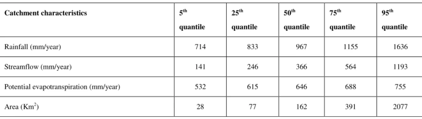
Table 2.1 summarises the variability of rainfall, streamflow, potential evapotranspiration, and
catchment size in the data set.
Table 2.1 Variability in size and the main hydroclimatic conditions over the catchment set
Catchment characteristics 5th quantile 25th quantile 50th quantile 75th quantile 95th quantile Rainfall (mm/year) 714 833 967 1155 1636 Streamflow (mm/year) 141 246 366 564 1193
Potential evapotranspiration (mm/year) 532 615 646 688 755
The variability of mean streamflow values can be expressed as a function of mean P and mean PE. Figure 2.2 plots the runoff coefficient (Q/P) as a function of the aridity index (P/PE) (see Le Moine et al., 2007). It illustrates the variability of hydro-climatic conditions in the test catchments. As explained in details by Le Moine et al. (2007), there are many catchments in this data set for which water losses are greater than PE (points lying below the line y=1−1/x), which may be an indication of leaky catchments. There are also a few catchments for which mean flow is greater than mean rainfall (points above the line y=1), which mainly correspond to catchments with karstic influences, i.e. those fed by inter-catchment groundwater flows from surrounding areas. Even though these catchments may prove more difficult to model, they were not discarded from the data set, as advocated by Andréassian et al. (2010).
Figure 2.2: Mean Q/P vs P/PE values for the catchments in the data set
2.2.2. Sample catchments
It will not be possible to display the detailed results for all catchments. Hence we selected four sample catchments (listed in Table 2.2) representing various conditions. The selection is based on the analysis of some of its flow characteristics such as base-flow index, Q90 (flow equalled or exceeded 90% of the time) and climatic characteristics such as the aridity index.
y=1
Table 2.2: Characteristics of sample catchments
Code in the study A B J K
HYDRO Code A7010610 B2220010 J3205710 K6402510
River Moselle River Meuse River Aber Wrac'h River La Sauldre
Gauging station Custines Saint Michel Drennec Salbris
Area (Km2) 6830 2540 24 1200
Mean flow (mm/y) 530 378 593 232
Mean rainfall (mm/y) 1109 954 1087 825
Mean potential
evapotranspiration (mm/y)
614 619 643 684
Major geology Marnes Massive limestone Crystalline igneous
rocks
Chalks
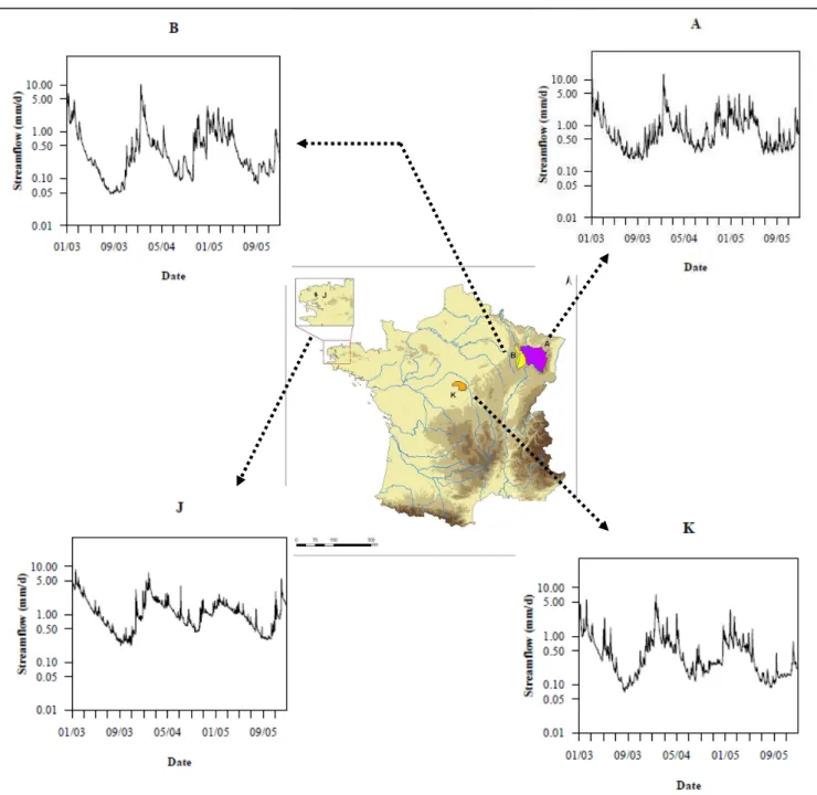
Table 2.2 gives characteristics of the sample catchments. The selected catchments differ in hydro-climatic as well as geologic conditions. Figure 2.3 shows the location and the flow hydrographs of these catchments for a period of three years (2003-2005), in which 2003 and 2005 correspond to two strong drought events in France. To improve the readability of low flows, discharge is plotted on a logarithmic scale.
Figure 2.3: Illustration of location of sample catchments and their daily flow hydrographs from 2003 to 2005
2.3. Low-flow measures
The next sections briefly describe some of the low-flow measures used in this study to characterise low flows in the data set. The values taken by these indices on our catchment set will be discussed in section 2.4.
2.3.1. Low-flow period (low-flow spells)
Low-flow period indicates the period for which stream flows are below a certain threshold. The threshold value depends on the purpose. In France, periods of low flows are critical for managing water resources as the society depends on the availability of water through regulated and unregulated river systems. In regulated river systems, reservoirs make a balance between high and low flows. Hence the knowledge of low-flow period is required by engineers and water managers for their design and also for allocations.
2.3.2. Flow duration curve (FDC)
Flow duration curve is an informative way to display the complete range of discharge, from low flows to flood events. It shows the percentage of time a given flow value is exceeded (Iacobellis, 2008). For more information about FDC, please refer to Vogel and Fennessey (1994). The FDC of sample catchments will be discussed in the later section.
2.3.3. Mean annual minimum flow for different durations
The mean annual minima of flow values can be derived from a daily flow series by selecting the lowest flow every year and calculating the mean. Minima of different durations can be determined, for flows commonly averaged over 1, 3, 7, 10, 30 and 90 days. These low-flow indicators are quite widely used in the water resources evaluation, as discussed in section 2.3.1. Among these, mean annual minimum for a consecutive seven-day period (MAM7) is one of the most commonly used low-flow indices in many countries. It can eliminate the day-to-day variations in the river flow. Smakhtin and Toulouse (1998) also supported the applicability of MAM7 in the UK as abstraction licensing index. QMNA5 is another commonly used low-flow index in France as a policy threshold. It is the minimum annual monthly flow with a return period of five years. In the present study, we consider MAM7 and
QMNA5 to characterise low flows on the study catchments. These minimum values are used
to regulate reservoir operations, irrigation or industrial abstractions, and waste load allocation into streams.
2.3.4. Base-flow index (BFI)
Streamflow hydrograph represents the discharge of the stream as a function of time and it is the combination of different water sources which contributes to the streamflow. The main components which contribute to streamflow are quick flow and base flow. Quick flow is the
direct response to a rainfall event including overland flow (runoff), lateral movement in the soil profile (interflow) and direct rainfall on the stream surface (direct precipitation). Base flow is the delayed discharge from natural storages (groundwater) and it depends on the aquifer characteristics. The groundwater contribution to streams is a critical issue while considering different water management operations. One widely used index to specify the contribution of groundwater to streams is the base flow index (BFI). It is the proportion of base flow in the total runoff. BFI can be used as a descriptor for hydrological modelling, as a tool for selecting analogue catchments, and for estimating annual and long-term groundwater recharge. The literature analysis shows that different methodologies are available to derive the BFI from the streamflow hydrograph (e.g. Nathan and McMahon, 1990; Szilagyi and Parlange, 1998; Furey and Gupta, 2000; Schwartz, 2007; Longobardi and Villani, 2008; Santhi et al., 2008). The present study used the smoothed minima technique (Nathan and McMahon, 1990) to derive the BFI values, because it is easy to implement.
2.4. Computations of low-flow indices on the study catchment set
This section presents a brief description of the computation of the selected low-flow characteristics for the data set.
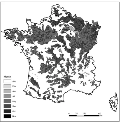
We used the mean monthly minimum streamflow values to characterise the period of occurrence of low flows (Figure 2.4). In most of the catchments, low flows occur during August and September. For a few catchments, low flows occur during November, indicating late flow recessions. In some catchments, low flows occur in February which is typically due to the snow accumulation during winter season.
Figure 2.4: Illustration of the period of occurrence of low-flows in the test data set
The flow duration curve of the sample catchments are presented in Figure 2.5. The flow values (Q) are plotted in a logarithmic scale. The shape of the FDC is quite different between the sample catchments.