HAL Id: hal-01132440
https://hal.archives-ouvertes.fr/hal-01132440
Submitted on 21 Apr 2015
HAL is a multi-disciplinary open access
archive for the deposit and dissemination of
sci-entific research documents, whether they are
pub-lished or not. The documents may come from
L’archive ouverte pluridisciplinaire HAL, est
destinée au dépôt et à la diffusion de documents
scientifiques de niveau recherche, publiés ou non,
émanant des établissements d’enseignement et de
Homological Reconstruction and Simplification in R3
Dominique Attali, Ulrich Bauer, Olivier Devillers, Marc Glisse, André Lieutier
To cite this version:
Dominique Attali, Ulrich Bauer, Olivier Devillers, Marc Glisse, André Lieutier. Homological
Recon-struction and Simplification in R3. Computational Geometry, Elsevier, 2015, 48 (8), pp.606-621.
�10.1016/j.comgeo.2014.08.010�. �hal-01132440�
Homological Reconstruction and Simplification in R
3 Dominique AttaliGipsa-lab, Saint Martin d’Hères, France Ulrich Bauer⇤
IST Austria, Klosterneuburg, Austria Olivier Devillers
INRIA Sophia Antipolis – Méditerranée, Sophia Antipolis, France Marc Glisse
INRIA Saclay – Île-de-France, Orsay, France André Lieutier
Dassault Système, Aix-en-Provence, France
Abstract
We consider the problem of deciding whether the persistent homology group of a simplicial pair (K, L) can be realized as the homology H⇤(X) of some complex X with
L ⇢ X ⇢ K. We show that this problem is NP-complete even if K is embedded in R3.
As a consequence, we show that it is NP-hard to simplify level and sublevel sets of scalar functions on S3within a given tolerance constraint. This problem has relevance
to the visualization of medical images by isosurfaces. We also show an implication to the theory of well groups of scalar functions: not every well group can be realized by some level set, and deciding whether a well group can be realized is NP-hard.
Keywords: NP-hard problems, homology, persistence 2010 MSC: 55U10
⇤Corresponding author.
Email addresses: mail@ulrich-bauer.org (Ulrich Bauer ), Andre.LIEUTIER@3ds.com (André Lieutier)
URL: http://www.gipsa-lab.grenoble-inp.fr/ (Dominique Attali), http://ulrich-bauer.org(Ulrich Bauer ),
http://www-sop.inria.fr/members/Olivier.Devillers/(Olivier Devillers), http://geometrica.saclay.inria.fr/team/Marc.Glisse/(Marc Glisse)
1. Introduction
In this paper, we establish NP-completeness of a variety of related problems that ask for an object in R3with certain prescribed topological constraints.
In the most basic setting, we have a point cloud in Rd that samples a shape and
want to retrieve information on the sampled shape. There exists a whole spectrum of possibilities regarding the type of sought information. At the coarsest level, we can content ourselves with the homology groups which record the “holes” of a given dimension, hereafter referred to as homological features (connected components, cycles, cavities and so on). At a finer level, we may be interested in building an approximation of the shape, reflecting as accurately as possible both its geometry and topology. The standard way is to construct a simplicial complex using the data points as vertices, such as for instance the ↵-complex, the Rips complex or the ˇCech complex [13,12]. All three constructions have in common to depend upon a scale parameter ↵ and to get bigger as ↵ increases. In the ideal case, we expect the complex to have the right homology for some suitable value of ↵ [21,6,7,2]. Unfortunately, depending on the sampling, it may happen that such a value of ↵ does not exist. Nonetheless, we might still be able to infer the true homology of the shape hidden in the noisy data using persistent homology [15,10,8]. Given two scale parameters ↵1 and ↵2, the persistent homology groups
record the homological features that persist from ↵1to ↵2. Under very weak hypotheses,
we know that the persistent homology is precisely that of the sampled shape [10,5]. The persistent homology can be computed efficiently (i.e., in polynomial time).
A natural question is then to ask for a complex that carries the persistent homology: given a complex K and a subcomplex L, can we find a subcomplex of K that contains L and whose homological features are precisely those common to L and K? Our answer is that sometimes we cannot, and deciding whether we can is NP-complete. This answer was first given in the general case by Attali and Lieutier [1], who posed the restriction to complexes embedded in R3as an open problem. We resolve this problem by proving
NP-completeness even for complexes embedded in R3.
The above problem concentrates on building a complex whose homology matches perfectly the persistent homology of L into K: all the homological noise has been removed. We call such an object a homological reconstruction. However, when it does not exist, it is still relevant to look for a complex nested between L and K and whose homology is as close as possible to the persistent homology of L into K: as much noise as possible has been removed. We call such a complex a homological simplification and prove that finding one is also an NP-hard problem.
In the field of visualization and image analysis, another common setting consists in describing a shape through a continuous function f : Rd! R instead of a point cloud
in Rd. For instance, a medical image may be a collection of density measurements over
a grid of 3D points and is best modeled as a continuous map over a certain domain of R3.
In the ideal case, the shape is a sublevel set of the function, f 1( 1, t]. Unfortunately,
noise can plague the data. As the parameter t increases, sublevel sets inflate and we can track the evolution of their homology. Features that appear and disappear quickly are considered topological noise, and we can consider the common features of two sublevel sets as those of a denoised sublevel set. The question now becomes: can we find another cleaner function, close enough to the original one, whose sublevel set has the
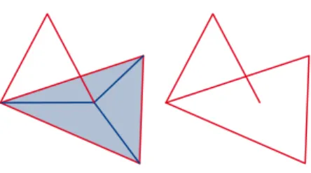
Figure 1: Example of a simplicial pair (K, L) embedded in R3that has no homological reconstruction.
denoised homology, i.e., a sublevel set reconstruction? The corresponding optimization problem asks for a sublevel set simplification, i.e., a function close to the original one that minimizes the number of homological features of the sublevel set. We show that these two problems are the equivalents in the functional setting to the homological reconstruction and simplification of simplicial pairs described above.
Often, one is also interested in the homology of a level set, f 1(t). We show
how it can be related to the (persistent) homology of sublevel sets, and consider the corresponding level set reconstruction/simplification problems.
Further in this direction, Edelsbrunner et al. introduced the well group [16,3] as a denoised version of the homology group of a level set. Again, we can ask whether one can find a realization of the well group, i.e., a cleaner function whose level set has the same homology as the well group?
We shall see in this paper that all of these related problems are NP-hard, as a consequence of the NP-completeness of the homological reconstruction problem. 1.1. Background and notations
We are only concerned with topological spaces that are triangulable by a finite simplicial complex, so simplicial and singular homology are isomorphic and we make no distinction between the two. In particular, we use the simplicial versions of the Excision and Mayer-Vietoris sequence theorems, which have less restrictive assumptions than their singular counterparts. If K is an abstract simplicial complex, we denote by K its geometric realization. Throughout this article, we consider homology with coefficients in an arbitrary field F, so the homology groups are finite-dimensional F-vector spaces and there is no torsion. Note that for simplicial complexes K embedded in R3, this is
in fact not a restriction, since due to the absence of torsion in R3the Betti numbers are
independent of the choice of coefficients (see, e.g., [17, §3.3]).
Given a topological space K, we write H⇤(K) =LiHi(K) for the direct sum of
homology groups in all dimensions, and (K) =Pi 0 i(K) for the total Betti number.
If (K, L) is a pair of topological spaces L ⇢ K, the inclusion L ,! K induces a homomorphism H⇤(L) ! H⇤(K), which is denoted by H⇤(L ,! K). The rank of
this map is the persistent Betti number of the inclusion L ,! K and is denoted by (L ,! K) = rank H⇤(L ,! K); the image im H⇤(L ,! K) is a persistent homology
group. If (K, L) is a simplicial pair, that is, a pair of simplicial complexes such that L ⇢ K, then the persistent Betti number (L ,! K) can be computed in time cubic in
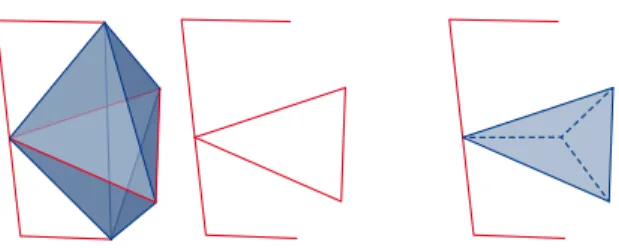
Figure 2: Example of a simplicial pair (left) having a homological reconstruction as a subspace (right), but not as a subcomplex. The simplicial complex on the left contains three tetrahedra sharing an edge and whose union forms a triangular bipyramid.
the number of simplices in K [15]. This cubic complexity can be improved to matrix multiplication time [19].
A piecewise linear function on a topological space K is a continuous function f : K ! R such that there exists a finite triangulation of K on which f is simplexwise linear. Note that a simplexwise linear function must be linear on each simplex of the given triangulation, while a piecewise linear function is linear on each simplex of some arbitrary triangulation.
2. Reconstruction and simplification of simplicial pairs
In this section, we consider a simplicial pair and define the homological reconstruc-tion problem and the homological simplificareconstruc-tion problem. We prove that both problems are NP-hard when the simplicial pair is embedded in R3. We start with a simple lemma:
Lemma 1. Consider a triple of topological spaces L ⇢ X ⇢ K with finite Betti numbers. Then
(X) (L ,! K).
Proof. This is a consequence of the fact that whenever we consider two linear maps j : U ! V and i : V ! W between finite dimensional vector spaces, then dim V
rank j rank i j. ⇤
This property suggests the following definition:
Definition 1. Consider a triple of topological spaces L ⇢ X ⇢ K with finite Betti numbers. Then X is called a homological reconstruction of (K, L) if (X) = (L ,! K). Moreover, X is called a homological p-reconstruction of (K, L) if p(X) = p(L ,! K).
We will often omit “homological” since there is no ambiguity in this paper. An equivalent condition for X being a reconstruction is that H⇤(L ,! X) is surjective and
H⇤(X ,! K) is injective, as defined in [1]. Not every pair (K, L) admits a reconstruction;
a simple counterexample is shown in Fig.1. The use of topological spaces in the definition (as opposed to simplicial complexes) is motivated by the following observation. Let (K, L) be a simplicial pair. Then there might be a reconstruction of (K, L), but not as a subcomplex of K. An example is shown in Fig.2. A reconstruction that is a
subcomplex is called a subcomplex reconstruction. To emphasize the distinction to this case, we sometimes use the term subspace reconstruction to emphasize that the reconstruction is only required to be a subspace, not necessarily a subcomplex. 2.1. Homological reconstruction is NP-hard
We now focus our attention on spaces that are geometric realizations of finite simplicial complexes embedded in R3.
Theorem 1. The homological reconstruction problem is NP-hard: Given as input a simplicial pair (K, L) embedded in R3, decide whether there exists a subspace
recon-struction X of (K, L). The problem is NP-complete if X is required to be a subcomplex. This section is devoted to the proof of Theorem1by reduction from 3-SAT. Recall that a Boolean formula is in 3-CNF if it is a conjunction of several clauses, each of which is a disjunction of three literals, a literal being either a variable or its negation. Given a 3-CNF formula , we construct a simplicial pair (K , L ) embedded in R3and
prove that (K , L ) has a reconstruction (as a subcomplex of K ) if and only if has a satisfying assignment (see Lemmas2and3below).
For this, we associate to the 3-CNF formula a simplicial pair (K , L ) with trivial persistent homology. Equivalently, any reconstruction X of (K , L ) has trivial homology, i.e.,
d(X) = d(L ,! K ) =
8 >><
>>:1 if d = 0,0 otherwise.
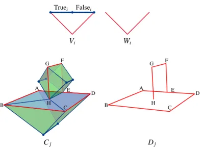
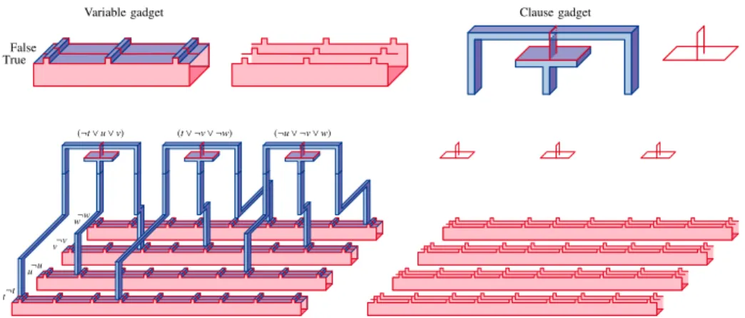
This means that X has a single connected component, no loops, and no cavities. X has to fill all loops or cavities in L and has to connect the di↵erent connected components of L by adding to L portions of K without creating any new loops or cavities. The variable gadget. The variable gadget is a simplicial pair (Vi,Wi) as depicted in
Fig.3, top. The simplicial complex Vicontains 4 edges forming a cycle. The two bold
edges do not belong to Wi. One of the bold edges will be called Trueiand the other one
will be called Falsei. The key property of this construction is that any reconstruction of
the pair (Vi,Wi) cannot contain both edges Trueiand Falsei, for otherwise they would
form a 1-cycle with the remaining edges. This property will allow us to match the presence of the edge Trueito a true assignment of the variable vi.
The clause gadget. The clause gadget is a simplicial pair (Cj,Dj) as depicted in Fig.3,
bottom. The simplicial complex Djcontains a cycle ABCDE. The cycle is closed with
two surfaces in Cj(thereafter referred to as the lower hemisphere and the disk) thereby
creating a cavity. Furthermore, the complex Djcontains an arc that ends inside the disk.
Whenever we fill the cycle ABCDE with the disk, this connects the two endpoints of the arc, thus creating a new cycle, which we close twice in Cjby a left hemisphere and a
right hemisphere. Consider one bold edge in the interior of each hemisphere, which is where the clause gadget will connect to the variable gadgets.
The key property of this clause gadget is that at least one of the 3 bold edges must be present in any reconstruction X of the pair (Cj,Dj). Indeed, the cycle ABCDE in X
Truei Falsei Vi Wi A B C D E F G H A B C D E F G H Cj Dj
Figure 3: Variable (top) and clause (bottom) gadgets for the reduction of homological reconstruction to 3-SAT.
the disk, we have a new cycle EFGH in X which in turn must be killed either by the left or by the right hemisphere. In any case, X contains at least one of the hemispheres and thus one of the three bold edges.
Correspondence with a formula. Given a 3-CNF formula with n clauses c1, . . . ,cn
and m variables v1. . . ,vm, we construct a 2-dimensional pair (K , L ) as follows. For
each variable viwe take a copy (Vi,Wi) of the variable gadget. For each clause cj, we
take a copy (Cj,Dj) of the clause gadget; for each literal eviof cj, we identify one of
the bold edges of Cjto Falseiif e is a negation and Trueiotherwise. See Fig.4for an
example.
First notice that 2(L ) = 0 (i.e., L has no cavities). Second, we can assume that 0(K ) = 1 (i.e., K is connected). Indeed, if K is disconnected, it means that the
3-SAT problem (and the reconstruction problem) can be decomposed into 2 independent subproblems with disjoint sets of variables, which can be solved separately. Last,
1(L ,! K ) = 0 (i.e., the cycles in L are boundaries in K ). Indeed, the only
1-cycles in L are the 1-cycles ABCDE in each Dj, and they are filled in K . This
means that we are looking for a reconstruction with trivial homology.
From a reconstruction to a satisfying assignment. Let X be a homological reconstruc-tion of the pair (K , L ). We do not assume that X is the geometric realizareconstruc-tion of some subcomplex of K . Assign to each variable vithe value true if the edge Trueiis entirely
contained in X, and false otherwise. For each clause gadget (Cj,Dj), at least one bold
edge is contained in X. If this edge corresponds to a positive literal vi, this means that
Trueiis in X, viis true and the clause is satisfied. If the edge corresponds to a negative
literal ¬vi, this implies that Falseiis in X. Trueiis thus not in X, so viwas assigned
false and the clause is satisfied. We have thus shown that the assignment of the variables makes the formula evaluate to true:
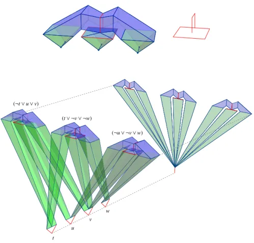
(¬t _ u _ v) (t _ ¬v _ ¬w) (¬u _ ¬v _ w) t u v w
Figure 4: Embedding of the clause gadget with aligned hemispheres (top), and the simplicial complex K generated in the reduction from the 3-SAT instance (¬t ^ u ^ v) _ (t ^ ¬v ^ ¬w) _ (¬u ^ ¬v ^ w) (bottom left), with parallel projection (bottom right) orthogonal to the alignment axis of the variable gadgets.
Lemma 2. If (K , L ) has a homological reconstruction, then has a satisfying assignment.
From a satisfying assignment to a reconstruction. Given a satisfying assignment for the formula , we construct a subcomplex reconstruction X of (K , L ). We start with X = L and add to X a selected set of simplices from K . For each clause cj, we pick
one literal that evaluates to true and close the cycle in the clause gadget complex Dj
correspondingly. If the literal corresponds to the bold edge of the lower hemisphere, we add this hemisphere. Otherwise, we add the disk and the hemisphere that contains the bold edge corresponding to the selected literal.
The only 2-cycles in K are in the clause gadgets. As we did not create any 2-cycle in X, it follows that 2(X) = 0. By construction, filling the clause gadgets never introduced
both Truei and Falseiin X. Indeed, it could only introduce Trueiif viwas assigned
the variable gadgets do not appear in X. Also, for each clause gadget, we filled the ABCDE 1-cycle, and whenever we created an extra EFGH 1-cycle by adding the disk, we immediately filled it with the left or right hemisphere. Now we only need to check that the construction did not create any “non-local” 1-cycles. Since for each clause we have only used one of the literals which evaluate to true, the only contact a clause gadget in X has with the rest of X is through a single bold edge, and the clause gadget can be collapsed to that edge. After collapsing all clause gadgets, all that remains are disconnected variable gadgets with at most 3 edges each, and so 1(X) = 0. We finally
add to X just enough edges from K so that it becomes connected, without creating any extra cycles in the process. This is possible since we assumed that K is connected. Thus we have 0(X) = 1. We conclude:
Lemma 3. If has a satisfying assignment, then (K , L ) has a subcomplex recon-struction.
We are now in a position to prove Theorem1.
Proof of Theorem1. First we show that the homological reconstruction problem is NP-hard. We proceed by reduction from 3-SAT. Let (K, L) = (K , L ) be a simplicial pair defined by a 3-SAT instance . We show that the following propositions are equivalent: (a) (K, L) has a subspace reconstruction;
(b) has a satisfying assignment;
(c) (K, L) has a subcomplex reconstruction.
The implication (a) =) (b) is shown in Lemma2; (b) =) (c) is shown in Lemma3. Finally, (c) =) (a) is trivial.
The pair (K, L) can be constructed from in time polynomial in the size of . To-gether with the equivalence (a) () (b), this establishes NP-hardness of the homological reconstruction problem.
The equivalence (b) () (c) also yields NP-hardness of the subcomplex reconstruc-tion problem. Moreover, given a subcomplex X as a polynomial size certificate, we can decide in polynomial time whether X is a reconstruction of (K, L). Thus the problem is
also in NP and hence NP-complete. ⇤
Embedding. Later, we have to consider not only an embedding of K , but also a triangulation of its complement. The following fact will be useful:
Lemma 4. There is a triangulation of S3with size polynomial in the size of K and
having K as a subcomplex.
Proof. First, referring to Fig.4, it is clear that K can be embedded in R3. Indeed, we
can align the clause gadgets and the variable gadgets along two lines parallel to the coordinate axes and make each clause gadget look like a small body with three long tentacles that connect to the variable gadgets. Due to the way the variable and clause gadgets are aligned in the construction along skew axes, the tentacles do not intersect in their interior.
Variable gadget TrueFalse Clause gadget ¬t t ¬u u ¬v v ¬w w (¬t _ u _ v) (t _ ¬v _ ¬w) (¬u _ ¬v _ w)
Figure 5: Example of 3-SAT reduction using a 3D grid embedding.
We can subdivide the space by first projecting K onto a plane orthogonal to the line carrying the variable gadgets. We get a polygonal region whose complement can easily be triangulated inside a bounding box without adding any new vertex and thus adding a linear number of edges. Extending each triangle in the direction of the projection, we get a collection of tubes, one for each triangle. The tubes can easily be triangulated while respecting K to obtain a polynomial size triangulation of a bounding box of the construction, which can trivially be extended to a polynomial size triangulation
of S3. ⇤
We want to remark that a similar construction can be realized even if we restrict edges and faces of L and K to be edges and faces of a 3D grid (see Fig.5). This means that a variant of Theorem1can also be shown for cubical complexes arising from 3D image data.
Corollary 1. The homological simplification problem is NP-hard: Given as input a simplicial pair (K, L) embedded in R3, find a complex X minimizing (X) subject to
L ⇢ X ⇢ K.
Proof. We use a reduction from the subcomplex reconstruction problem. To determine if a subcomplex reconstruction exists, we can first find a complex X minimizing (X) subject to L ⇢ X ⇢ K. We then only need to check if its Betti number matches the lower
bound (L ,! K). ⇤
3. Reconstruction and simplification of level and sublevel sets
In this section, we consider a real-valued simplexwise linear function defined on a simplicial complex embedded in R3and establish the NP-hardness of problems that ask
for a nearby function with a simplified sublevel set (Section3.1) and a simplified level set (Section3.3).
Given a real-valued function f , we write Ft for the t-level set f 1(t), Ftfor the
(closed) t-sublevel set f 1(( 1, t]), and F
–2 0 0 0 –2 –2 –2 –2 –2 –2 –2 0 –2 –1 –1 –1 –2 –2 –2 –2 –2 –2 –2 1
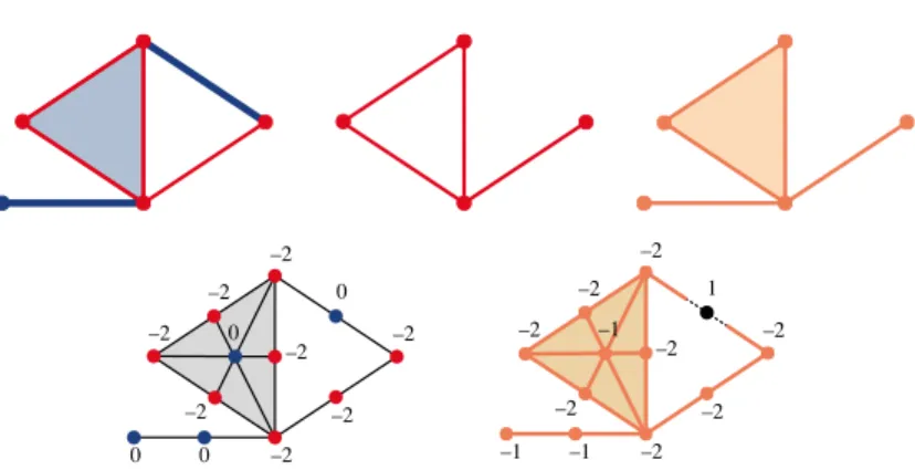
Figure 6: Top: A simplicial pair (K, L) and a homological reconstruction of (K, L) as a subcomplex. Bottom: values of f (left) and g (right) at the vertices of the barycentric subdivision sd K, as used in the proof of Theorem2.
this paper we shall only consider real-valued piecewise linear functions. Note that level and sublevel sets of a simplexwise linear function on a simplicial complex K are not necessarily subcomplexes of K, but subcomplexes of an appropriate subdivision of K. Moreover, we have the following property:
Proposition 1 (Kühnel [18], Morozov [20]). Let f be a simplexwise linear function on a simplicial complex K. Let K(t) be the induced subcomplex of K on {v 2 vert K :
f (v) t}. Then K(t) is homotopy equivalent to the sublevel set Ft. If t , f (v) for all
v 2 vert K, then K(t) is also homotopy equivalent to the open sublevel set F<t.
Definition 2. Let f , g be piecewise linear functions and consider real parameters t and . The function g is called a sublevel set (t, )-reconstruction of f if kg f k1 and
Gtis a reconstruction of the pair (Ft+ ,Ft ), i.e.,
(Gt) = (Ft ,! Ft+ ).
Note that
Ft ✓ Gt✓ Ft+ ,
so that
(Gt) (Ft ,! Ft+ ).
A sublevel set (t, )-reconstruction is thus also a minimizer of (Gt) subject to kg
f k1 .
3.1. Sublevel set reconstruction is NP-hard
Theorem 2. The sublevel set reconstruction problem is NP-hard: Given as input a simplexwise linear function f on a simplicial complex embedded in R3and parameters
Proof. It suffices to establish the theorem for t = 0 and = 1. We proceed by reduction from 3-SAT using the results of the previous section. Let (K, L) = (K , L ) be a simpli-cial pair defined by a 3-SAT instance , as described in the proof of Theorem1. We construct an instance of the level set simplification problem by defining a simplexwise linear function f : sd K ! R on the barycentric subdivision of K; see Figure6. Recall that the barycentric subdivision (or derived subdivision) of a simplicial complex K is the order complex of the face relation, i.e., the abstract simplicial complex sd K whose vertices are the simplices of K and whose simplices are the totally ordered subsets of K with regard to the face relation. We define f via its values on the vertices of sd K. Using the fact that a vertex of sd K is a simplex of K, we let
f : 7! 8 >><
>>:02 ifotherwise.2 L, (1) Note that for every function g with kg f k1 1, the 0-sublevel set G0contains
L and is contained in K. We show that the following propositions are equivalent to propositions (a)–(c) in the proof of Theorem1:
(d) f has a simplexwise linear sublevel set (0, 1)-reconstruction g. (e) f has a sublevel set (0, 1)-reconstruction g.
To show (c) =) (d), we define a simplexwise linear function g on sd K by its values on the vertices of sd K (the simplices of K); see Figure6:
g : 7! 8 >>>>> < >>>>> : 2 if 2 L, 1 if 2 X \ L, 1 if 2 K \ X. (2) We have kg f k1=1. By Proposition1, the sublevel set G0is homotopy equivalent
to |X| and hence is a reconstruction of the pair (K, L) ' (F1,F 1).
Finally, (d) =) (e) is trivial and (e) =) (a) follows directly with G0as a reconstruction
of (F1,F 1) ' (K, L).
The function f can be constructed from the 3-SAT instance in polynomial time. Together with the equivalence (b) () (e), this establishes NP-hardness of the sublevel set reconstruction problem.
The equivalence (b) () (d) also yields NP-hardness of the sublevel set reconstruc-tion problem restricted to simplexwise linear funcreconstruc-tions sd K ! R. ⇤ Theorem 3. The sublevel set reconstruction problem is NP-complete if the reconstruc-tion is required to be simplexwise linear on the same complex.
Proof. By Theorem2, it is sufficient to show that the problem is in NP, i.e. every “yes” instance f : K ! R has certificate with size polynomial in the size of K and f . Again, it suffices to establish the theorem for t = 0 and = 1. We show that there is
a simplexwise linear (0, 1)-reconstruction g i↵ there is a subset of vertices S whose induced subcomplex KS is a reconstruction of (K(1), K( 1)), where K(t) is the induced
subcomplex of K on {v 2 vert K : f (v) t} as in Proposition1.
The subset of vertices v with g(v) 0 induces a subcomplex that is homotopy equivalent to the sublevel set G0, by Proposition1. Vice versa, let S be a subset of
vertices such that the induced subcomplex KS is a reconstruction of (K(1), K( 1)). In
particular, for all v 2 S we have f (v) 1, and for all v < S we have f (v) > 1. Define a simplexwise linear function by the vertex values
h : v 7! 8 >><
>>:f (v) 1 if v 2 S,f (v) + 1 if v < S,
and note that for each vertex v, h(v) 0 if and only if v 2 S . By Proposition1, the sublevel set H0 is homotopy equivalent to the induced subcomplex KS and hence
is a reconstruction of the pair (F1,F 1) ' (K(1), K( 1)). We conclude that h is a
(0, 1)-reconstruction of f .
Given a subset S as a polynomial size certificate, by computing and comparing (KS)
and (K( 1) ,! K(1)) we can verify in polynomial time the existence of a sublevel set (0, 1)-reconstruction of f . Thus the problem is also in NP and hence NP-complete. ⇤ Corollary 2. The sublevel set simplification problem is NP-hard: Given as input a simplexwise linear function f on a simplicial complex embedded in R3and parameters
t and , find a simplexwise linear function g minimizing (Gt) subject to kg f k1 .
Proof. We use a reduction from the sublevel set reconstruction problem. To determine if f has a sublevel set (t, )-reconstruction, we can first find a simplexwise linear minimizer of (Gt). We then only need to check if (Gt) matches the lower bound
(Ft ,! Ft+ ),
which can be done in time polynomial in the size of K. ⇤ 3.2. Betti numbers of level and sublevel sets
The Betti numbers of level and sublevel sets are related by the following formula: Lemma 5. Let f be a piecewise linear function on Sn, n > 1, and let t be in the interior
of the image of f , t 2 int(im f ). Then
d(Ft) = d(Ft) + n d 1(F<t).
Proof. First recall that Ft, F t, and F tare subcomplexes of an appropriate
triangula-tion of Sn, so we can apply the simplicial version of the Mayer-Vietoris theorem [22,
§4.6]. By exactness of the Mayer-Vietoris sequence for Sn, F
t, and F t, we have [14] d(Ft) = d(Ft) + d(F t) + 8 >>>>> < >>>>> : 1 if d = 0, 1 if d = n 1, 0 otherwise. (3)
By Alexander duality [17, §3.3], the duality of homology and cohomology with field coefficients resulting from the universal coefficient theorem [17, §3.1], and isomorphism of dual finite-dimensional vector spaces, we have
e
Hd(F t) Hen d 1(F<t) Hom( eHn d 1(F<t), F) Hen d 1(F<t),
where eHddenotes the dth reduced homology group and Hom( eHn d 1(F<t), F) is the dual
vector space of eHn d 1(F<t), i.e., the linear maps to F. Recall that d(X) = rank( eHd(X)) + 8 >>< >>:1 if d = 0,0 otherwise. We thus have d(F t) = n d 1(F<t) + 8 >>>>> < >>>>> : 1 if d = 0, 1 if d = n 1, 0 otherwise. (4) By combining Eqs. (3) and (4), we obtain the stated equality. ⇤
For all piecewise linear functions f, g on Snwith kg f k
1 and t ± 2 int(im f ),
we have t 2 int(im g) and thus by Lemmas1and5,
(Gt) (Ft ,! Ft+ ) + (F<t ,! F<t+).
This motivates the following definition:
Definition 3. Let f , g be piecewise linear functions on Snand consider real parameters
t and with t ± 2 int(im f ). The function g is called a level set (t, )-reconstruction of f if kg f k1 and
(Gt) = (Ft ,! Ft+ ) + (F<t ,! F<t+).
A level set (t, )-reconstruction is thus also a minimizer of (Gt) subject to kg f k1
. Since the above equality can only be achieved if both inequalities (Gt) (Ft ,! Ft+ ) and
(G<t) (F<t ,! F<t+)
derived from Lemma1hold with equality, we conclude:
Lemma 6. Let f , g be piecewise linear functions on Sn. If g is a level set (t,
)-reconstruction of f , then
(Gt) = (Ft ,! Ft+ )
(G<t) = (F<t ,! F<t+)
and in particular g is also a sublevel set (t, )-reconstruction of f .
We will show in the following that sublevel set reconstructions are also level set reconstructions, under some additional hypotheses.
3.3. Level set reconstruction is NP-hard
Definition 4. Let f be a piecewise linear function. A homological regular value of f is a number t 2 R such that H⇤(F<t,! Ft) is an isomorphism.
We remark that there exist several other notions of regularity in the literature, which do not match our definition when extended to general functions [10,4]. For piecewise linear functions however, all these definitions are equivalent. Note also that regularity should be understood with respect to sublevel sets; t can be a regular value t even though H⇤(F>t,! F t) might not be an isomorphism.
Lemma 7. Let f be a piecewise linear function on Sn, n > 1. If t ± 2 int(im f ) are
regular values of f and g is a level set (t, )-reconstruction of f , then t is a regular value of g.
Proof. By hypothesis t ± are regular values of f , so
H⇤(F<t ,! Ft ) and H⇤(F<t+ ,! Ft+ )
are isomorphisms and
(F<t ,! F<t+) = (F<t ,! Ft+ ) = (Ft ,! Ft+ ).
Since g is a level set (t, )-reconstruction of f , by Lemma6, we have (Gt) = (Ft ,! Ft+ ) and (G<t) = (F<t ,! F<t+) and hence (Gt) = (G<t) = (F<t ,! Ft+ ). Observing that F<t ⇢ G<t⇢ Gt⇢ Gt+
and using the fact that whenever we have three linear maps U ! V ! W ! X between finite-dimensional vector spaces, then
rank(U ! X) rank(V ! W), we get
(F<t ,! Ft+ ) (G<t,! Gt) (Gt).
Combining all these relations, we deduce that
(Gt) = (G<t) = (G<t,! Gt) = (Gt).
Lemma 8. Let f and g be piecewise linear functions on Sn, n > 1. Assume that
t ± 2 int(im f ) are regular values of f and t 2 int(im g) is a regular value of g. Then g is a sublevel set (t, reconstruction of f if and only if g is a level set (t, )-reconstruction of f .
Proof. By hypothesis, t is a regular value of g. Substituting into Lemma5, we obtain the first equation below; the second equation comes from the fact that t ± are regular values of f :
2 (Gt) = (Gt),
2 (Ft ,! Ft+ ) = (Ft ,! Ft+ ) + (F<t ,! F<t+).
By definition, g is a sublevel set (t, )-reconstruction of f if and only if the left hand sides of the two equations above are equal. Similarly, g is a level set (t, )-reconstruction if and only if the right hand sides of the two equations above are equal. The result
follows immediately. ⇤
Theorem 4. The level set reconstruction problem is NP-hard: Given as input a simplex-wise linear function on a triangulation of S3and parameters t and , decide whether
there exists a level set (t, )-reconstruction g of f . The problem is NP-complete if g is required to be simplexwise linear on this triangulation.
Proof. We reuse the same reduction as in Theorem2. Since we need functions defined on the sphere, we triangulate the complement of K to obtain a triangulation S of the sphere with size polynomial in the size of K and K ⇢ S as in Lemma4. We extend f from Eq. (1) to a simplexwise linear function ˜f on sd S :
˜f : 7! 8 >><
>>:2f ( ) ifotherwise.2 K,
We then prove that propositions (a)–(e) in the proofs of Theorems1and2and (f), (g) below are equivalent.
(f) ˜f has a simplexwise linear level set (0, 1)-reconstruction ˜g. (g) ˜f has a level set (0, 1)-reconstruction ˜g.
We trivially have (f) =) (g). Now we prove that (g) =) (d). Proposition1implies that the values ±1 are regular values of ˜f. By Lemma7, the value 0 is a regular value of ˜g. Lemma8then proves that ˜g is a sublevel set reconstruction of ˜f. Now let g be the restriction of ˜g to K. Since the sublevel sets Ftand eFtare homotopy equivalent for
t 1, and the sublevel sets Gtand eGtare homotopy equivalent for t 0, it follows
that g is a sublevel set reconstruction of f .
Next, we prove that (c) =) (f). Given a subcomplex reconstruction X of (K, L), we define g using Eq. (2) and extend it to ˜g : sd S ! R as above for ˜f. Since 0 is a regular value of ˜g, Lemma8implies that ˜g is a level set reconstruction.
In analogy to the proof of Theorem2, we obtain NP-hardness of the level set reconstruction problem and NP-completeness of the problem restricted to simplexwise
Corollary 3. The level set simplification problem is NP-hard: Given a piecewise linear function f on S3and parameters t and , find a simplexwise linear function g minimizing
(Gt) subject to kg f k1 .
Proof. To determine if f has a level set (t, )-reconstruction, we can first find a minimizer of (Gt). We then only need to check if (Gt) matches the lower bound
(Gt) = (Gt) + (G<t) (Ft ,! Ft+ ) + (F<t ,! F<t+),
which can be done in time polynomial in the size of the underlying triangulation. ⇤ 4. Realizations of well groups
We now discuss how the previous results relate to the concept of well groups, which were introduced in [16] as a robust version of the homology group of a level set.
Let f : K ! R be a piecewise linear function. For 0 and an interval [a, b] ⇢ R , the ([a, b], )-well group of f is defined as
W⇤( f, [a, b], ) =
\
g:kg f k1
im H⇤(G[a,b],! F[a ,b+ ]),
where F[a,b]= f 1([a, b]). In fact, as shown in [3], the well group is already given by the intersection of just two persistent homology groups:
W⇤( f, [a, b], ) = im H⇤(F[a ,b ],! F[a ,b+ ])
\ im H⇤(F[a+ ,b+ ],! F[a ,b+ ]). (5)
The following formula expresses the rank of the well group in terms of persistent Betti numbers using relative homology.
Theorem 5 (Bendich et al. [3]). Let f : K ! R be a piecewise linear function and let a b and 2 R be such that a ± , b ± are regular values of f . Then
rank W⇤( f, [a, b], ) = (Fb ,! Fb+)
((Fb ,;) ,! (K, F a+))
+ ((K, F a+) ,! (K, F a ))
((Fb+,;) ,! (K, F a )).
We are particularly interested in the case where the interval consists of a single point. We call W⇤( f, t, ) = W⇤( f, [t, t], ) the (t, )-well group of f . Intuitively, it captures the
homology common to all perturbed level sets.
Clearly, the rank of the well group provides a lower bound on the Betti number of the t-level set of any g with kg f k1 :
(Gt) (Gt,! F[t ,t+ ]) rank W⇤( f, t, ).
We say that the well group is realized by such a function g if (Gt) = rank W⇤( f, t, ),
or equivalently, if H⇤(Gt,! F[t ,t+ ]) maps H⇤(Gt) bijectively to W⇤( f, t, ). As we will
show in Theorem6, this lower bound cannot always be achieved, and hence not every well group is realizable.
4.1. Realizability of well groups is NP-hard
We now show that on Sn, a realization of a well group is the same as a level set
reconstruction:
Theorem 6. Let f be a piecewise linear function on Sn with t ± 2 int(im f ). A
piecewise linear function g realizes the well group W⇤( f, t, ) if and only if it is a level
set (t, )-reconstruction of f .
Proof. The number of critical values of f is finite, and so for every s 2 R, there is ✏ > 0 such that all values in [s ✏, s) and in (s, s + ✏] are regular, and hence
H⇤(Fs ✏ ,! F<s) and H⇤(Fs,! Fs+✏)
are isomorphisms. Choose ✏ such that the above holds for s = t ± . Let a = t ✏ and b = t + ✏. Now a ± , b ± are regular values and we can apply Theorem5.
The second and forth terms in the formula of Theorem5vanish. To see this, note that t ± 2 int(im f ) implies
Fb± =Ft+✏± ( Sn
for ✏ small enough, and thus n(Fb±) = 0. Similarly,
F a± =F t ✏± ,;
and thus 0(Sn,F a±) = 0. Moreover, d(Sn) = 0 for d < {0, n}. Since the induced
homomorphisms H⇤((Fb±,;) ,! (Sn,F a⌥ )) factor as H⇤(Fb±) ! H⇤(Sn) ! H⇤(Sn,F a⌥ ), we have ((Fb±,;) ,! (Sn,F a⌥ )) = 0.
Moreover, by the duality theorem of extended persistence on manifolds [11], we can rewrite the third term in Theorem5as
d((Sn,F a+) ,! (Sn,F a )) = n d(Fa ,! Fa+).
Finally, by regularity of the values [a± , t± ) and (t± , b± ], we have isomorphisms H⇤(Ft± ,! F[a± ,b± ]) and H⇤(F[t ,t+ ],! F[a ,b+ ])
and thus by Eq. (5)
W⇤( f, t, ) W⇤( f, [a, b], ).
Altogether, this yields
rank W⇤( f, t, ) = (Ft ,! Ft+ ) + (F<t ,! F<t+ ).
The statement now follows directly from the definitions. ⇤ Together with Theorem4, we have:
Corollary 4. The well group realization problem is NP-hard: Given a piecewise linear function f : K ✓ S3 ! R and parameters t and , decide whether the well group
W⇤( f, t, ) can be realized. The problem is NP-complete if the realization is required to
5. An easy case
In this section, we discuss an important special case in which the subcomplex reconstruction problem can in fact be solved in polynomial time.
5.1. Building a p-reconstruction of an easily p-reconstructible pair
We start by presenting a polynomial time algorithm which outputs a p-reconstruction of the pair (K, L), assuming that (K, L) is p-reconstructible and enjoys an easiness property that we describe below.
Definition 5. Given a simplicial complex K and a subcomplex L, we say that (K, L) is an easily p-reconstructible pair if
(a) (K, L) is p-reconstructible and
(b) for all subcomplexes X such that L ✓ X ✓ K, the homomorphism Hp 1(X ,! K)
induced by the inclusion X ✓ K is injective.
Condition (b) is equivalent to requiring that for every filtration F containing the two simplicial complexes L and K, no (p 1)-cycle is destroyed in F between L and K. In other words, each time a p-simplex is added in F between L and K, it creates a p-cycle; see Figure7. Using the terminology in [15], this means that the filtration F has only positive p-simplices in K \ L. Note that for condition (b) to hold we only need the positivity of p-simplices in K \ L for one filtration F and not for every permutation. To see this, recall that given a filtration F there exists a pairing between its positive
p-simplices and negative (p + 1)-simplices. The analysis in [9] shows that when we swap two consecutive simplices in the filtration, either they keep their pairings, or they swap them, but in no case can the number of negative p-simplices change. It follows that we can go from one filtration F containing L and K to any other while preserving the positivity of p-simplices in K \ L. Hence, checking condition (b) boils down to computing the pairing of p-simplices in F and thus takes polynomial time. In practice, checking the easiness property will not be necessary, as we shall see below.
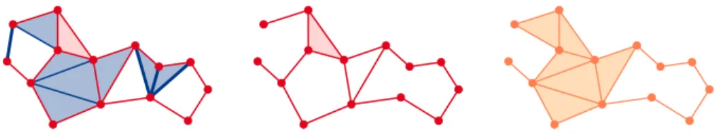
Figure 7: An easily 1-reconstructible pair (K, L) embedded in R2and a 1-reconstruction obtained after
removing from K the (K, L)-homology generating edges (bold edges) and their cofaces.
We now describe a polynomial time algorithm that constructs a solution to the dimension p reconstruction problem of the pair (K, L), whenever (K, L) is easily p-reconstructible. The idea is to remove p-simplices from K in order to “break” p-cycles in K that do not correspond to cycles in L; see Figure7.
We say that a p-simplex 2 K \ L is (K, L)-homology generating if there is a chain c 2 Cp(L) such that @ = @c and [ + c]K< im Hp(L ,! K). Clearly, this implies that
cannot be contained in any homological reconstruction X of (K, L), and hence the same is also true for every coface of . Writing stK for the set of cofaces of in K,
we conclude:
Lemma 9. Let X be a solution to the dimension p reconstruction problem of the pair (K, L). For any (K, L)-homology generating p-simplex , we have stK ✓ K \ X.
This lemma suggests the following algorithm for computing a p-reconstruction of an easily p-reconstructible pair (K, L):
Reconstruction(K, L, p) K0 K
while9 a (K0,L)-homology generating p-simplex
remove stK0 from K0
endwhile returnK0
We now show correctness of the algorithm.
Lemma 10. Suppose (K, L) is an easily p-reconstructible pair. For any (K, L)-homology generating p-simplex , the pair (K0,L), where K0 = K \ stK , is an
easily p-reconstructible pair. Moreover, every p-reconstruction of (K0,L) is also a
p-reconstruction of (K, L).
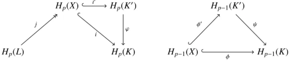
Proof. Let K0=K\stK . Let X be a solution to the dimension p reconstruction problem
of the pair (K, L). By Lemma9, we have L ✓ X ✓ K0. Consider the commutative
diagram of Figure8(left) where all maps are induced by inclusions. Since X is a p-Hp(X) Hp(K0) Hp(L) Hp(K) i0 i ' j Hp 1(K0) Hp 1(X) Hp 1(K) 0
Figure 8: Commutative diagrams for the proof of Lemma10. Left: injectivity of i implies injectivity of i0.
Right: injectivity of implies injectivity of 0.
reconstruction of the pair (K, L), i is injective and j is surjective. Since i = ' i0, the map
i0is also injective and thus im(i0 j) Hp(X), showing that X is also a p-reconstruction
of the pair (K0,L).
We now use the easiness of the pair (K, L) to prove the easiness of the pair (K0,L).
Consider an arbitrary simplicial complex X such that L ✓ X ✓ K0and the commutative
diagram of Figure8(right) where all maps are induced by inclusions. Since = 0,
the injectivity of implies the injectivity of 0. ⇤
Suppose (K, L) is an easily p-reconstructible pair. From Lemma10, it follows that at each step of the reconstruction algorithm, (K0,L) is also an easily p-reconstructible pair.
If Hp(K0) 6 im Hp(L ,! K0), we claim that we can always find a (K0,L)-homology
generating p-simplex . Indeed, by assumption, every p-simplex in K0\ L is positive
for every filtration F containing L and K0. This implies that @ is the boundary of
some p-chain c 2 Cp(L) for every p-simplex in K0\ L. The classes [ + c]K0, where
is a p-simplex in K0\ L, together with im Hp(L ,! K0), generate Hp(K0). Since
Hp(K0) 6 im Hp(L ,! K0), there must be a such that [ + c]K0 < im Hp(L ,! K0).
Both finding a c for a given and deciding whether [ + c]K02 im Hp(L ,! K0) can be
done in time polynomial in the size of K0.
The size of K0decreases strictly during the course of the algorithm. Since K is finite,
the algorithm has to stop eventually, and when it stops, we have Hp(K0) im Hp(L ,!
K0) im Hp(L ,! K).
In practice, we need not test whether or not the pair (K, L) satisfies the easiness property. It suffices to run the algorithm and check if the resulting complex K0 is
a p-reconstruction. If the pair (K, L) is not easily p-reconstructible (as in Figure1), the algorithm will output a simplicial complex X nested between L and K whose p-dimensional Betti number will di↵er from the persistent Betti number p(L ,! K).
Nonetheless, if (K, L) has any p-reconstruction, it must be a subset of K0, and the
algorithm may occasionally output a reconstruction even for pairs (K, L) that do not enjoy the easiness property.
5.2. Reconstruction in 3D
First, we review the use of persistent homology groups for homological inference, as proposed in [10,5]. Second, we formulate the problem of reconstructing a 3D shape as one of finding a subcomplex reconstruction of a simplicial pair which enjoys the property to be easily 1-reconstructible. Assuming a solution exists, we then describe how to build it in polynomial time. We use the notation ⌦↵={x 2 Rn: d(x, ⌦) ↵}.
Definition 6. Let ⌦ ⇢ Rnand let S ⇢ Rn be finite. We say that S is a homological
( , ✏)-sample of ⌦ if ⌦ ✓ S , S ✓ ⌦✏, and both
H⇤(⌦ ,! ⌦+✏) and H⇤(⌦+✏,! ⌦2 +2✏)
are isomorphisms.
Roughly, is a bound on the sampling density, and ✏ is a bound on the sampling error. If S is a homological ( , ✏)-sample of ⌦, then the plain arrows in the following diagram commute:
H⇤(⌦) H⇤(⌦+✏) H⇤(⌦2 +2✏)
H⇤(S ) H⇤(S2 +✏)
Moreover, the morphism im H⇤(⌦+✏,! S2 +✏) defines an isomorphism from H⇤(⌦+✏)
to im H⇤(S ,! S2 +✏). Hence, im H⇤(S ,! S2 +✏) H⇤(⌦).
Given as input a point set S that samples ⌦, we are thus able to infer the homology groups of ⌦ from S by computing the persistent homology groups of the pair (S2 +✏,S ).
Moreover we have the following lemma:
Lemma 11. Let S be a homological ( , ✏)-sample of ⌦ ⇢ Rn with ✏. Then
H0(S ,! S2 +✏) is an isomorphism.
Proof. First, note that H0(S ,! S2 +✏) is surjective, since every component of S2 +✏
contains a point of S ⇢ S . It remains to prove that H0(S ,! S2 +✏) is injective.
We first show that H0(⌦ ,! S ) is surjective. Let x 2 S . There is s 2 S with
d(x, s) . Moreover, there is y 2 ⌦ with d(s, y) ✏. Since ✏ , the two points x and y are both contained in the ball of radius around s and hence in the same connected component of S . In other words, every connected component of S contains a point of ⌦, so H0(⌦ ,! S ) is surjective.
Since H0(⌦ ,! ⌦+✏) is an isomorphism, this implies that H0(S ,! ⌦+✏) must
be injective. By injectivity of H0(⌦+✏ ,! S2 +✏), we obtain that H0(S ,! S2 +✏) is
injective. ⇤
In practice, we replace each S↵in the pair by the corresponding ↵-complex of S
which can be computed efficiently in R3using the Delaunay triangulation. We recall
that the Delaunay triangulation is the set of simplices ⇢ S for which there exists a ball whose boundary contains the vertices of and which encloses no point of S in its interior. Such a ball is said to be empty. The ↵-complex, denoted A↵(S ), is the
subcomplex of the Delaunay triangulation obtained by keeping simplices that fit in an empty ball of radius ↵ or less. It is a deformation retraction of the o↵set S↵.
We now focus our attention on the case n = 3 and ✏. It turns out that in this case we can find a subcomplex reconstruction of the pair of ↵-complexes (K, L) = (A2 +✏(S ), A (S )) in polynomial time, if one exists. Note that for each ↵ 0, the
o↵set S↵deformation retracts to A
↵(S ), and the pair (S2 +✏,S ) has a subspace
recon-struction ⌦+✏. Note however that this does not imply that (K, L) has a (subcomplex or
subspace) reconstruction. From now on, we assume that a subcomplex reconstruction of (K, L) exists. We next describe how to find one under this assumption.
Since H0(L ,! K) is an isomorphism by Lemma11and since there are no new
vertices in K \ L, this implies that every complex nested between L and K is a 0-reconstruction. Moreover, no edge in K \ L joins two connected components of L; in other words, (K, L) is easily 1-reconstructible. Construct a 1-reconstruction K0as
described above. Recall that this takes time polynomial in the size of K.
By Alexander duality, the finite connected components of the complement R3\ K0
correspond to classes in H2(K0). Hence, K00is a 2-reconstruction of (K0,L) if and only
if any two components of R3\ K0that lie in the same component of R3\ L are also
contained in the same component of R3\ K00(see Figure9for an analogous illustration
in R2). We note that such a 2-reconstruction of (K0,L) is also a 2-reconstruction of
(K, L) because H2(K0,! K) is injective as cavities in K0cannot be destroyed in K by
of dimension 2 and 3 from K0in order to connect all components in R3\ K0that are in
the same component of R3\ L.
Consider the dual graph G of K0, whose vertices are the tetrahedra of K0together
with the connected components of R3\ K0, and whose edges correspond to the triangles
of K0; see Figure9. Let G0be the subgraph of G whose edges correspond to triangles
in K0\ L. Now two components of R3\ K0lie in the same component of R3\ L if and
only if they are connected by a path in G0. Removing the corresponding triangles and
tetrahedra from K0merges the two components of the complement R3\ K0. Repeating
this procedure while there are mergeable components, we obtain a complex K00with
H2(K00) im H2(L ,! K). The construction of K00can also be done in polynomial
time.
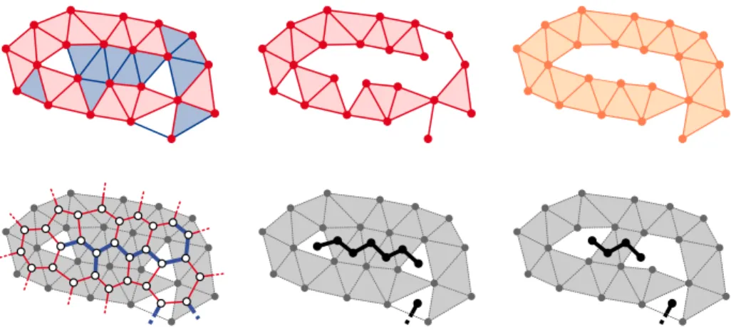
Figure 9: Top: A pair (K0,L) embedded in Rnand its (n 1)-reconstruction for n = 2. Bottom from left
to right: graph G whose edges correspond to (n 1)-simplices of K0and subgraph G0whose (bold) edges
correspond to (n 1)-simplices of K0\ L. Paths joining connected components of Rn\ K0in G0. Applying
simplicial collapses along a path to merge two connected components.
Note that this procedure will not a↵ect the property that the resulting complex K00
is a 1-reconstruction: two components in the complement of K0can be merged in the
complement of K00by a sequence of simplicial collapses on K0, followed by the removal
of a 2-simplex of K0with empty coboundary; see Figure9, bottom. This triangle must
be positive, since its removal merges two components of the complement. In other words, its removal will not destroy any 1-cycle in the 1-reconstruction. The resulting complex K00is thus a reconstruction of (K, L). We conclude:
Theorem 7. Let S be a homological ( , ✏)-sample of ⌦ ⇢ R3 with ✏. Then the
subcomplex reconstruction problem for the pair of ↵-complexes (A2 +✏(S ), A (S )) can
be solved in polynomial time. If a reconstruction exists, its homology is isomorphic to that of ⌦.
6. Conclusion
The homological reconstruction problem of simplicial pairs embedded in R3 is
in R3has a level set or a sublevel set reconstruction. We deduce that simplifying the
homology of a simplicial pair embedded in R3is also NP-hard and so is the homological
simplification of level and sublevel sets of real-valued simplexwise linear functions in R3. On the other hand, such problems can be solved in polynomial time if we
restrict ourselves to pairs of ↵-complexes in R3that admit homological inference of a
compact space, given an appropriate sample. Can we use this construction to devise a shape reconstruction algorithm with homological guarantees under the same sampling conditions?
Acknowledgements. This work was initiated during the 10thMcGill–INRIA Workshop
on Computational Geometry at the Bellairs Research Institute. The authors wish to thank all the participants for creating a pleasant and stimulating atmosphere, in particular Nina Amenta for discussions leading to a first version of Theorem1. Some of the authors were partially supported by the GIGA ANR grant (contract ANR-09-BLAN-0331-01), the European project CG-Learning (contract 255827), and the Toposys project FP7-ICT-318493-STREP.
[1] D. Attali and A. Lieutier. Optimal reconstruction might be hard. Discrete & Computational Geometry, 49(2):133–156, 2013.
[2] D. Attali, A. Lieutier, and D. Salinas. Vietoris–Rips complexes also provide
topologically correct reconstructions of sampled shapes. Computational Geometry,
46(4):448–465, 2013.
[3] P. Bendich, H. Edelsbrunner, D. Morozov, and A. Patel. Homology and robustness
of level and interlevel sets. Homology, Homotopy and Applications, 15(1):51–72,
2013.
[4] P. Bubenik and J. Scott. Categorification of persistent homology. Discrete & Computational Geometry, 2014. Available online.
[5] F. Chazal and A. Lieutier. Stability and computation of topological invariants of
solids in Rn. Discrete and Computational Geometry, 37(4):601–617, 2007.
[6] F. Chazal and A. Lieutier. Smooth manifold reconstruction from noisy and
non-uniform approximation with guarantees. Computational Geometry, 40(2):156–170,
2008.
[7] F. Chazal, D. Cohen-Steiner, and A. Lieutier.A sampling theory for compact sets
in Euclidean space. Discrete & Computational Geometry, 41(3):461–479, 2009.
[8] F. Chazal, V. de Silva, M. Glisse, and S. Oudot. The structure and stability of
persistence modules. Preprint, 2012. arXiv:1207.3674.
[9] D. Cohen-Steiner, H. Edelsbrunner, and D. Morozov. Vines and vineyards by
updating persistence in linear time. In Proceedings of the Twenty-second Annual
Symposium on Computational Geometry, SCG ’06, pages 119–126. ACM, 2006. [10] D. Cohen-Steiner, H. Edelsbrunner, and J. Harer.Stability of persistence diagrams.
[11] D. Cohen-Steiner, H. Edelsbrunner, and J. Harer. Extending persistence using
Poincaré and Lefschetz duality. Foundations of Computational Mathematics, 9(1):
79–103, 2008.
[12] V. de Silva and G. Carlsson.Topological estimation using witness complexes. In Eurographics Symposium on Point-Based Graphics, pages 157–166, 2004. [13] H. Edelsbrunner. Alpha shapes — a survey. In R. van de Weygaert, G. Vegter,
J. Ritzerveld, and V. Icke, editors, Tessellations in the Sciences: Virtues, Techniques and Applications of Geometric Tilings. Springer Verlag. To appear.
[14] H. Edelsbrunner and M. Kerber. Alexander duality for functions: the persistent
behavior of land and water and shore. In Proceedings of the 2012 symposium on
Computational Geometry, pages 249–258. ACM, 2012.
[15] H. Edelsbrunner, D. Letscher, and A. Zomorodian.Topological persistence and
simplification. Discrete & Computational Geometry, 28(4):511–533, 2002.
[16] H. Edelsbrunner, D. Morozov, and A. Patel.Quantifying transversality by
measur-ing the robustness of intersections. Foundations of Computational Mathematics,
11(3):345–361, 2011.
[17] A. Hatcher.Algebraic Topology. Cambridge University Press, 2002.
[18] W. Kühnel. Triangulations of manifolds with few vertices. In F. Tricerri, editor, Advances in di↵erential geometry and topology, pages 59–114. World Scientific, Singapore, 1990.
[19] N. Milosavljevi´c, D. Morozov, and P. Skraba.Zigzag persistent homology in matrix
multiplication time. In Proceedings of the twenty-seventh annual symposium on
Computational geometry, SoCG ’11, pages 216–225. ACM, 2011.
[20] D. Morozov.Homological Illusions of Persistence and Stability. PhD thesis, Duke University, 2008.
[21] P. Niyogi, S. Smale, and S. Weinberger.Finding the homology of submanifolds
with high confidence from random samples. Discrete & Computational Geometry,
39(1-3):419–441, 2008.