Control of Eukaryotic Cell Migration Through
Modulation of Extracellular Chemoattractant Gradients
The MIT Faculty has made this article openly available.
Please share
how this access benefits you. Your story matters.
Citation
Farahat, Waleed A., and H. Harry Asada. “Control of Eukaryotic Cell
Migration Through Modulation of Extracellular Chemoattractant
Gradients.” ASME 2010 Dynamic Systems and Control Conference,
Volume 1, 12-15 September, 2010, Cambridge, Massachusetts,
ASME, 2010, pp. 397–404. © 2010 by ASME
As Published
http://dx.doi.org/10.1115/DSCC2010-4190
Publisher
ASME International
Version
Final published version
Citable link
http://hdl.handle.net/1721.1/118767
Terms of Use
Article is made available in accordance with the publisher's
policy and may be subject to US copyright law. Please refer to the
publisher's site for terms of use.
CONTROL OF EUKARYOTIC CELL MIGRATION THROUGH MODULATION OF
EXTRACELLULAR CHEMOATTRACTANT GRADIENTS
Waleed A. Farahat
Department of Mechanical Engineering Massachusetts Institute of Technology
Cambridge, Massachusetts 02139 Email: wfarahat@mit.edu
H. Harry Asada
Department of Mechanical Engineering Massachusetts Institute of Technology
Cambridge, Massachusetts 02139 Email: asada@mit.edu
ABSTRACT
Cell migration is fundamental to a wide range of biological and physiological functions including: wound healing, immune defense, cancer metastasis, as well as the formation and devel-opment of biological structures such as vascular and neural net-works. In these diverse processes, cell migration is influenced by a broad set of external mechanical and biochemical cues, partic-ularly the presence of (time dependent) spatial gradients of solu-ble chemoattractants in the extracellular domain. Many biologi-cal models have been proposed to explain the mechanisms lead-ing to the migratory response of cells as a function of these ex-ternal cues. Based on such models, here we propose approaches to controlling the chemotactic response of eukaryotic cells by modulating their micro-environments in vitro (for example, us-ing a microfluidic chemotaxis chamber). By explicitly modelus-ing i) chemoattractant-receptor binding kinetics, ii) diffusion dynam-ics in the extracellular domain, and iii) the chemotactic response of cells, models for the migration processes arise. Based on those models, optimal control formulations are derived. We present simulation results, and suggest experimental approaches to con-trolling cellular motility in vitro, which can be used as a basis for cellular manipulation and control.
INTRODUCTION
Cell migration and motility is fundamental to many bio-logical and physiobio-logical processes. Simple bacteria, such as E. Coli, swim by adaptively modulating flagellar tumbling and turning rates. This enables swimming towards favorable envi-ronments, which leads to survival and prosperity of the bacterial and colony [1]. Complex eukaryotic cells migrate by constantly remodeling their cytoskeletons to achieve a wide arrange of key
biological functions. For example, in the context of structural development, endothelial tip cells guide the formation of vascu-lar sprouts achieve viable capilvascu-lary networks [2], whereas neural growth cones guide axonal migration that is necessary for form-ing neural interconnections [3]. In the context of wound healform-ing, epithelial cells migrate towards wound sites to build protective barriers, while neutrophils migrate to chase invading bacteria and microbes, eventually engulfing and digesting them in an impor-tant defense mechanism [4]. In the context of cancer metastasis, tumor cell migration is a necessary step for intravasation into the capillary vessels [5], eventually leading to its transport via blood into far reaching locations in the body. Common to all of these diverse examples is the premise that cells migrate in response to extracellular environmental cues. These cues can be either one or a combination of the following factors: i) the presence of gradients of soluble growth factors or chemoattractants that ini-tiate and guide cell movement along gradient directions, ii) the presence of insoluble molecules bound to the extra cellular ma-trix that also influence the cell’s trajectory, and iii) the presence of mechanical interactions between cells and their neighboring cells and extracellular matrix.
Here we study the problem of controlling cell migration by presenting external chemoattractant gradients as environmental cues. These gradients are established by modulating the bound-ary conditions of a diffusive extracellular region. Consequently, these boundary conditions become control inputs for affecting and guiding the migration process. Eukaryotic cells can sense very shallow gradients (as little as a 2% difference of growth fac-tor concentrations across the cell body). When presented with such a stimulus, cells respond through a complex sequence of signalling activity [6] by switching to a migratory phenotype, and commencing on a continual processes of remodelling their Proceedings of the ASME 2010 Dynamic Systems and Control Conference
DSCC2010 September 12-15, 2010, Cambridge, Massachusetts, USA
cytoskeletons via polymerization and disassembly of actin fil-aments [7]. Additionally, the placement and removal of focal adhesion points enable the cells to bind to the extra-cellular ma-trix, and consequently translocate their cell bodies towards the direction of movement [4]. When cells move in trajectories that are aligned with chemoattractant gradients, the process is known as chemotaxis. When cell trajectories are random, and are not directed along the gradients, the migration process is known as chemokinesis.
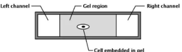
Because in vivo cell migration is influenced by a multitude of interacting factors, it is important to address the problem under simplified and well understood physical conditions. Therefore, studying migration under in vitro settings that precisely enable control of chemoattractant gradients is desirable. Microfluidic devices are currently being used to achieve this tasks for a va-riety of settings and cell cultures [8, 9]. While various forms of such devices exist, many consist of a gel region that acts as a surrogate to the extra-cellular matrix. Two channels run along the length of the gel region are used to flow media containing different concentrations of growth factors. Figure 1(a) shows the cross-section schematic of a representative device. The flow rate and composition of this media can be externally controlled via upstream mixers and instrumentation, thereby enabling the con-trol of the concentration of the media at the boundary of the re-gion. The growth factors defuse from the channels into the gel region, and present to the cells with time-varying growth factor concentrations and gradients. The growth factors bind to the re-ceptors differentially along the cell membrane, causing the cells to polarize and migrate. Because the growth factor concentra-tions are dynamic, they present the cell with gradients in space and time. These gradients induce cytoskeletal remodeling lead-ing to the mechanisms of cell migration. Therefore, to achieve a representative model of the process, diffusion dynamics, in ad-dition to chemoattractant-reception binding kinetics have to be modeled.
The framework described above provides an approach to controlling and manipulating cellular migration in vitro. For some problems, it may be desirable to maximize cell migration rates and distances, for example, in the case of maximizing an-giogenic sprouting response of endothelial monolayers. This can be cast as an optimal control problem that maximizes a distance traveled metric. In other conditions, it may be desirable to have the cells follow certain paths for patterning and structural forma-tion. This can be viewed as a trajectory control problem.
In this work, we model the problem setting described above, and derive optimal control formulations to guide cell migration. Our objective is to induce and control cellular motion within the gel region by dynamically altering the growth factor concentra-tions of the media flowing in the channels. In effect, this changes the boundary conditions on the gel region, and therefore the mi-croenvironment presented to the cells.
(a) Cross-section of a representative gel region (extra-cellular matrix) bounded by two channels.
(b) Diffusion region.
(c) Discretized region.
Figure 1. Problem setup. (a) The concentration profiles (c(y,t)) in the 1-dimensional diffusion model is controlled by the concentrations of the media in the left and right channels (uL anduR). (b) Discretization of the diffusion problem.
SYSTEM MODEL
We are concerned with the migration of a single cell in a purely diffusive, 1-dimensional homogeneous medium (varia-tions along channel length and height are ignored). The con-centration profile in the medium is determined entirely by diffu-sion, and the time-history of the concentrations of the media at the boundary of the region. Growth factors bind to cell mem-brane bound receptors, and a certain fraction of the receptors be-come occupied. Due to the presence of spatial gradients of the chemoattractants, a difference in the fraction of receptors occu-pied is established between the leading and trailing edges. This difference leads to cell polarization and the initiation of the mi-gratory signaling pathways. Therefore, there are three elements to the system model that are described below: i) diffusion dy-namics of the chemoattractants in the extra-cellular domain, ii) growth factor and receptor binding kinetics, and iii) model of cellular responses due the the difference in fraction of receptors occupied.
Diffusion dynamics
Diffusion in the medium is governed by the differential equation
∂c(y, t) ∂t = D
∂2c(y,t)
∂y2 + R(y,t) (1) where D is the diffusion coefficient (assumed constant through-out the entire region), and c(y,t) is the concentration of the growth factor in the medium at spatial coordinate y and time t. The spatial coordinate considered is one-dimensional and bounded, i.e. y ∈ [0,Y ], since minimal variance along the other channel dimensions. The boundary conditions of this region are c(0,t) = uL(t) and c(Y,t) = uR(t). R(y,t) is the reaction rate which can be used to model either growth factor sources (such as when tumors emit chemoattractants) or sinks (such as when cells internalize the chemoattractants). In our model, we assume that the amount of growth factor binding to the cells is negligible compared to the quantities existing in the medium, and therefore we assume R(y,t) = 0.
It is convenient to spatially discretize the gel region and write difference equations of the diffusion process. This allows for the diffusion dynamics to be written in an LTI form where the state of the diffusion subsystem is the vector of growth factor concentrations at the discretization grid points. Discretizing over a grid of N points, yi, with i ∈ [1, N], the difference approxima-tion of eq. (1) is given by:
∂c(yi,t) ∂t = D ∂2c(yi,t) ∂x2 ≈ D ci+1(t) − 2ci(t) + ci−1(t) (∆y)2 (2) ∂c(y1,t) ∂t ≈ D c2(t) − 2c1(t) + uL(t) (∆y)2 (3) ∂cN(yN,t) ∂t ≈ D uR(t) − 2cN(t) + cN−1(t) (∆y)2 (4)
where ∆y = N/Y is the grid spacing. Based on this difference approximation, the following state representation of the diffusion dynamics is written: ⎧ ⎨ ⎩ ˙ c1 ˙ c2 .. . ˙ cN ⎫ ⎬ ⎭ = D (∆y)2 ⎡ ⎢ ⎢ ⎢ ⎢ ⎢ ⎣ −2 1 1 −2 1 1 −2 1 . .. . .. . .. 1 −2 1 ⎤ ⎥ ⎥ ⎥ ⎥ ⎥ ⎦ ⎧ ⎨ ⎩ c1 c2 .. . cN ⎫ ⎬ ⎭ + D (∆y)2 ⎡ ⎢ ⎢ ⎢ ⎢ ⎢ ⎣ 1 0 0 0 .. . ... 0 1 ⎤ ⎥ ⎥ ⎥ ⎥ ⎥ ⎦ { uL uR } (5)
Equation (5) can be compactly written as
˙c = Acc + Bcuc (6) Receptor-growth factor binding kinetics
The kinetics of the growth factor (which is the ligand, L, in this case) and the membrane bound receptor (R), into a product (P) of an occupied receptor (as illustrated in fig. 2):
[L] + [R] ⇌ [P] (7)
The dynamics of this interaction are driven by the law of mass action, which can be written in differential equation form as fol-lows:
d[P]
dt = kon[L][R] − ko f f[P] (8) where konand ko f f are the forward and backward reaction rates respectively, and the notation [⋅] denotes the concentration of the argument. Assuming steady-state conditions of the binding ki-netics, the derivative terms vanish, leading to:
0 = kon[L][R] − ko f f[P] (9) [P] = 1
kD
[L][R] (10)
where kD = ko f f/kon is the reaction disassociation constant. The steady-state assumption is justifiable because the reaction binding kinetics of the growth factor and receptor typically reach steady state within a few micro-seconds for such proteins, whereas meaningful cellular migration time scales are typically on the order of hours.
The fraction of receptors occupied (FRO) in any region of the cell membrane is therefore given by
FRO = [P] [P] + [R] = [R][L]/kD [R][L]/kD+ [R] = [L] [L] + kD = c(y,t) c(y,t) + kD (11) where the last equality follows since c(y,t) is the concentration of the growth factor, or the ligand (L). The difference in fraction of receptors occupied between the leading and trailing edge of the cell. The location of the leading edge of the cell is given by y+ w, while the location of the trailing edge is given by y − w. Therefore, we write uδ(t) = c(y + w,t) c(y + w,t) + kD − c(y − w,t) c(y − w,t) + kD (12)
Figure 2. Illustration of ligand (red circles) binding to membrane bound receptors (blue) in the presence of a ligand concentration gradient. As a result, the fraction of receptors occupied on the right side is greater than the fraction of receptors occupied on the left side.
Since the concentrations at the leading and trailing edges of the cells depend on cell locations, means for interpolating the concentrations as a function of the concentrations at the grid point locations ciare necessary. We rely on Gaussian radial ba-sis functions to ensure smoothness of the interpolating functions (linear interpolations are necessarily discontinuous). Thus, the interpolated concentration for an arbitrary location y is given by
c(y,t) = N
∑
i=1 ci(t) ⋅ e −(yi−y σ )2 = cT(t) ⋅ d(ycell) (13)where yiis the grid coordinate, and σ is the spread of the Gaus-sian radial basis function, and the ith element of the vector d is e−
(yi−y
σ
)2 .
Cell migration model
To model the response of the cell as a function of the dif-ference in fraction of receptors occupied, we rely on a migration model presented in [10]. In this model, cell motion is driven by a random noise component, a chemotactic component, and an au-toregressive (damping-like) term. Modifying this model to our problem setting, and focusing on the deterministic aspects of the model, we write:
¨
ycell= −β ˙ycell+ κ ⋅ uδ (14)
where β is the autoregressive velocity term, and κ is known as the chemotactic responsiveness of the cell. While this model can be
viewed as highly simplistic, it has been shown to reproduce cell migration patterns in a qualitatively similar way to experimental observations [10].
Integrated System Model
To integrate equations (6), (12), and (14) into a common system model, it is useful to expand the input state vector to in-clude various intermediate variables as fictitious control inputs. We expand the control input vector, and write
u = ⎧ ⎨ ⎩ uL uR uδ uCL uCR ⎫ ⎬ ⎭ = ⎧ ⎨ ⎩ uL uR uδ c(ycell− w) c(ycell+ w) ⎫ ⎬ ⎭ (15)
where the definitions of the various quantities are self-evident. This allows us to write the dynamics of the system in the follow-ing LTI form:
⎧ ⎨ ⎩ ∣ ˙c ∣ ¨ ycell ˙ ycell ⎫ ⎬ ⎭ = ⎡ ⎢ ⎢ ⎢ ⎢ ⎢ ⎢ ⎢ ⎢ ⎣ .. . Ac 0 .. . −β 0 ⋅ ⋅ ⋅ 0 ⋅ ⋅ ⋅ 1 0 ⎤ ⎥ ⎥ ⎥ ⎥ ⎥ ⎥ ⎥ ⎥ ⎦ ⎧ ⎨ ⎩ ∣ c ∣ ˙ ycell ycell ⎫ ⎬ ⎭ + ⎡ ⎢ ⎢ ⎢ ⎢ ⎢ ⎢ ⎢ ⎢ ⎢ ⎣ D/(∆y)2 0 ... ... ... 0 ... 0 0 0 .. . ... ... ... D/(∆y)2 0 0 κ 0 0 0 0 0 0 0 ⎤ ⎥ ⎥ ⎥ ⎥ ⎥ ⎥ ⎥ ⎥ ⎥ ⎦ ⎧ ⎨ ⎩ uL uR uδ uCL uCR ⎫ ⎬ ⎭ (16)
Because the 5 × 1 input vector u has been expanded from the 2 × 1 vector uc, algebraic constraints relating the control inputs have to be satisfied. Specifically:
uδ= uCR uCR+ kD − uCL uCL+ kD (17) uCL= N
∑
i=1 ci⋅ e −(yi−(ycell −w)σ )2 = cT⋅ dL(ycell) (18) uCR= N∑
i=1 ci⋅ e −(yi−(ycell +w) σ )2 = cT⋅ dR(ycell) (19)In summary, equations (16) to (19) can be compactly written as
˙x = Ax + Bu (20)
s.t. g(x, u) = 0 (21)
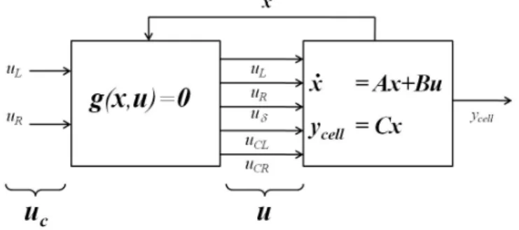
In this compact form, it becomes apparent that the model as-sumes a Hammerstein-like model structure as depicted in fig. 3.
Figure 3. A Hammerstein-like model representation of the cell migration process.
Open-loop Simulations
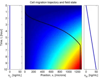
Open-loop simulations illustrating the system response are shown in Figure 4. The Figure shows the time evolution of the concentration gradients in the extracellular domain, and the re-sulting cell trajectories. Simulations are shown for different put concentrations at the left and right boundary channels, in-cluding: constant levels (4(a)), linear ramps (4(b)), sinusoidal (4(c)) and square inputs (4(d)). The values of the simulation pa-rameters were chosen to replicate the dynamics of the Vascular Endothelial Growth Factor (VEGF) diffusion through a medium of collagen, and the binding kinetics to the VEGF receptor on endothelial cells. These parameters are: D = 5 × 10⁻¹¹[m2/s], kD= 1 × 10⁻⁹[M] and cell dimensions of approximately 50 [mi-crons]. All simulations start at zero concentration levels in the extracellular domain, and with the cells adjacent to the left chan-nel.
The simulations suggest an interesting outcome: if maximal migration velocities are desired, extremal controls are not neces-sarily optimal. For example, in Figure 4(a), the chemoattractant concentration at the right channel was maintained at a maximal value of 50 ng/mL at all times, whereas the corresponding con-centration in Figure 4(b) was a linearly increasing ramp leading up to 50 ng/mL only after 10 hours. Even though the chemoat-tractant input in Figure 4(b) was less, the cells responded more rapidly by traveling across the domain in less time. This perhaps counter-intuitive result motivates the need to cast the migration control problem in an optimal control framework, which is dis-cussed next.
AN OPTIMAL CONTROL FORMULATION
We propose an optimal control formulation relying on the Pontryagin Minimum Principle [11] to enable cell trajectory con-trol as it migrates through the diffusion medium. The cost func-tion formulafunc-tion is given by:
u∗= arg min u { ϕ(x∣t=T) + ∫T 0
L
(x, u)dt } (22). We chose a general Lagrangian cost function is given by
L
=α 2(ycell− ydes) 2+γ 2(u 2 L+ u2R) + υ (23)and the terminal cost that maximizes net cell migration
ϕ(x∣t=T) = −ycell= −xN+2 (24)
This cost function can be specialized to various cases via appro-priate parameter settings. For example, in most practical cases, there is no cost associated with the control inputs uLand uRsince they represent chemoattractant concentrations. This can be cap-tured by setting γ = 0. Similarly, if cell trajectory following is desired, we set all coefficients other than α to zero. If minimum travel time from extremal points is desired, we set all coefficients other than υ to zero.
We define the Hamiltonian scalar function
H
asH
= λTf(x, u) +L
(x, u) + µTg(x, u) (25) where the (N + 2) × 1 co-states vector λ includes the Lagrange multipliers associated with the dynamic constraint (20) and the 3 × 1 vector µ = [µδ, µCL, µCR]T includes the Lagrange multipliers associated with the algebraic input control constraints (17), (18), and (19).From the Pontryagin Minimum Principle, the optimal con-trol and optimal trajectories are characterized by:
˙ λ ∗ = −∇x
H
(26) u∗= arg min u {H
} (27)where (⋅)∗ denotes quantity optimality. Equation (26) can be used to characterize the optimal co-states trajectories λ∗(t). Equation 27, is used the define the optimal controls. In most cases it can be equivalently characterized by ∇u
H
= 0, thereby defining 5 constraints. Two of these constraints are used to de-fine the real control inputs (uL, uR), while the remaining three constraints define the multipliers (µδ, µCL, µCR). The first two re-lations define the optimal control inputs as follows:(a) Zero input at left channel, constant input at right channel. (b) Zero input at left channel, linear input at right channel.
(c) Sinusoidal input at both channels. (d) Zero input at left channel, Square input at right channel.
Figure 4. Simulation results showing the input concentrations at the left channel, right channel, and the time evolution of the field concentration long time. The location of the cell is initiated at the left end of the field. The cell trajectory is illustrated by the black line. (a) Constant concentrations applied (Ul= 0anduR= 50for all time). (b) Linearly ramping concentrations in the right channels. (c) Sinusoidal concentrations on both channels. (d) Pulsatile concentrations on the right channel.
∂
H
∂uL = D (∆y)2λ1+ γuL ⇒ u∗L= ⎧ ⎨ ⎩ uLmax if − λ1 γ D (∆y)2 > uLmax −λ1 γ D (∆y)2 if uLmin< − λ1 γ D (∆y)2 < uLmax uLmin if − λ1 γ D (∆y)2 < uLmin (28) and ∂H
∂uR = D (∆y)2λN+ γuR ⇒ u∗R= ⎧ ⎨ ⎩ uRmax if − λN γ D (∆y)2 > uRmax −λ1 γ D (∆y)2 if uRmin< − λN γ D (∆y)2 < uRmax uRmin if − λN γ D (∆y)2 < uRmin (29)Note that in cases when γ = 0, optimal controls u∗L and u∗R take the form of bang-bang control. This is primarily due to the
Hamiltonian not being a function of the inputs. The remaining three relations define the multipliers µ as follows:
∂
H
∂uδ = λN+1κ +∂L
∂uδ + µδ ⇒ µ∗δ= −λN+1κ (30) ∂H
∂uCL = ∂L
∂uCL + µδ kD (uCL+ kD)2 + µCL ⇒ µCL∗ = λN+1κkD (uCL+ kD)2 (31) ∂H
∂uCR = ∂L
∂uCR − µδ kD (uCR+ kD)2+ µCR ⇒ µ∗CR= − λN+1κkD (uCR+ kD)2 (32)Finally, the optimal costate trajectories are given by:
˙ λ∗= −ATλ − ∇x
L
− µCL { ∇xdL⋅ c +[ d0L ]} − µCR { ∇xdR⋅ c +[ d0R ]} (33) where∇x
L
= [0, ⋅ ⋅ ⋅ , 0, α(ycell− ydes)]TThus, to solve for the optimal controls, state trajectories, co-state trajectories and Lagrange multipliers, equations (28) - (33) have to be solved simultaneously. The boundary conditions of the solutions are given by
x(t = 0) = 0 (34)
λ(t = T ) = ∇x⋅ ϕ(t = T )
= [0, 0, ⋅ ⋅ ⋅ , 0, −1] (35) These equations and the boundary conditions characterize the optimal trajectories.
CONCLUSIONS
We presented a model and an approach to the problem of controlling cell migration. A key feature of eukaryotic cell mi-gration is that mimi-gration velocities depend on the difference of
fraction of receptors occupied. A simple growth factor-receptor binding kinetics model reveals that the inputs are transformed nonlinearly to what is otherwise assumed to an LTI process. We developed a Hammerstein-like model of this process. Simula-tions showed that in order to maximize cell migration rates across a region, extremal controls are not necessarily optimal. This mo-tivated the derivation of optimal control conditions by relying on the Pontryagin minimum principle.
ACKNOWLEDGEMENTS
This work is funded by the Singapore-MIT Alliance for Re-search and Technology (SMART - BioSym IRG) and the Na-tional Science Foundation - Emerging Frontiers in Research and Innovation (NSF-EFRI) program (grant #0735997).
REFERENCES
[1] Alon, U., Surette, M. G., Barkai, N., and Leibler, S., 1998. “Robustness in bacterial chemotaxis”. Nature, 397, pp. 168–171.
[2] Barkefors, I., Le Jan, S., Jakobsson, L., Hejll, E., Carlson, G., Johansson, H., Jarvius, J., Park, J. W., Li Jeon, N., and Kreuger, J., 2008. “Endothelial Cell Migration in Stable Gradients of Vascular Endothelial Growth Factor A and Fi-broblast Growth Factor 2”. Journal of Biological Chem-istry,283(20), pp. 13905–13912.
[3] Huber, A. B., Kolodkin, A. L., Ginty, D. D., and Cloutier, J.-F., 2003. “Signaling at the growth cone: Ligand-receptor complexes and the control of axon growth and guidance”. Annual Review of Neuroscience,26(1), pp. 509–563. [4] Lodish, H., Berk, A., Kaiser, C., Krieger, M., Scott, M.,
Bretscher, A., Ploegh, H., and Matsudaira, P., 2008. Molec-ular Cell Biology, sixth ed. W. H. Freeman and Company. [5] Folkman, J., 2007. “Angiogenesis: an organizing principle
for drug discovery?s”. Nature Reviews, 6, pp. 273–286. [6] Levchenko, A., and Iglesias, P. A., 2002. “Models of
eu-karyotic gradient sensing: Application to chemotaxis of amoebae and neutrophils”. Biophysical Journal, 82(1), pp. 50 – 63.
[7] Pollard, T. D., and Borisy, G. G., 2003. “Cellular motil-ity driven by assembly and disassembly of actin filaments”. Cell,112(4), pp. 453 – 465.
[8] Chung, S., R.Sudo, P. J. Mack, P., Wan, C., Vickerman, V., and Kamm, R. D., 2009. “Cell migration into scaffolds un-der co-culture conditions in a microfluidic platform.”. Lab Chip,9, pp. 269–275.
[9] Wang, S.-J., Saadi, W., Lin, F., Nguyen, C. M.-C., and Jeon, N. L., 2004. “Differential effects of egf gradient profiles on mda-mb-231 breast cancer cell chemotaxis”. Experimental Cell Research,300(1), pp. 180 – 189.
[10] Stokes, C., Lauffenburger, D., and Williams, S., 1991. “Mi-gration of individual microvessel endothelial cells:
stochas-tic model and parameter measurement”. J Cell Sci, 99(2), pp. 419–430.
[11] Bryson, A. E., and Ho, Y.-C., 1975. Applied Optimal Con-trol: Optimization, Estimation and Control. John Wiley & Sons, New York.