MASSACHUSETTS INSTITUTE OF TECHNOLOGY ARTIFICIAL INTELLIGENCE LABORATORY
Working Paper No. 332 December 1990
Correction of Force Errors for Flexible
Manipulators in Quasi-Static Conditions
Antonio Bicchi
Claudio Melchiorri
Abstract
This paper deals with the problem of controlling the interactions of flexible manipulators with their environment. For executing a force control task, a manipulator with intrinsic (mechanical) compliance has some advantages over the rigid manipulators commonly employed in position control tasks. In particular, stability margins of the force control loop are increased, and robustness to uncertainties in the model of the environment is improved for compliant arms. On the other hand, the deformations of the arm under the applied load give rise to errors, that ultimately reflect in force control errors. This paper addresses the problem of evaluating these errors, and of compensating for them with suitable joint angle corrections. A solution to this problem is proposed in the simplifying assumptions that an accurate model of the arm flexibility is known, and that quasi-static corrections are of interest.
Copyright @ Massachusetts Institute of Technology, 1990
A. 1. Laboratory Working Papers are produced for internal circulation, and may
con-tain information that is, for example, too preliminary or too detailed for formal publication. It is not intended that they should be considered papers to which reference can be made in the literature.
1
Introduction
When a manipulator interacts with the environment, there is a force exchange between the links of the robot and the object(s) being contacted. In many robotics applications, the assigned task consists in precisely applying a specified force and/or moment to the environ-ment (force control problem); in addition, the control of motions of the robot end-effector
along some directions can be specified (hybrid control problem). In order to accomplish such tasks, it is necessary to achieve a precise positioning of the part(s) of the manipulator in contact with the environment. On the other hand, force control of manipulators poses diffi-cult problems, as abundantly illustrated in literature (a classical review is given by Whitney [1987]). Probably, the most important of these problems is the tendency of force control loops to become unstable in presence of small perturbations of the model parameters used to design the controller. One of the reasons of this difficulty can be described very loosely by noting that the control of the contact forces between two objects within a given accuracy is equivalent to controlling their relative position within an accuracy k times higher, where k here is the combined stiffness of the bodies, and is typically a very large number. Reducing the stiffness of the robot-environment system is therefore a viable way of alleviating force control problems: a more precise formulation of this concept can be found e.g. in [Roberts, Paul, and Hillberry, 1985], [Eppinger and Seering, 1987], and [Chiou and Shahinpoor, 1990]. This observation suggests an interesting application of flexible robots, that might encour-age to design future robots with a built-in compliance. Besides this advantencour-age, the design of lightweight, slender link robot arms meets other important requirements in applications such as space or underwater, and could reduce the cost of robot arms.
However, if the manipulator is composed of flexible links, and/or its joints are compliant, the positioning accuracy of the robot may be greatly reduced. Neglecting its flexibility, i.e. considering the manipulator as a chain of rigid bodies connected by perfect joints, the arm position in the world frame can be evaluated on the basis of the joint positions and the forward kinematic equations. This estimate of the arm posture is usually very inaccurate for flexible manipulators in contact with the environment, due to the deformation of its structure caused by contact forces.
In order to reduce these positioning errors, the force information provided by the force sensors used to close the force control loop can be exploited. However, these sensors are usually located as close as possible to the end-effector, so that the measured force is expressed in a reference frame whose position and orientation in the world frame depend in turn on the elastic deformations. A consequence is that the force information provided by the sensors cannot be directly used in the control loop. However, if a model of the arm compliance is available, it is possible, by means of a recursive algorithm, to compute that position and orientation. We will describe and use such an algorithm in section 4 to evaluate the real position and orientation of a flexible robot given the forces acting on it. A substantially equivalent method for predicting the deflection of serial manipulators with flexible links and
joints has been presented by Fresonke, Hernandez, and Tesar [1988].
Once the deflections of the arm under the given load are known, appropriate corrections of the robot inputs can be applied to minimize the force/position errors due to flexibility. Since the overall deflection of the robot is comprised of both joint and link flexibilities, the determination of this correction is not trivial.
In this paper, we will be mostly concerned with the problem of finding the optimal joint position in order to minimize the error in a force-control task. This problem is basically regarded as a planning phase preceding real-time implementation, so that a quasi-static assumption is made, and dynamic effects of flexibility are disregarded. In general, the modification that may be applied to the joint inputs will be able to compensate only in part for the deformation of the manipulator. On the other hand, the case when there are more joints than strictly necessary in the kinematic chain (redundant manipulators) is also considered. In order to homogeneously treat both such defective and redundant cases, the correction problem is cast in a nonlinear optimization framework, as described in section 3. The paper is organized as follows. In section 2, the model considered for the links of the flexible manipulator is described, and the main assumptions used in this paper are given. In section 3 the problem of the force error compensation is formulated as a minimization problem, and an algorithm for its solution is presented. Section 4 describes some specific details of the algorithm in the context under consideration, while section 5 reports some examples. The final section 6 concludes with comments about the suggested technique and plans for future activity.
2
Model of the Flexible Arm
In this section, both a general description of the problem, considering a flexible robot arm in interaction with an environment that reacts to its movements, and the simplifying
assump-tions used in the rest of the paper are presented.
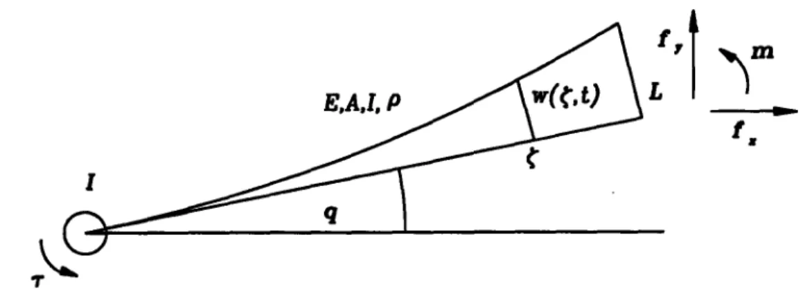
The general structure of a flexible arm dynamics can be described by a set of partial differential equations, of degree two for the torsional and axial modes, and four for the bending modes of the links. Consider for instance the simple manipulator link depicted in Figure 1, with constant cross-section and lying in a horizontal plane. In this case, only the axial and bending deflections of the link in the plane are of interest. The axial dynamics can be written as
02 02x
EA d - d- = O (1)
where C is the coordinate along the undeformed beam axis, x = x((, t) is the displacement
at time t of the section initially in (, E is the elastic modulus of the link, and p its mass per unit length.
A
rmf
'N
IL
Figure 1: A simple manipulator link and its elastic model The bending dynamics of the flexible link can be written as
a
4y
2y
EJ- + p•- = 0 (2)
where J is the cross-sectional moment of inertia of the beam, and y is defined as (see e.g. [Korolov and Chen, 1988])
y(C, t) = w(C, t) + (q.
Here, w is the elastic displacement measured from the undeformed axis (see Figure 1), and q is the nominal (hub) position of the joint. Note that lumped joint elasticity is not considered in this example.
The overall manipulator dynamic relationship can be built (for serial link arms) by con-catenating differential equations of this type by their boundary conditions, that express the equilibrium of control torques, inertial moments, and constraints at the ends of the links. In the example of Figure 1, boundary conditions for eq. (1) can be written as
EA,] C=L f, (3)
x(0,t) = 0, (4)
where A is the cross-section area, L is the total length of the link, and f, is the axial component of the force exerted on the link's end by the hub of the next link (or by the environment if the distal link of the arm is considered). The four boundary conditions for eq. (2) are:
EJ i9j=oJ+ T - = 0; (5) y(0,t) = 0; (6) EJ a(2 m; (7) C=L EJ 0(3 fy, (8) C=L
where r is the control torque on the joint preceding the link under consideration, Jh the lumped moment of inertia at the hub, f, and m the bending component of the force and the torque applied at the link's extremity.
The force f and torque m at the link end balance nex t link's forces and control torque, except for the distal link, for which they represent the environment reaction on the robot end-effector. These interaction forces, in general both time and space-varying, act as a forcing input on the dynamic chain.
When only quasi-static conditions are considered, dynamic terms in the relationships above can be neglected. Therefore, eq. (1) and eq. (2) reduce to the following ordinary differential equations of elastic beams:
82xS- 0,
(9) a(2
4y
- 0. (10)
Deflections of links under the loads applied at their extremities can be determined by integrating such relationships. For instance, integrating eq. (9) with the boundary conditions
( 3), ( 4), we obtain:
LfA
EA'
while integration of eq. (10) with the boundary conditions ( 6)-( 8) leads to:
L3f, L2m Ay = + 3EJ 2EJ' T2f Tm 2EJ LEJ = E E "I
where Ax, Ay are the displacements of the extremity of the link along the link axis and normal to it, respectively, and AO is the rotation of the link's end.
In the three-dimensional case, similar relationships hold, and a general linear equation relating the six elastic displacements of the link's end with the applied load can be written in matrix form as:
0 L3 0 0 0 L2 3EJ 2EJ EJ 0 2EJ 0 0 0 0 0 0 0 S 0 0 0 0 -0 0 0 0 0 L L2 2EJ Ej L
I]m
(11)
where Ad and AO are the displacements and rotation vectors of the link's extremity in 3D space, G is the shear modulus of the link's material, and Jo is the polar momentum of the beam cross section.
The forces and torques on the distal ends of the links can be evaluated by means of static equilibrium considerations, using the recursive algorithm presented in section 4. The recursive calculation is started at the last link, where the load coincides with the robot
-environment interaction forces, which are assumed to be known (by means e.g. of a wrist mounted force/torque sensor). However, this knowledge is relative to a reference frame E fixed to the end-effector. By solving the elastic displacements of every link, the geometric re-lationship of the end-effector frame E with the fixed (base) frame B can be found. Therefore,
also the relationship between the interaction forces in E and in B is established as
mf BRE 0 Ef
Bf P[ RE BRE Em (12)
where Bpe is a skew-symmetric matrix equivalent to the cross product (Bp x), being Bp
the vector of the linear displacements of the end-effector caused by both the flexibility and the kinematics of the mechanism, and BRE is the corresponding rotation matrix.
Introducing the symbol BKE for the force tranformation matrix, and the vector w =
[fT mT]T (wrench), we rewrite for convenience eq. (12) as
BW = BKE EW (13)
3
Compensation of Force Errors
In general, the wrench computed in eq. (13) is not equal to the desired one. It is therefore required to take some corrective actions, i.e. to apply proper set-points to the position/force controllers of the manipulator joints in order to compensate for the error.
The correction of interaction force errors may be cast in a nonlinear optimization problem form. The kernel of the adopted algorithm may be related to the steepest descent method [Press et al., 1986], and it has been utilized in other fields of robotics, in particular in the solution of the inverse kinematic problem for redundant and non-redundant manipulators, see for instance [Balestrino, DeMaria and Sciavicco, 1984], [Wolovich and Elliott, 1984],
[Sciavicco and Siciliano, 1986, 1988], [Das, Slotine and Sheridan, 1988]. The basic idea is the following. Define a wrench error as
Bed
]
r:--
B BBw
e = B= Bw
-and a quadratic positive definite function as
eTPe
V(e) 2 (14)
where P is a symmetric positive definite matrix. Because of equations (12)-(13), the wrench Bw is a function of q, so that V(e) depends on the joint position vector. The optimal joint positions q are those minimizing V(q), and therefore we seek a control law for the arm joint positions such that the robot is driven towards the optimal configuration. Since V(q) may be regarded as a Lyapunov function, the convergence to its minimum is guaranteed if the position control law is such that the value of V is kept decreasing along the trajectories of the system.
In the continuous time domain, the convergence to the minimum is achieved if the fol-lowing Lyapunov condition is satisfied:
S= eTPe < 0. (15) Since e = Bwd - B BWd - BKE EW it follows that S d O(BKE Ew)
at
S a q q
W
IKw (a)
Figure 2: Block diagram of the proposed algorithm. or
e = B - G4 (16)
being G = 8(BK" 1w) the Jacobian matrix of Bw. If the update law f or the joint position is chosen as
4 = A + [ ]GPe, A > 0, (17)
(e PGGTPe)
it can be easily shown that the condition (15) is verified.
Sciavicco and Siciliano [1988], using the same algorithm for solving the inverse kinematic problem, pointed out how eq. (17) may be, for computational convenience, simplified to
1 = "AGT Pe,
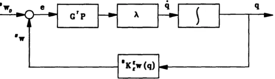
allowing in this case the function V to be negative-definite only outside a region of the error space containing the stability point e = 0. In this way, the maximum tracking error is directly related to xd and inversely to A, while in steady state, since id = 0, the tracking error will be in any case zero. In this situation, an increase in the gain A results into a reduction of the tracking error, which may therefore be arbitrarily reduced. The resulting algorithm is shown in the form of a block diagram in Figure 2.
In discrete time, the stability proof of the algorithm is more complex. A detailed discus-sion of such proof has been presented in [Das, Slotine, and Sheridan, 1988] for the inverse kinematic solution of redundant manipulators. One of the major modifications in the dis-crete time version of the algorithm is that, in order both to obtain the maximum convergence rate for the scheme and to avoid instability problems, the gain A has to be updated at each
sampling period T. In fact, given the discrete time version of the Lyapunov function, eq. (14), at t = nT
e Pen
V, 2
the goal is now to make negative the difference V,+1 - Vn. If the joint velocities are computed
at the instant t = nT as
4n = AnGPen,
the convergence of the algorithm is guaranteed with the choice
1 e(PTGSG T Pen
T e(PTGnSnG7PGnSGPen
where Sn is a diagonal matrix whose elements are properly computed to limit the maximum values of GT P en, [Das, Slotine, and Sheridan, 1988].
A final observation relative to this scheme concerns the possibility of getting "stuck", i.e. to generate a null joint velocity vector, 4 = 0, also if e : 0. This happens when Pe E Null(GT). However, this does not represent a serious limitation to the applica-bility of the algorithm. As a matter of fact, besides being an easily detectable condition
(4 = 0; e : 0), it can be argued that the term Pe can be easily modified in such a way that
Pe 0 Null(GT). This is performed by adding suitable constraints on the joint space (as done by Das, Slotine and Sheridan [1988]), or in the task space (as suggested by Sciavicco and Siciliano [1986]). Obviously, in this latter case if the trajectory has some components which are constantly in Null(GT), no algorithm will be able to compensate for tracking errors.
4
Computation of the Matrices
BKEand G
In order to apply the algorithm, it is necessary to compute the matrices BKE and G
-8(BKE EW)
8q , eq. (13), eq. (16). In this section, these two matrices are calculated for a manipulator with a generic kinematic structure with n degree-of-freedom.
4.1 Computation of the force/torque transform matrix BKE In the previous sections, the wrench error has been defined as
where the wrench transformation matrix, see eq. (12), is defined as
[
BRE 0 (18)BKE = B RE B (18)
The sub-matrices BRE and Bp® are in general complex functions of the compliance of the
joints, of the link flexibility and of the kinematics of the manipulator. Since these quantities depend on the interaction forces and the joint position, in general it is not trivial to compute the matrix BKE. A possible and efficient way to determine this matrix is to use a recursive method, consisting in computing the effects of the force/torque applied to the i-th link on the (i-1)-th link, starting with the distal link. These effects are expressed by a transformation matrix Ki, with the same structure of the transformation matrix in eq. (18), and such that
wi-1 = Kiwi (19)
Therefore, the matrix EKE can be expressed as the product of the Ki as
BKE = K1K2... K.= 'iKi (20)
i=1
where the generic term Ki, according to the hypothesis of small deformations, can be com-puted as
Ki = Ki,ki.(qi)Kioint(ri)Ki,f•le (wi) (21)
where Ki,kin depends on the geometry of the link, Kiiot on the joint compliance, and Ki,ft•e,, on the link flexibility. In the following, the expressions of these three transformation matri-ces are given. For the sake of simplicity, in the following discussion only rotational joints are taken into account in the kinematic structure of the manipulator: however, equivalent considerations may be done also for the case of prismatic joints.
The elements of the matrices Ri,kin and P®,i,kin are only functions of the geometric and kinematic parameters of the i-th link. Using. the Denavit-Hartenberger notation, qi- 1 is the nominal joint angle, ai and di are the twist and the offset of the i-th link, and ai represents the length of the link. The expressions of the matrices Ri,kin and P®,i,kin are
Ri,kn = Sqi-_lo, Cq,_l 8 Cj -- S, (22)
and
0 -cadi aisq,_1 - Cq,_iS8,di
Pikin - Cidi 0 -aicqi_1 - Sqgi_l•idi (23)
-- ais_ + cqi.S, d; aicq,i_ + Sqi_ Saidi 0
where 8, = sin(x) and c, = cos(x), as usual in transform matrices.
The matrix Kijoit is composed by the sub-matrices Ri,oint and P®,ijoint
cC -s' 0
Riioint = Rot(zi, kcini) = s c' ' 0
001 and
0 0 ai sin(k,,iri)
Pe,ijoit = 0 0 ai[1 - cos(kc,iri)]
-ai sin(kc,ir) -ai[1 - cos(kc,ii)] 0
where ke,i and ri are the joint compliance and the torque acting on the joint, respectively. Finally, the i-th matrix Ki,flex is composed by the submatrices Ri,-lez and P®,i,fle,, whose elements are functions of the elastic displacements of the link. The evaluation of such displacements is not an easy task in general. Some sophisticated techniques, such as finite elements methods, can be applied profitably to this problem; in other cases, a direcxt
calibration of displacements under known loads can be a viable solution to obtain a flexibility model for the arm. For our purposes here, however, a rather simple flexibility model for the links, considered as slender beams with constant section, can suffice. In the hypothesis of small elastic deformations, the linear and rotational displacements of the link, expressed as a 6-dimensional vector, are as shown in section 2, eq. (11):
[
di,zfle• AOfidlex 0 0 0 0 0 0 0 0 0 0 0 0 -" 3EJ 0 -_- 2EJ 0 0 0 0 a 0 0 a2. 2EJ EJ 0 ~- 0 0 0 ai 2EJ EJThe matrix Ri,fl, is computed as a rotation matrix about an axis parallel to 60i,fp,e of an angle given by the module of 6Oi,fle,. As pointed out in [Fresonke, Hernandez and Tesar,
1988], this approximation is valid as long as small deformations are assumed.
The recursive computation of eq. (19), starting from the distal joint for which the force/torque sensor provides Ew, yields the deformations generated by the flexibility and the joint compliance, and therefore all the matrices in eq. (20), allowing the transformation of the force vector from the frame E located in the end-effector to the base frame B .
4.2
Computation of the Jacobian Matrix G =
B--The application of the algorithm presented in section 3 requires the computation of the matrix G = = -- K•q;w), in which, in general, both BKE and Ew are functions of the joint position vector q. Since the wrench transformation matrix EKE is a function of the joint positions, see equations (12), (13), the Jacobian matrix G may be computed as
8(BKE EW) O(ln=1 K, EW)
G-aq 8q
O(fI=1K,) Ew n aEw
O(rfl 1 K,) Ew + n .Ow
=-w
Oq+ (it
i=1 xK,)
OIn general, the computation of this matrix requires the knowledge of the manipulator-environment interaction, eq. (11), for the calculation of . In following, only the case in
which Ew may be considered constant in the range of motion caused by elastic displacements is taken into account. The matrix G may be computed as
G • (l 1Ki) EW T EW
aq
where T is a three-dimensional matrix composed by n Ti (6x6) matrices given by Ti = (IT=(Ti
J7
I Kj,kinKj~jo•.Kj,f•) K d OKj,kin3 ,kinKjitiK 1,f.,) -K-,kqi ( Ki,jointKj,flezKj+l,kin)
j=1 dl j=i
where conventionally we assume Kn+l,kin = 16. Therefore, the generic i-th column of the matrix G is calculated as
5
Case Studies
In this section, two examples of the application of the algorithm to the force control of flexible manipulators in interaction with the environment are illustrated. One of the characteristics of the presented technique is that the algorithm allows consideration of robots with arbitrary number of degrees of freedom (both redundant and defective), as well as with arbitrary link shape. Note that in eq. (22), (23) the complete set of Denavit-Hartenberg parameters are taken into account.
The case studies address the simulation of two planar manipulators with rotational joints. The manipulators are a planar 3 degree-of-freedom and a redundant 5 degree-of-freedom planar arm. All the links of both manipulators are assumed to have the same geometrical and mechanical structure, with a circular cross-section with radius 10 mm, and a length of 1000 mm. The material elastic constants are those of common steel, while for the joints a compliance of kd = 10' (Nm/rad) has been assumed. The matri x P is, in both the examples, an identity matrix with proper dimensional units. Finally, in both the cases, the presented algorithm is iterated until a value V(e) < 10'- for the error function is reached.
5.1
A 3 Degree-of-Freedom Planar Manipulator
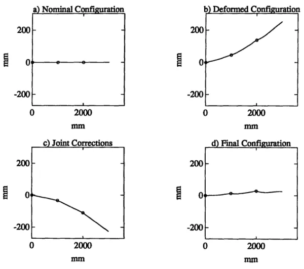
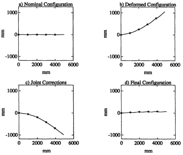
The manipulator considered in the first example consists of three links and three rotational joints with parallel axes. A wrench Ew = 0 10 0 0 0 0 0] (N)-(Nm) is supposed to be applied at the tip of the arm. The initial - undeformed - pose of the manipulator is shown in Figure 3.a. The effects of the applied wrench on the compliant structure are
reported in Figure 3.b, where the deformed configuration of the manipulator is shown. It has to be pointed out that, since the joint encoiders are placed before the elastic elements, the arm appears to the control system to be in the undeformed configuration reported in Figure 3.a. In this situation, if the force set-point Bwd = [ 0 10 0 0 0 30 ]T (N)-(Nm) is specified, a force error Be = 11.1561 0.067 0 0 0 0.02506 T (N)-(Nm) results. In
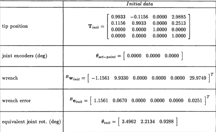
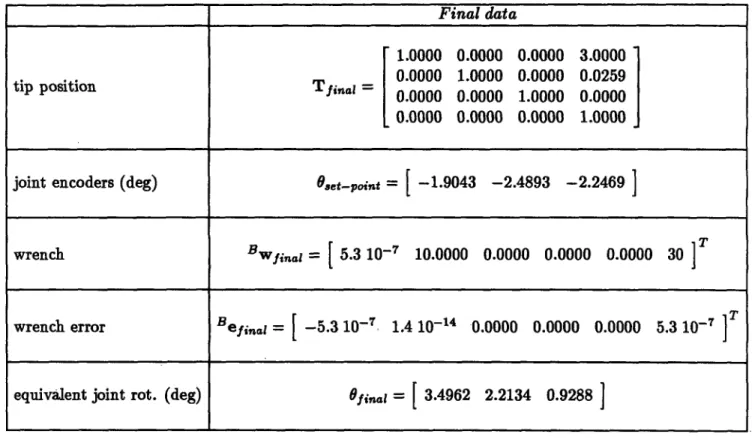
Figure 3.c the computed corrective actions on the joint positions are shown, i.e. the nominal configuration to which the arm joints have to be positioned to minimize the force error e. In Figure 3.d the final (compensated) configuration of the arm is shown. In Table 1.a,b nu-merical results relative to this case are presented. In particular, Table 1.a reports the initial position/orientation, the measurements of the joint encoders, the initial applied wrench ex-pressed in the base frame, the wrench error and the initial -virtual -joint rotation equivalent to the rotation/flexion of the structure. In Table 1.b the relative data after the correction are reported. The final value of the error function is V(e) < 10- 6, and this result is achieved in 335 steps.
b) Deformed Confieuration 200 0 -200 2000 mm 2000 mm c) Joint Corrections 01 -200 2000 d) Final Configuration 2000 mm
Figure 3: The four configurations ot the the three-link arm discussed in section 5.1. 0 -200 -0---- -__
I
17
200 &O -200 a) Nominal Configuration ) 0t--~c~-tip position
joint encoders (deg)
wrench
wrench error
equivalent joint rot. (deg)
Initial data 0.9933 -0.1156 0.0000 2.9885 0.1156 0.9933 0.0000 0.2513 init -0.0000 0.0000 1.0000 0.0000 0.0000 0.0000 0.0000 1.0000 Oset-point =
[
0.0000 0.0000 0.0000] Bwin, = -1.1561 9.9330 0.0000 0.0000 0.0000 29.9749 Beinit = 1.1561 0.0670 0.0000 0.0000 0.0000 0.0251 Oinit =[3.4962
2.2134 0.9288]tip position
joint encoders (deg)
wrench
wrench error
equivalent joint rot. (deg)
Final data 1.0000 0.0000 0.0000 3.0000 0.0000 1.0000 0.0000 0.0259 Tfinal = 0.0000 0.0000 1.0000 0.0000 0.0000 0.0000 0.0000 1.0000 O.e.toi. = [-1.9043 -2.4893 -2.2469] Bwfinal = [5.3 10- ' 10.0000 0.0000 0.0000 0.0000 30 ]T Befinl = -5.3 10-7 1.4 10 -14 0.0000 0.0000 0.0000 5.3 10- 7 Ofin.l= [3.4962 2.2134 0.9288
]
Table 1.b: The final configuration data for example 1.
5.2
A 5 Degree-of-Freedom Planar Redundant Manipulator
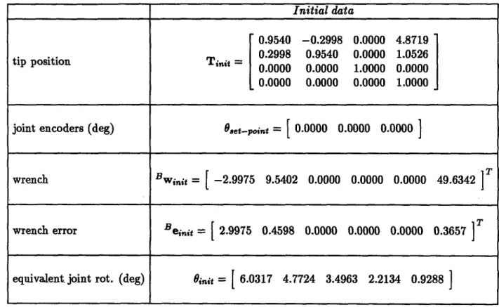
The second manipulator taken into consideration is a redundant planar arm. The robot, shown in Figure 4.a, is a 5 degree-of-freedom robot. A wrench Ew = [ 0 10 0 0 0 0 ]T (N)-(Nm) is supposed applied to the tip of the arm, as in the previuos case. In this case, the force error, with a set point Bwd = [ 0 10 0 0 0 50 ]' (N)-(Nm), is Be =
S2.29975
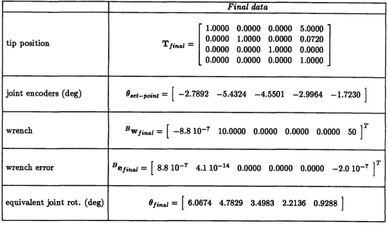
0.4598 0 0 0 0.3656 AT (N)-(Nm). In Figure 4.a-d the initial undeformed and deformed configurations, as well as t e corrective actions and the final position of the manip-ulator are shown. The numerical results relative to this example are reported in Table 2.a,b. In this case, because of the larger number of joints and the greater value of the initial error, a value of the error function V(e) = 9.110-6 is reached after 1427 iterations of the algorithm.1000 -1000 0 2000 4000 6000 b) Deformed Configuration ()] 2000 4000 6000 Inm c) Joint Corrections 1000 -1000 0 2000 4000 6000 d) Final Configuration 0 2000 4000 6000 mm mm
Figure 4: The four configurations ot the the three-link arm discussed in section 5.2.
1000 01 -1000 I I 1000 0 -1000 p p , a I I ! | 51\ hTnminsll rnrrfia~l+~~nn - v.--- vy. - - , --04
tip position
joint encoders (deg)
wrench
wrench error
equivalent. joint rot. (deg)
Initial data 0.9540 -0.2998 0.0000 4.8719 0.2998 0.9540 0.0000 1.0526 0.0000 0.0000 1.0000 0.0000 0.0000 0.0000 0.0000 1.0000 0.,et-oint =
[
0.0000 0.0000 0.0000]
Bin =[
-2.9975 9.5402 0.0000 0.0000 0.0000 49.6342]
Beinit= 2.9975 0.4598 0.0000 0.0000 0.0000 0.3657 Oinit=[
6.0317 4.7724 3.4963 2.2134 0.9288]
Table 2.a: The initial configuration data for example 2.
---tip position
joint encoders (deg)
wrench
wrench error
equivalent joint rot. (deg)
Final data 1.0000 0.0000 0.0000 5.0000 0.0000 1.0000 0.0000 0.0720 Tinl = 0.0000 0.0000 1.0000 0.0000 0.0000 0.0000 0.0000 1.0000 Oe-oit =
[
-2.7892 -5.4324 -4.5501 -2.9964 -1.7230 Bwfina = [-8.8 10- 7 10.0000 0.0000 0.0000 0.0000 50]
efinl =[
8.8 10- 7 4.1 10-1 4 0.0000 0.0000 0.0000 -2.0 10- ]T Ofi,•• = [6.0674 4.7829 3.4983 2.2136 0.9288 ]Table 2.a: The final configuration data for example 2.
6
Conclusions
In this paper, an algorithm for the compensation of interaction force errors for flexible manipulators has been presented. Because of joint compliance and link flexibility, the prob-lem is non-linear; the proposed solution employs the framework of non-linear optimization techniques. In fact, the presented algorithm is related to the steepest descent method, a well-known technique in this area. The method is also similar to algorithms proposed for the kinematic solution of redundant manipulators. The basic idea is to control joint positions so as to minimize a quadratic function force errors. A Lyapunov stability analysis demon-strates the stability and convergence of the method. Examples of the proposed algorithm are reported, showing the effectiveness of the technique also for the case of redundant arms. The proposed solution is used in this paper as an off-line reference generator.
Further developments of this research will investigate extensions of the method to more general problems. In particular, activity is currently in progress in the following areas:
* Modification of the method to take into account interaction forces that vary (in the end-effector reference frame) during the execution of the task, such as e.g. gravity and inertial loading;
* Modification of the iterative algorithm in order to achieve better convergence speed and trajectory smoothness, so as to allow the application of the method as an on-line (real-time) high-level force controller for flexible manipulators.
Acknowledgements
The authors wish to thank Dr. J. Kenneth Salisbury for the stimulating discussions. Support for this research is provided by the University Research Initiative Program under Office Naval Research Contract N00014-86-K-0685. Support for both the authors as Visiting Scientists at the A.I. Lab. has been provided by a NATO-CNR joint fellowship program, grants No. 215.22/07 and No. 215.23/15.
References
Balestrino, A., De Maria, G., Sciavicco, L., "Robust Control of Robotic Manipulators", Proc. 9th. IFAC World Congress, Budapest, Hungary, 1984.
Chiou, B.C., and Shahinpoor, M, "Stability Considerations for a two Link Force Con-trolled Flexible Manipulator", Proc. IEEE Int. Conf. on Robotics and Automation, May 1990.
Das, H., Slotine, J-J.E., Sheridan, T.B., "Inverse Kinematic Algorithms for Redundant Systems", Proc. IEEE Int. Conf. on Robotics and Automation, San Francisco, CA, 1988.
Eppinger, S.D., and Seering, W.P., "Understanding Bandwidth Limitations in Robot Force Control", Proc. IEEE Int. Conf. on Robotics and Automation, March 1987. Fresonke, D.A., Hernandez, E., Tesar, D., "Deflection Prediction for Serial Manipula-tor", Proc. IEEE Int. Conf. on Robotics and Automation, 1988.
Korolov, V.V., and Chen, Y.H.: "Robust Control of a Flexible Manipulator Arm", Proc. IEEE Conf. Robotics and Automation, Philadelphia, PA, 1988.
Press, W.H., Flannery, B.P., Teukolsky, S.A., Vetterling, W.T., "Numerical Recipes: The Art of Scientific Computing", Cambridge University Press, 1986.
Roberts, R.K., Paul, R.P., and Hillberry, B.M., "The Effect of Wrist Sensor Stiffness on the Control of Robot Manipulators", Proc IEEE Int. Conf. on Robotics and Automation, March 1985.
Sciavicco, L., Siciliano, B., "Coordinate Transformation: A Solution Algorithm for One Class of Robots", IEEE Trans. Syst., Man, Cybern., Vol. SMC-16, No. 4, July/Aug. 1986.
Sciavicco, L., Siciliano, B., "A Solution Algorithm to the Inverse Kinematic Problem for Redundant Manipulator", IEEE Jour. of Robotics and Automation, VoL 4, No. 4, Aug. 1988.
Whitney, D.E., "Historical Prespective and State of the Art in Robot Force Control", Int. Jour. of Robotic Research, Vol. 6, No. 1, Spring 1987.
Wolovich, W.A., Elliott, H., "A Computational Technique for Inverse Kinematics", Proc. 23rd. Conf. on Decision and Control, Las Vegas, NV, Dec. 1984.