HAL Id: hal-01636028
https://hal.archives-ouvertes.fr/hal-01636028
Submitted on 16 Nov 2017
HAL is a multi-disciplinary open access
archive for the deposit and dissemination of
sci-entific research documents, whether they are
pub-lished or not. The documents may come from
teaching and research institutions in France or
abroad, or from public or private research centers.
L’archive ouverte pluridisciplinaire HAL, est
destinée au dépôt et à la diffusion de documents
scientifiques de niveau recherche, publiés ou non,
émanant des établissements d’enseignement et de
recherche français ou étrangers, des laboratoires
publics ou privés.
Split energy cascade in turbulent thin fluid layers
Stefano Musacchio, Guido Boffetta
To cite this version:
Stefano Musacchio, Guido Boffetta. Split energy cascade in turbulent thin fluid layers. Physics of
Fluids, American Institute of Physics, 2017. �hal-01636028�
Stefano Musacchio
Universit´e Cˆote d’Azur, CNRS, LJAD, Nice, France
Guido Boffetta
Dipartimento di Fisica and INFN, Universit`a di Torino, via P. Giuria 1, 10125 Torino, Italy We discuss the phenomenology of the split energy cascade in a three-dimensional thin fluid layer by mean of high resolution numerical simulations of the Navier-Stokes equations. We observe the presence of both an inverse energy cascade at large scales, as predicted for two-dimensional turbu-lence, and of a direct energy cascade at small scales, as in three-dimensional turbulence. The inverse energy cascade is associated with a direct cascade of enstrophy in the intermediate range of scales. Notably, we find that the inverse cascade of energy in this system is not a pure 2D phenomenon, as the coupling with the 3D velocity field is necessary to guarantee the constancy of fluxes.
I. INTRODUCTION
Fifty years ago, Kraichnan showed in the seminal pa-per [1] that the dynamics of an incompressible flow in two-dimensions (2D) is dramatically different from the classical phenomenology of three-dimensional (3D) tur-bulence. The presence of two inviscid quadratic invari-ants, energy and enstrophy, gives rise to a double-cascade scenario [2]. At variance with the 3D case, in which the kinetic energy cascades toward small viscous scales, in 2D it is transferred toward large scales. Such “inverse energy cascade” is accompanied by a “direct enstrophy cascade”, which proceeds towards small scales [3]. In the inverse and direct ranges of scales the theory predicts a kinetic energy spectrum E(k) ≃ ε2f/3k−5/3 and E(k) ≃ η
2/3 f k−3
with possible logarithmic corrections [4]. Here and in the following εf and ηf denote the energy and the
enstro-phy injection rates respectively. The Kraichnan seminal concept of inverse cascade has become since then a pro-totypical model for several turbulent systems, from the inverse cascade in strongly rotating 3D flows [5], to the inverse cascade of magnetic helicity in three-dimensional magneto-hydrodynamic turbulence [6], of passive scalar in compressible turbulence [7], of wave action in weak turbulence [8].
The presence of the two cascades in two-dimensional turbulence has been observed in a number of numerical simulations [9–18] and in experiments in soap films [19– 25] and in thin fluid layers [26–28].
At variance with the numerical investigations, which allows to to study the ideal 2D Navier-Stokes equations, the experiments have to deal with the effects of the finite thickness of the fluid layer. This issue, which has been often considered a limitation for two-dimensional experi-ments, opens a series of interesting questions. How is the ideal 2D phenomenology modified in the case of a thin (3D) fluid layer? How thin should the layer be, in or-der to display the 2D-like double cascade? In which way does the transition from the 2D to the 3D regime occur at increasing the thickness of the layer?
These questions have been addressed both in numer-ical simulations [29, 30] and experiments [31, 32] which
have shown that the critical parameter which controls the cascade direction is the ratio S = Lz/Lf of the thickness
to the forcing scale. When S ≥ 1 the flow is 3D at the forcing scale and the injected energy produces a direct cascade as in usual 3D turbulence. By decreasing S one observes the phenomenon of cascade splitting with a frac-tion of the injected energy which goes to large scales and the remaining energy which flows to small scales [29, 30]. For S ≪ 1 the flux of the direct energy cascade is ex-pected to scale as S2
. This prediction has been verified in shell models for quasi-two-dimensional turbulence [33]. Further reducing S, the cascade of energy towards small scale vanishes when the thickness Lz reaches the
Kol-mogorov scale Lν and the flow recovers the standard 2D
phenomenology.
In the present paper we investigate the entanglement of 2D and 3D dynamics which occurs in a turbulent fluid layer by means of numerical simulations of the 3D Navier-Stokes equations in a confined domain with Lz < Lf
(and Lz > Lν). In agreement with previous findings,
we observe the phenomenon of splitting of the energy cascade. By introducing a suitable decomposition of the velocity field, we show that the inverse cascade involves mainly the kinetic energy of the 2D modes, while the energy of the remnant 3D velocity is transferred toward the viscous scales. We also show that the development of the inverse energy cascade is associated with a partial conservation of the enstrophy in the intermediate range of scales Lz< ℓ < Lf. Interestingly, we find that 3D modes
play a relevant role in the the 2D phenomenology which is observed at large scales. In particular, the transport of the 2D modes by the 3D velocity is necessary to ensure a constant flux of energy in the inverse cascade as well as a constant flux of enstrophy in the range Lz< ℓ < Lf.
The remaining of the paper is organized as follows. Section II introduces the Navier-Stokes equations and the decomposition of the velocity field in the 2D and 3D modes. In Section III we report the results of the numerical simulations. Section IV is devoted to the con-clusions. In the Appendix A we derive a 2D model for the dynamics of a thin layer in the limit Lz→ 0.
2
II. NAVIER-STOKES EQUATIONS FOR A THIN LAYER
We consider the dynamics of a three-dimensional thin layer of fluid, ruled by the Navier-Stokes equations for the velocity field u(x, t):
∂tu+ u · ∇u = −∇p + ν∆u + f (1)
where ν is the kinematic viscosity, f is the external forc-ing, and the pressure p is determined by the incompress-ibility constraint ∇·u = 0. The flow is confined in a thin domain of size Lx= Ly = rLz with r ≫ 1 and periodic
boundary conditions in all the directions.
In absence of forcing and dissipation, (1) preserves the kinetic energy E = (1/2)h|u|2
i (where h...i denotes aver-age over the space). The energy balance in the forced-dissipated case reads:
dE
dt = εf− εν (2) where εν = νh(∇u)2i is the energy dissipation rate due
to the viscosity and εf = hf · ui is the energy input
provided by the external forcing.
The forcing provides also an input of enstrophy Z = (1/2)h|ω|2
i, (ω = ∇ × u denotes the vorticity field) at the rate ηf = h(∇×f)·ωi. At variance with the ideal 2D
case, the enstrophy is not preserved by the full 3D invis-cid dynamics, but it is produced by the vortex stretching mechanism [34]. The equation for the vorticity field is obtained by taking the curl of (1)
∂tω+ u · ∇ω = ω · ∇u + ν∆ω + fω (3)
where fω = ∇ × f and ω · ∇u represents the vortex
stretching term.
In order to highlight the presence of a 2D phenomenol-ogy in the 3D flow, it is useful to decompose the ve-locity field as u = u2D + u3D . The 2D mode u2D = (u2D x (x, y), u 2D
y (x, y), 0) is defined as the average along
the z direction of the x and y components of the velocity field u, and it satisfies the 2D incompressibility condi-tion ∂xu2xD + ∂yu2yD = 0. In the Fourier space it
cor-responds to the mode k3 = 0 of the horizontal velocity
u2D
(k1, k2) = (ux(k1, k2), uy(k1, k2), 0). The field u 3D
is defined as the difference u3D = u − u2D. By the above
definitions it is easy to show that the total energy decom-poses into a 2D contribution E2D= (1/2)h|u2D|2
i and a 3D contribution E3D= (1/2)h|u3D|2
i as E = E2D+E3D.
We notice that, beside the kinetic energy of the verti-cal velocity, E3D contains also the contributions of the
modes k36= 0 of the horizontal components of the
veloc-ity.
Similarly, the vorticity field can be decomposed as ω = ω2Dzˆ+ ω3D, where ω2D = ∂
xu2yD− ∂yu2xD is the
scalar vorticity of the two-dimensional flow. In the limit of vanishing thickness Lz → 0 (at finite viscosity ν) the
vertical dependence disappears and u2D becomes
solu-tion of the 2D Navier-Stokes equasolu-tion (see Appendix A).
Therefore, it is reasonable to assume that the occurrence of an inverse energy cascade at finite thickness Lzshould
be associated to the dynamics of the 2D mode u2D.
III. DIRECT NUMERICAL SIMULATIONS
We performed a direct numerical simulation of the Navier-Stokes equations (1) in a confined geometry with periodic boundary conditions. The computational do-main has dimensions Lx = Ly = 2π, Lz = Lx/64
(r = 64) and it is discretized on a uniform grid at reso-lution Nx× Ny× Nz= 4096 × 4096 × 64. The numerical
simulations are performed by means of a fully-parallel, pseudospectral code, with 2/3 dealiasing scheme. We adopt an hyperviscous damping scheme (−1)p−1ν
p∆p
with p = 4 and νp= 10−21. We do not use any large-scale
dissipation (such as linear friction).
The flow is sustained by a “components, two-dimensional” forcing, that is, the forcing is active on the horizontal components of the velocity and it is dependent on the horizontal coordinates only, f = (fx(x, y), fy(x, y), 0). Therefore in the vorticity equation
(3) forcing fω is active on the 2D field ω2D only.
Forc-ing is restricted to a narrow wavenumber shell in Fourier space with kh= (k12+ k
2 2)
1/2
≃ kf, k3= 0. Here kf = 16.
The forcing is Gaussian and δ-correlated in time to con-trol the injection rates εf and ηf. The characteristic time
at the forcing scale is defined as τf = ηf−1/3. The ratio
between the thickness Lz = 2π/kz and the forcing scale
Lf = 2π/kf is S = Lz/Lf = 4 This ensures the regime
of split cascade with the coexistence of the 3D and the 2D phenomenology (see Fig. 1) [30].
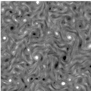
FIG. 1. Snapshot of the scalar vorticity field ω2D in the late stage of the simulation. Typical two-dimensional objects, such as strong vortices at the forcing scale Lf, coexist with small scale three-dimensional features.
0 10 20 30 40 0 20 40 60 80 100 0 1 2 3 4 E 2D / εf τf E 3D / εf τf t/τf
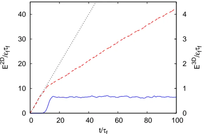
FIG. 2. Temporal evolution of the kinetic energy E2D (red, dashed line, left y-axis) and E3D (blue, solid line, right y-axis). The dotted line represents the linear growth with the input rate εf (left y-axis).
The velocity field at time t = 0 is initialized to zero, plus a small random perturbation, which is required to trigger the 3D instability. The results shown in this Sec-tion has been obtained with an energy of the initial per-turbation Epert ≃ 1.6 · 10−7εfτf.
Because of the purely 2D forcing, in the early stage of the simulation (t < 10τf), the energy accumulates in
the 2D mode u2D
at a rate equal to the forcing input, while the energy E3D of the 3D component is
negligi-ble (see Figure 2). The activation of the 3D modes u3D
(at t ≃ 10τf) is accompanied by a significant reduction
of the growth rate of the 2D energy as some of the in-jected energy is now transferred to small scales. At later times, E3D
saturates to a statistically steady value (as in standard 3D turbulence), while the two-dimensional component E2D energy keeps increasing with a constant
reduced rate εα < εf. We stop the simulation at time
t = 100τf, when the inverse energy cascade has reached
the lowest wavenumber (see Figure 4). Continuing the simulation for further times, in absence of large-scale dissipation, we expect that the kinetic energy will ac-cumulate in the lowest mode, giving rise to the so called “condensate” [35–37]. The 2D mode contains almost all the kinetic energy of the horizontal velocities, and the kinetic energy of the vertical component uz contained in
the mode k3= 0 represents only 24% of the total.
The enstrophy of the 2D mode Z2D = 1/2h(ω2D)2
i grows initially with the input rate ηf, reflecting the pure
2D nature of the initial flow (see Figure 3). As 3D mo-tions develop (at t ≃ 10τf), the enstrophy associated to
the 3D modes Z3D= 1/2h|ω3D|2
i increases very rapidly and reaches a stationary value which is much larger than the saturation level of Z2D.
0 5 10 15 20 25 0 20 40 60 80 100 0 50 100 150 200 250 Z 2D / ηf τf Z 3D / ηf τf t/τf
FIG. 3. Temporal evolution of the enstrophy of ω2D (red, dashed line, left y-axis) and ω3D (blue, solid line, right y-axis). The dotted line represents the linear growth with the input rate ηf (left y-axis).
A. Energy spectra 10-10 10-8 10-6 10-4 10-2 100 100 101 102 103 kf kz k-5/3 a b c d e f g E(k) k 10-10 10-8 10-6 10-4 10-2 100 100 101 102 103 kf kz k-5/3 a b c d e f g E(k) k
FIG. 4. Energy spectra E(k, t) at times t/τf = 4.6 (a, violet), 6.9 (b, green), 9.2 (c, cyan), 13.7 (d, orange), 18.3 (e, yellow), 45.8 (f, blue), 91.6 (g, red). The last three spectra are almost superposed for k > kz.
In Figure 4 we show the instantaneous spectra E(k, t) of the total energy at different times t. The initial spectra are almost completely 2D, because the forcing is active only on 2D modes. We observe that the 3D instability begins at high harmonics of the thickness wavenumber kz,
then it propagates to all the modes k > kz. The energy
spectrum at k > kf saturates at time t ≃ 16τf. At scales
larger than the forcing scale, k < kf, we observe the
development of an inverse energy cascade with a power-law spectrum E(k) ≃ ε2α/3k−5/3.
The “spiky” aspect of the energy spectrum at high wavenumbers k > kz is due to the anisotropic spacing of
4
the wavenumbers in the Fourier space. The separation between the discrete wavenumbers in the horizontal di-rection is ∆kh= 2π/Lxwhile in the vertical direction it is
∆k3= 2π/Lz= kz. Given that Lz≪ Lx, the
wavenum-ber space is structured as horizontal dense layers, sep-arated by large gaps in the vertical direction. Because the complete energy spectrum is defined as the integral of the square amplitude of the modes over a spherical wavenumber shell of radius k, one gets a sudden increase of the spectrum each time the spherical shell is a multiple of kz.
In order to analyze the contribution of the 2D mode to the total energy spectrum, it is interesting also to con-sider the 2D spectra E2D(k), in which the integral is
restricted to the horizontal wavenumbers kh=pk12+ k 2 2
on the plane k3= 0. In physical space, this is equivalent
of averaging first the velocity fields in the vertical direc-tion z and then computing the spectrum of the averaged 2D fields. It is worth to notice that, for k < kz, the 2D
spectra and 3D spectra coincide, because the spherical shell of radius k < kz intersects the planes k3 = ±mkz
only for m = 0. 10-8 10-6 10-4 10-2 100 100 101 102 103 kf kz k-5/3 k-5/3 E(k) k 10-8 10-6 10-4 10-2 100 100 101 102 103 kf kz k-5/3 k-5/3 E(k) k
FIG. 5. Energy spectrum E2D(k) of the 2D mode u2D (red, dashed line) and 3D mode u3D(blue, solid line). We also show the 2D spectrum of the vertically-averaged vertical velocity uz (black, dotted line). The spectra are computed at t = 100τf
In Figure 5 we compare the 2D energy spectrum E2D
(k) of the 2D mode u2D
with the 3D energy spectrum of the 3D mode u3D. At low wavenumbers k < k
zalmost
all the kinetic energy is contained in the 2D mode. This confirms that the inverse cascade which develops in the range k < kf concerns only the 2D energy. Conversely,
the 3D mode contains the largest fraction of the kinetic energy at high wavenumbers k > kz. Interestingly, in the
same range of wavenumber, the 2D spectrum of the 2D mode displays a −5/3 slope, and it is very close to the 2D spectrum of the vertical component uz.
The spectrum E2D(k) shown in Fig. 5 is reminescent of
the horizontal spectrum (of meridional and zonal winds) observed in the upper troposphere by the Global
Atmo-spheric Sampling Program [38] where a transition from a k−3 to a k−5/3 spectrum at small scales is observed.
We remark that, despite the similarities between the two spectra, the physical mechanisms are probably different (see, for example, [39], [40]) as the transition in the atmo-spheric spectrum is observed at a scale around 500 km, while in our simulations it occours at a scale comparable with tickness of the layer.
B. Spectral fluxes -1 -0.5 0 0.5 1 10-1 100 101 kz/kf ΠE (k)/ εf k/kf
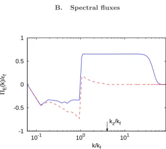
FIG. 6. Spectral energy flux ΠE(k) (blue solid line) and 2D energy flux (red, dashed line), at t = 100τf
The analysis of the spectral flux of the total kinetic en-ergy ΠE(k) shows that in a thin fluid layer the energy
in-jected by the forcing at the wavenumber kf indeed splits
in two parts (see Figure 6). At low wavenumbers k < kf
we observe a constant, negative flux of energy, which in-dicates the presence of an inverse energy transfer toward large scales. At high wavenumbers k > kfwe also observe
a constant energy flux, now positive, indicating a direct cascade of energy toward small scales. It is worth to re-mind that the kinetic energy transported in the direct cascade is not only that of the vertical component of the velocity, but contains also the contributions of the modes k36= 0 of the horizontal velocities. In this range of scales
the dynamics in the vertical and horizontal directions is strongly coupled, and the positive energy flux cannot be explained in terms of a direct cascade of the vertical ve-locity passively transported by a two-dimensional, three components (2D3C) flow [41–43].
As we have shown in Fig. 4, the inverse cascade in-volves mainly the energy of the 2D mode. This observa-tion suggests to check whether or not this inverse cascade coincides with a pure 2D dynamics of the 2D mode u2D.
To this purpose we have taken the fields u2D
and we have truncated them at kh= kzby setting to zero all the
modes with kh > kz. Then, we have computed the 2D
they were solutions of the two-dimensional Navier-Stokes equations. Surprisingly, we find that the 2D energy flux in the range of scales of the inverse cascade does not co-incide with the 3D flux shown in Fig. 5. The physical interpretation of this result is that the energy of the 2D mode is not simply transported toward large scales by the 2D flow itself, but the 3D modes contribute to the transport process. This contrasts with a 2D3C scenario at large scales, with the vertical velocity being passively transported by the 2D flow [41–43].
10-1 100 101 102 103 10-1 100 101 kf/kz ΠZ / ηf ΣZ / ηf k/kz
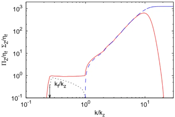
FIG. 7. Spectral enstrophy flux ΠZ(k) (red solid line), Spec-tral enstrophy production ΣZ(k) (blue, dashed line), and 2D enstrophy flux (black, dotted line), at t = 100τf
As discussed in Section II, the main difference between 3D and 2D Navier-Stokes equations is the absence of the vortex stretching term ω ·∇u in the latter. The presence of two positive-defined inviscid invariants (energy and en-strophy) causes the reversal of the direction of the energy cascade. Even if the enstrophy is not conserved by the 3D dynamics, it is tempting to conjecture that the devel-opment of the inverse cascade in thin fluid layers is due to a dynamical suppression of the enstrophy production. To investigate this issue we computed the total spectral enstrophy flux Πz(k) and the total spectral enstrophy
production ΣZ(k) defined as:
ΠZ = Z |q|≤kdq(v · ∇ω)(q)ω ∗(q) , (4) ΣZ= Z |q|≤kdq(ω · ∇v)(q)ω ∗(q) . (5)
In the range of wavenumbers kf < k < kz the
pro-duction of enstrophy is negligible, and the enstrophy flux is constant, as shown in Fig. 7. This constant flux cor-responds to the presence of a direct enstrophy cascade. At high wavenumbers, k > kz, the enstrophy production
becomes significant and therefore the enstrophy flux is not constant anymore but grows following the produc-tion term. Our results show that, in analogy with the case of ideal 2D Navier-Stokes equations, also in a thin fluid layer the emergence of the inverse energy cascade
is due to the presence of a “quasi invariant”, the en-strophy, which is conserved by the large-scale dynamics. Nonetheless, it is worth to notice, that the conservation of the enstrophy is not due to the transport by the 2D mode itself. Following the same procedure described in the case of the energy flux, we have computed the 2D enstrophy flux from the truncated 2D velocity fields. In the range of scale kf < k < kzthe 2D flux is positive, but
not constant, thus indicating that the full 3D dynamics is required for the conservation of enstrophy (see Fig. 7). The presence of an intermediate direct enstrophy cas-cade in the range of scales Lz< ℓ < Lf allows to derive a
simple dimensional argument for the scaling of the energy flux toward small scales. A direct cascade with constant enstrophy flux ηf = εfk2f carries also a residual energy
flux, which decreases as Π(k) ∼ εf(kf/k)2. By assuming
that the flux of energy of the direct cascade which starts from kz is equal to the residual flux Π(kz) carried by the
enstropy cascade at the scale kz, one gets the prediction
εν = Π(kz) ∼ εfS2. This prediction has been verified in
shell models for quasi-two-dimensional turbulence [33].
IV. CONCLUSIONS
In this paper we present a numerical study of the phe-nomenology of a turbulent flow confined in a thin fluid layer. We discuss the possibility to disentangle the com-plex mixture of 2D and 3D dynamics by a suitable de-composition of the velocity field in 2D and 3D modes.
In analogy with previous studies [29, 30], when the flow is forced at scales Lf larger that the thickness Lzof
the layer we observe a splitting of the energy cascade in two directions. A fraction of the energy is transported toward large scale, giving rise to an inverse energy cas-cade, while the remnant energy is transported toward the small viscous scales, as in 3D turbulence. We show that the inverse energy cascade is accompanied by the development of a direct cascade of enstrophy in the in-termediate range of scales Lz < ℓ < Lf. The enstrophy
production becomes relevant only at small scales ℓ < Lz,
allowing for a partial conservation of the enstrophy by the large-scale dynamics.
The scenario which emerges from our findings is a co-existence of 2D phenomenology, with a double cascade of energy and enstrophy `a la Kraichnan at large scales ℓ > Lz and a 3D direct energy cascade `a la Kolmogorov
at small scales ℓ < Lz. Interestingly, the decomposition
of the velocity field in the 2D modes and the remaining 3D part reveals that the 2D and 3D dynamics are deeply entangled. On one hand, we find that the energy and en-strophy which are involved in the double cascade at large scales are those of the 2D modes. On the other hand, the 3D velocity is necessary to guarantee a constant flux of 2D energy and enstrophy in the large-scale transport.
We plan to extend the analysis of the interactions be-tween 2D and 3D modes to the case of rotating and sta-bly stratified thin fluid layers. Previous results [44] shows
6
that rotation causes a suppression of the enstrophy pro-duction similar to the effects of confinement, favoring the two-dimensionalization of the flow and the development of the inverse energy cascade. Nonetheless, this effect is not accompanied by the presence of a range of scales in which the enstrophy is conserved by the large-scale dy-namics. This is likely to affect the interactions between 2D and 3D modes. In the case of stably stratified fluid layers, it has been shown that the conversion of kinetic energy into potential energy, which is promptly trans-ferred toward the small diffusive scales, provides a fast dissipative mechanism which suppresses the large scale energy transfer [45]. Investigating the interactions be-tween 2D vortical modes and 3D potential modes will improve the understanding of this process.
ACKNOWLEDGMENTS
Simulations have been performed at the Juelich Forschungszentrum (Germany) within the PRACE Prepatory project PRPA22 and at CSC (Finland) within the European project HPC-Europa2 “Energy transfer in turbulent fluid layers”.
We acknowledge useful discussions with A. Celani and P. Muratore Ginanneschi and the support by the Euro-pean COST Action MP1305 “Flowing Matter”.
Appendix A: 2D model for thin layers
In this Appendix we discuss a two-dimensional model to describe the dynamics of a thin layer in which the both the thickness Lz and the Kolmogorov scale Lν tend
to zero, but their ratio remains of order unity.
We consider Navier-Stokes equations (1) in a box in which the horizontal dimensions Lx= Ly = L are much
larger than the vertical thickness Lz = ǫL. The aspect
ratio of the box is determined by the ratio ǫ = Lx/Lz.
We assume periodic b.c. in all the directions. We assume also that the external force f acts only on horizontal components and depends only on horizontal coordinates: f(x) = (fx(x, y), fy(x, y), 0).
The assumption that the thickness Lz of the layer is
very small and it is of the order of the viscous scale, allows to suppose that the modes k3> kzare suppressed by the
viscosity, and can be neglected. Therefore we make a Fourier truncation in the vertical direction by retaining only the first modes in the vertical direction k3= 0, ±kz
where kz = 2π/Lz= O(ǫ−1). The velocity fields can be
expanded as ul= u0l +
√
2 [uclcos(kzz) + uslsin(kzz)] (A1)
u3= u 0 3+ √ 2 [uc3cos(kzz) + u s 3sin(kzz)] . (A2)
where l ∈ [1, 2]. Within this notation, the 2D mode u2D introduced in Sec. II coincides with the field u0
= (u0
1, u 0 2).
The incompressibility condition ∇ · u = 0 gives: ∂lu0l = 0 ; ∂lucl = −kzus3; ∂lusl = kzuc3. (A3)
This shows that the 2D mode u0
satisfies the 2D in-compressibility. The fields us,c3 are determined by the
compressibility of the fields us,cl . Expanding at leading order in ǫ the Navier-Stokes equations (1) one obtains the equations for the fields u0
l,u s,c l and u 0 3: ∂tu0l + u 0 n∂nu0l = −∂lp + ν∂n∂nu0l + fl (A4) −∂n(ucnucl+ usnusl) ∂tucl + u 0 n∂nucl = ν∂n∂nucl − αucl (A5) −ucn∂nu0l + u 0 3kzu s l ∂tusl + u 0 n∂nusl = ν∂n∂nusl − αusl (A6) −usn∂nu 0 l − u 0 3kzucl ∂tu03+ u 0 n∂nu03= ν∂n∂nu 0 3 (A7) + (uc n∂n∂lusl − uns∂n∂lucl) /kz,
where l, n ∈ [1, 2] and summation over repeated indices is assumed.
The linear friction term −αus,cin the 2D model comes
from the derivatives in the vertical direction of the vis-cous term in Eq. (1). At finite viscosity ν, in the limit kz → ∞ the friction coefficient α = νk2z diverges. The
modes uc,s are therefore exponentially suppressed. In this limit, the equation for the 2D mode u0
reduces to the two-dimensional Navier-Stokes equations.
It is interesting also to consider the limit kz → ∞,
in which the viscosity vanishes as ν ∼ k−2
z → 0 such
that α = νk2
z → const. In this case, the 2D mode u 0
remains coupled with the 3D modes us,c. The latters
are transported and stretched by the gradients of the velocity field u0
and are coupled among themselves as an harmonic oscillator whose frequency is determined by the scalar field u0
3.
The stretching of the fields us,c is contrasted by the
linear relaxation term −αus,c. If the dissipation prevails
the two fields are exponentially damped, and their feed-back on the 2D velocity field u0
can be neglected. Con-versely, when stretching dominates, part of the kinetic energy is transferred to the fields us,cand it is dissipated by the friction. The transition between the two regimes is expected to occur when λ ∼ α, where λ is a suitable measure of the intensity of the gradients of the 2D mode. A dimensional estimate based on the scaling laws of the direct enstrophy cascade gives λ ∼ η1f/3 where ηf is the
enstrophy flux. Recalling that the viscous scale Lν
(de-fined as the scale at which Re = 1 ) is Lν = ν1/2ηf−1/6
and that α ∼ νL−2z , the condition λ > α for the
transi-tion is equivalent to Lz> Lν. This shows that 3D modes
can be excited only when the thickness Lzis larger than
the viscous scale Lν.
The development of the 3D modes causes a reduction of the growth rate of the 2D mode. This can be seen from the energy balance of the 2D model:
d dt(E
2D+ E3D) = ε
f− 2αE
where E2D= 1/2h|u0
|2
i is the energy of the 2D mode and E3D= 1/2h|uc|2
+ |us|2
i is the energy of the 3D modes. For Lz > Lν the E3D attains a positive, statistically
constant value, and therefore the growth rate dE2D/dt
reduces to εα= εf− 2αE3D< εf.
We notice that the model does not provides a quantita-tive estimate of the energy E3Dwhich appears in Eq. A8,
and therefore it is not possible to determine the scaling dependence of the growth rate of E2Don the ratio L
z/Lν.
[1] R. H. Kraichnan, Phys. Fluids 10, 1417 (1967). [2] G. L. Eyink, Physica D 91, 97 (1996).
[3] G. Boffetta and R. E. Ecke, Annu. Rev. Fluid Mech. 44, 427 (2012).
[4] R. H. Kraichnan, J. Fluid Mech. 47, 525 (1971). [5] A. Pouquet, A. Sen, D. Rosenberg, P. D. Mininni, and
J. Baerenzung, Phys. Scripta 2013, 014032 (2013). [6] U. Frisch, A. Pouquet, J. L´eorat, and A. Mazure, J.
Fluid Mech. 68, 769 (1975).
[7] M. Chertkov, I. Kolokolov, and M. Vergassola, Phys. Rev. Lett. 80, 512 (1998).
[8] V. Zakharov and M. Zaslavskii, Izv. Atmos. Ocean. Phys. 18, 747 (1982).
[9] U. Frisch and P.-L. Sulem, Phys. Fluids 27, 1921 (1984). [10] J. Herring and J. McWilliams, J. Fluid Mech. 153, 229
(1985).
[11] M. Maltrud and G. Vallis, J. Fluid Mech. 228, 321 (1991).
[12] L. M. Smith and V. Yakhot, Phys. Rev. Lett. 71, 352 (1993).
[13] G. Boffetta, A. Celani, and M. Vergassola, Phys. Rev. E 61, R29 (2000).
[14] G. Boffetta, A. Celani, S. Musacchio, and M. Vergassola, Phys. Rev. E 66, 026304 (2002).
[15] S. Chen, R. E. Ecke, G. L. Eyink, X. Wang, and Z. Xiao, Phys. Rev. Lett. 91, 214501 (2003).
[16] Z. Xiao, M. Wan, S. Chen, and G. Eyink, J. Fluid Mech. 619, 1 (2009).
[17] G. Boffetta and S. Musacchio, Phys. Rev. E 82, 016307 (2010).
[18] M. Cencini, P. Muratore-Ginanneschi, and A. Vulpiani, Phys. Rev. Lett. 107, 174502 (2011).
[19] M. A. Rutgers, Phys. Rev. Lett. 81, 2244 (1998). [20] A. Belmonte, W. Goldburg, H. Kellay, M. Rutgers,
B. Martin, and X. Wu, Phys. Fluids 11, 1196 (1999). [21] M. Rivera, P. Vorobieff, and R. E. Ecke, Phys. Rev. Lett.
81, 1417 (1998).
[22] M. Rivera and X.-L. Wu, Phys. Rev. Lett. 85, 976 (2000). [23] M. Rivera and X.-L. Wu, Phys. Fluids 14, 3098 (2002). [24] C. H. Bruneau and H. Kellay, Phys. Rev. E 71, 046305
(2005).
[25] M. Rivera, H. Aluie, and R. Ecke, Phys. Fluids 26,
055105 (2014).
[26] J. Paret and P. Tabeling, Phys. Rev. Lett. 79, 4162 (1997).
[27] J. Paret, M.-C. Jullien, and P. Tabeling, Phys. Rev. Lett. 83, 3418 (1999).
[28] H. Kellay and W. I. Goldburg, Report Prog. Phys. 65, 845 (2002).
[29] L. M. Smith, J. R. Chasnov, and F. Waleffe, Phys. Rev. Lett. 77, 2467 (1996).
[30] A. Celani, S. Musacchio, and D. Vincenzi, Phys. Rev. Lett. 104, 184506 (2010).
[31] H. Xia, D. Byrne, G. Falkovich, and M. Shats, Nature Phys. 7, 321 (2011).
[32] D. Byrne, H. Xia, and M. Shats, Phys. Fluids 23, 095109 (2011).
[33] G. Boffetta, F. De Lillo, and S. Musacchio, Phys. Rev. E 83, 066302 (2011).
[34] H. Tennekes and J. L. Lumley, A first course in turbu-lence(MIT press, 1972).
[35] M. Chertkov, C. Connaughton, I. Kolokolov, and V. Lebedev, Phys. Rev. Lett. 99, 084501 (2007). [36] H. Xia, M. Shats, and G. Falkovich, Phys. Fluids 21,
125101 (2009).
[37] J. Laurie, G. Boffetta, G. Falkovich, I. Kolokolov, and V. Lebedev, Phys. Rev. Lett. 113, 254503 (2014). [38] G. Nastrom and K. Gage, J. Atmos. Sciences 42, 950
(1985).
[39] D. K. Lilly, Journal of the Atmospheric Sciences 40, 749 (1983).
[40] A. Vallgren, E. Deusebio, and E. Lindborg, Phys. Rev. Lett. 107, 268501 (2011).
[41] A. Campagne, B. Gallet, F. Moisy, and P.-P. Cortet, Phys. Fluids 26, 125112 (2014).
[42] H. K. Moffatt, J. Fluid Mech. 741, R3 (2014).
[43] L. Biferale, M. Buzzicotti, and M. Linkmann, ArXiv e-prints (2017), arXiv:1706.02371 [physics.flu-dyn]. [44] E. Deusebio, G. Boffetta, E. Lindborg, and S. Musacchio,
Phys. Rev. E 90, 023005 (2014).
[45] A. Sozza, G. Boffetta, P. Muratore-Ginanneschi, and S. Musacchio, Phys. Fluids 27, 035112 (2015).