Geometrical defect identification of a SCARA robot from a vector modeling of kinematic joints invariants

HAL Id: hal-03182929

https://hal.uca.fr/hal-03182929

Submitted on 26 Mar 2021

HAL is a multi-disciplinary open access

archive for the deposit and dissemination of sci-entific research documents, whether they are pub-lished or not. The documents may come from teaching and research institutions in France or abroad, or from public or private research centers.

L’archive ouverte pluridisciplinaire HAL, est destinée au dépôt et à la diffusion de documents scientifiques de niveau recherche, publiés ou non, émanant des établissements d’enseignement et de recherche français ou étrangers, des laboratoires publics ou privés.

Geometrical defect identification of a SCARA robot

from a vector modeling of kinematic joints invariants

Hélène Chanal, Jean Baptiste Guyon, Adrien Koessler, Quentin Dechambre,

Benjamin Boudon, Benoît Blaysat, Nicolas Bouton

To cite this version:

Hélène Chanal, Jean Baptiste Guyon, Adrien Koessler, Quentin Dechambre, Benjamin Boudon, et al.. Geometrical defect identification of a SCARA robot from a vector modeling of kine-matic joints invariants. Mechanism and Machine Theory, Elsevier, 2021, 162, pp.104339. �10.1016/j.mechmachtheory.2021.104339�. �hal-03182929�

Geometrical defect identification of a SCARA robot from a vector modeling of

kinematic joints invariants

Hélène Chanal ( a ), Jean Baptiste Guyon( a ), Adrien Koessler(a ), Quentin Dechambre(a ), Benjamin Boudon( a ), Benoit Blaysat( a ), Nicolas Bouton( a )

(a) Université Clermont Auvergne, CNRS, Clermont Auvergne INP , Institut Pascal, F -63000 Clermont –Ferrand, France.

* corresponding author: helene.chanal@sigma -clermont.fr

Abstract:

This article introduces a new geometric vector modeling method of serial kinematic robot consistent with the identification process. This method is based on the definition of position and orientation of the robot joint invariants. For example, the invariant of the rotational joint is a straight-line (rotational joint axis). Thus, only independent geometrical parameters are introduced to model the joint axis position and orientation in space. Note that, the orientation is not constrained as in the Denavit-Hartenberg (DH) formalism. This article presents the methodology to define these geometrical parameters and the geometrical model. In this context, the identification method relies on "Circle Point Analysis". The points are measured with a laser tracker. Indeed, with a relevant processing of the measured points, we directly identify the invariants of joints. This method is applied to a SCARA robot geometric modeling. After an identification process, this methodology allows improving inverse kinematic error compared to the classical DH geometrical model with first and second-order defects. Moreover, the obtained residual error mean value is close to the accuracy of the measurement process.

Keywords: geometrical modeling, geometrical identification, SCARA robot, Circle

Point Analysis, joint invariant

1 Introduction

Improving the accuracy and productivity of a task frequently requires the implementation of a more or less autonomous process. It is in this context that manipulating robots were introduced. In this work, we focus on robots intended for “Pick and Place” operations. For this type of task, according to ISO9283 (ISO 9283,1993), the required performance criteria are: pose accuracy and repeatability, orientation accuracy, stabilization time, and static stiffness.

With the increase of robotic application requirements, a manual learning method is not possible and programming must be realized offline in a simulation environment [1]. Therefore, the control of pose accuracy of the robot is essential. It involves proposing a geometric model with its associated identification process [2]. The final accuracy of the robot depends on the model choice and identification process [3][4]. In this article, we propose a new method to model the geometric behavior of serial robots with the aim of improving their final accuracy after a classical identification process.

The geometric model is the mathematical description of the geometric behavior of the robot. This model expresses the pose (position of a particular point and orientation) of the end-effector in the fixed base coordinates system of the robot regarding the value of the active joints 𝑞𝑖. Its expression is linked to robot geometric parameters, which have a significant influence on the end-effector pose, and on situation parameters (degrees of freedom of the robot joints).

A compromise must be found between the number of parameters considered, the complexity of the obtained model and the robustness of the identification process [1][5].

There are two main approaches to formalize the geometric model of a robot [6]. The first approach is composed of methods that directly identify the geometric parameters like the leg lengths or the angles between joint axes. This approach includes, for example, the Denavit-Hartenberg (DH) formalism (Figure 1) [7] or the Traveling Coordinate Systems (TCS) formalism [8]. The main advantage of these methods lies in their simplicity of implementation. In the case of the DH convention, the positioning and orientation of two adjacent joints require the introduction of four parameters [9]. The main drawback is the nature of these introduced geometric parameters. The application of this method is difficult in the case of two adjacent joints with collinear or intersecting axes [6][9]. In this case, the choice of 𝑥⃗_𝑖−1 is not unique while it influences the definition of 𝑧⃗𝑖 orientation [2]. This drawback may lead to severe numerical difficulties for consecutive axes which are nominally parallel during the identification process. Indeed, small variations in axis alignment easily produce large changes in the geometric parameters [10]. Moreover, DH formalism does not ensure to consider and then identify joint axis orientation defect on (𝑥⃗_𝑖−1, 𝑧⃗_𝑖−1) plane (Figure 1). To solve this problem, additional parameters are added to position and orient coordinates systems fixed to adjacent robot elements. Thus, Veitschegger adds a second-order error term to take into account the orientation defect between two consecutive parallel joints [11]. However, this solution can introduce redundant parameters, which affect the robustness of the identification [12][13].

Figure 1: The DH geometric parameters in the case of a simple open structure [7]

The second approach concerns the methods used to identify the geometric parameters from the description of the kinematic movements of each joint. The geometric parameters are introduced during the definition of the reference model or "zero configuration" 𝐠_𝐬𝐭(0) where all the active joint positions are null [1][14]:

𝐠𝐬𝐭(0) = [𝐑 𝐩_{0 1}] (1)

From this reference model, the kinematic model 𝐠_𝐝 is defined, for example, using

"product-of-exponentials" (POE) [1][15][16] (Figure 2): 𝐠_𝐝 = 𝑒𝐬̂𝑞𝟏 1_{… 𝑒}𝐬̂𝑞𝐧 𝑛_𝐠

𝐬𝐭(0) (2)

Where 𝐬̂ is the twist matrix associated with joint 𝑖 and 𝑞_{𝐢̇ 𝑖} is the joint position. The methodology to compute 𝑒𝒔̂ 𝑞𝐢̇ 𝑖, 𝑖 ∈ {1, . . , 𝑛} is explained in [1].

Figure 2: Link frame for a revolut joint for POE method [1]

The POE describes the configuration of a chain of bodies connected by lower pair joints. The kinematics is given in terms of joint screws [17].

In these methods, the definition of the reference model is not constrained by the coordinate system associated with each part. This leaves open the question of setting up redundant geometric parameters. By focusing on kinematic joint invariants, Yang developed a minimal kinematic model from a POE formulation [1]. Indeed, the number 𝐶 of independent geometric parameters necessary to describe the reference geometry of a serial robot is known according to [10]:

𝐶 = 4𝑅 + 2𝑃 + 6 (2)

where R is the number of rotational joints and P is the number of prismatic joints. Indeed, according to Everett, 6 parameters are required to specify the position of the robot frame in the fixed coordinate system, 4 parameters are required to position and orient a rotation axis, and 2 parameters to orient a prismatic joint axis [10].

This formula is also satisfied when the geometric invariants of joints are considered as in the mechanical tolerancing process [18]. Thus, Clément defines Minimum Geometric Reference Set (MGRS) according to a joint degree of freedom [18]. For a single-axis rotation, the MGRS is a straight-line (i.e. the axis of rotation). 4 parameters are introduced for describing this geometric feature, i.e. 2 parameters to define the straight-line orientation and 2 parameters to define a point of this line. For a unidirectional translation, the MGRS is a straight-line parallel to the direction of the translation, i.e. 2 parameters to define the orientation of this line.

The problematic consists then to define a formalism which introduces a minimal number of parameters with regard the joint type, i.e. which introduces 4 parameters allowing to position and orient a rotational joint in space and 2 parameters for a prismatic joint.

The objective of this article is, thus, to introduce a new geometric modeling approach of a serial robot (just with rotational joints in our case study). The introduced approach is based on the geometric joint invariants which are described by vectors. This approach is consistent with a classical identification process, the "Circle Point Analysis" (CPA). Indeed, this method directly identifies the invariants of rotational joints [10][6] (Figure 3). The consistency of the proposed geometric modeling method with the identification process naturally improves the final geometric accuracy of the studied robot.

Figure 3: Schematic diagram of the endpoint measurement of a robot manipulator for circular point analysis (CPA) when joint i rotates [6].

The method presented in this article is illustrated on a SCARA (Selective Compliance Articulated Robot Arm) robot. Indeed, the choice of this simple robot ensures to describe clearly the introduced geometric modeling method and illustrates the accuracy benefit compare to the DH formalism, even if the system is simple and composed of two joints.

The article is organized as follows: First, the nominal model of the SCARA robot is introduced. Then, the method for modeling geometric invariant of a rotational joint is defined. Next, this modeling method and the identification process are applied to a SCARA robot. Finally, end-effector pose errors obtained after identification with our model and DH model are compared.

2 Nominal modeling of a SCARA robot

The aim of nominal modeling consists in defining a coordinate system fixed to each rigid part of the studied robot. The DH formalism is used to define the robot nominal model. This convention is commonly implemented and has shown is relevancy to define the nominal robot model [9].

In this paragraph, the DH convention is first introduced before presenting the studied SCARA robot and the application of the DH convention.

2.1 Denavit-Hartenberg convention

The DH convention parameters ensures to define the position, and the orientation of the coordinate systems fixed to each rigid part of a mechanism. Here, the aim is to define its geometric model [19].

Each rigid body Ci of a mechanism is associated with a coordinate system

𝑅_𝑖(𝑂_𝑖, 𝑥⃗_𝑖, 𝑦⃗_𝑖, 𝑧⃗_𝑖), 𝑖 = 0,1, . . , 𝑛. The position and the orientation of coordinate systems 𝑅₁ to 𝑅_𝑛−1 is defined according to specific rules which require 4 parameters (𝑑_𝑖, 𝜃_𝑖, 𝑎_𝑖, 𝛼_𝑖) (Figure 1).

Frame 𝑅_𝑖 is attached to each link 𝑖, such that [7] (Figure 1): - the 𝑧⃗𝑖 axis is along the axis of joint 𝐿𝑖,

- the 𝑥⃗𝑖 axis is aligned with the common normal between 𝑧⃗𝑖 and 𝑧⃗𝑖+1,

- the intersection of 𝑥⃗_𝑖 and 𝑧⃗_𝑖 defines the origin 𝑂_𝑖,

- the 𝑦⃗_𝑖 axis is formed by the right-hand rule to complete the coordinate system - 𝑑_𝑖 is the distance between 𝑥⃗_𝑖−1 and 𝑥⃗_𝑖 along 𝑧⃗_𝑖,

- 𝜃_𝑖 is the angle between 𝑥⃗_𝑖−1 and 𝑥⃗_𝑖,

- 𝑎_𝑖 is the distance between 𝑧⃗_𝑖 and 𝑧⃗_𝑖+1 along 𝑥⃗_𝑖, - 𝛼_𝑖 is the angle between 𝑧⃗_𝑖 and 𝑧⃗_𝑖+1.

The positions and orientations of references R₀ and R_n are chosen to minimize the number of introduced geometric parameters.

The transfromation from coordinate system R_ito R_i+1 is then expressed from:

𝐓 𝐢 𝐢+𝟏= ( 1 0 0 0 0 1 0 0 0 0 1 𝑑𝑖 0 0 0 1 ) ( cos (𝜃𝑖) −sin (𝜃𝑖) 0 0 sin (𝜃𝑖) cos (𝜃𝑖) 0 0 0 0 1 0 0 0 0 1 ) ( 1 0 0 𝑎𝑖 0 1 0 0 0 0 1 0 0 0 0 1 ) ( 1 0 0 0 0 cos (𝛼𝑖) −sin (𝛼𝑖) 0 0 sin (𝛼𝑖) cos (𝛼𝑖) 0 0 0 0 1 ) (3)

𝑑_𝑖, 𝜃_𝑖, 𝑎_𝑖 and 𝛼_𝑖 are defined in Figure 1.

Thus, the nominal position of body C_n in coordinate system R₀ is extracted from: 𝐓_𝐧 =

𝟎 𝟎_𝐓

𝟏𝟏𝐓𝟐…𝐧−𝟏𝐓𝐧 (4)

2.2 Application to the SCARA robot

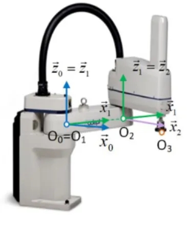
The first step of the DH convention application consists of setting up a coordinate system fixed to each robot rigid part (Figure 4). The position and orientation of the different coordinate systems allow defining the geometrical parameters necessary for the complete definition of the nominal model. These parameters are defined in Table 1 for the first two joints of a SCARA robot when considering 𝑧⃗₀ = 𝑧⃗₁ and 𝑂₀ = 𝑂₁.

Figure 4: Coordinate systems associated with each robot rigid part.

𝑑𝑖 𝜃𝑖 𝑎𝑖 𝛼𝑖

𝑅₀ → 𝑅1 - - 0 0

𝑅1→ 𝑅2 𝑑1 𝑞1 𝑎1 0

𝑅₂→ 𝑅_𝑒 0 𝑞₂ 𝑎₂ 0

Table 1: DH geometric parameters of the studied SCARA robot.

The geometric parameters taken into account by the nominal geometric model of the first two joints of the SCARA robot are the lengths of the arms 1 and 2 (𝑎1 and 𝑎2), the offset

d1 of the end-effector controlled point along the axis 𝑧⃗2 as well as the joint coordinate value applied to the motors (𝑞1, 𝑞2).

2.3 Definition of the SCARA robot nominal model

The definition of the Direct Kinematic Model (DKM) is realized according to transformation matrices such as:

𝐓_𝐍𝟑 𝟎 _{= 𝐓} 𝐍𝟏 𝟎 _𝐓 𝐍𝟐 𝟏 _𝐓 𝐍𝟑 𝟐 ₌ [

cos (𝑞1+ 𝑞2) − sin(𝑞1+ 𝑞2) 0 𝑎2cos(𝑞1+ 𝑞2) + 𝑎1cos (𝑞1) sin(𝑞₁ + 𝑞₂) cos (𝑞₁+ 𝑞₂) 0 𝑎₂sin(𝑞₁+ 𝑞₂) + 𝑎₁sin (𝑞₁)

0 0 1 𝑑₁

0 0 0 1

] (5)

where 𝒋𝐓_𝐍𝒊 is the nominal transformation matrix of coordinate system Ri to coordinate

system R_j.

The last column of this transformation matrix directly provides the coordinates of the nominal position of the point O3 in frame R0:

𝑂₁𝑂_𝑁3 ⃗⃗⃗⃗⃗⃗⃗⃗⃗⃗⃗⃗⃗ = [ 𝐓𝟎 𝐍𝟑(1,4) 𝐓_𝐍𝟑 𝟎 _(2,4) 𝐓_𝐍𝟑 𝟎 (3,4)]_𝑅 0 = [ 𝑎₂cos(𝑞₁+ 𝑞₂) + 𝑎₁cos (𝑞₁) 𝑎₂sin(𝑞₁+ 𝑞₂) + 𝑎₁sin (𝑞₁) 𝑑₁ ] 𝑅0 (6)

This last expression gives the definition of the nominal DKM of the SCARA robot. However, this formalism does not allow integrating orientation defects of the axis 𝑧 ⃗⃗⃗_𝑖 in a plane different from the plane (𝑦⃗_𝑖−1, 𝑧⃗_𝑖−1). The introduction of a complete description of the

orientation of a coordinate system regarding another requires the use of a more complete formalism. The following section introduces such formalism.

3 Geometric defects introduction with a vector method

The geometric behavior of a robot relies on the position and orientation of its joints. For the SCARA robot, introduced defects are linked to the orientation and position of robot rotational joints. The invariant of the rotational joint is a straight-line (rotational joint axis) [18]. Therefore, 4 parameters are introduced for describing this feature, i.e. 2 parameters to define the straight-line orientation and 2 parameters to define a point of this straight-line. In this way, the definition of the direct kinematic model of the SCARA robot requires the identification of 4 parameters, for each rotational joint, which describe the position and orientation of each rotational joint axis in the coordinate system associated with the previous joint axis (Figure 5). Note that, for a prismatic joint just the 2 parameters which define the straight-line orientation are necessary.

The following paragraph introduces the methodology proposed to define these 4 parameters.

(𝑂_𝑖−1, 𝑧⃗_𝑖−1) is the axis of rotational joint i − 1 and (𝑂_𝑖, 𝑧⃗_𝑖) the axis of rotational joint i. 𝑂_𝑖 is the intersection point between plan (𝑂_𝑖−1, 𝑥⃗_𝑖−1, 𝑦⃗_𝑖−1) and the axis of rotational joint i. 𝑥⃗_𝑖−1′ is the direction vector of the straight line (𝑂_𝑖−1𝑂_𝑖), thus 𝑂⃗⃗⃗⃗⃗⃗⃗⃗⃗⃗⃗⃗⃗⃗ = 𝑎_𝑖̇−1𝑂_{𝑖̇ 𝑖−1}𝑥⃗_𝑖−1′. Note the scalar product 𝑥⃗𝑖−1∙ 𝑥⃗𝑖−1′ = cos (𝜃𝑖−1 ). The coordinate system 𝑅𝑖−1 ′ is then defined from the cross product 𝑦⃗𝑖−1′ = 𝑧⃗𝑖−1× 𝑥⃗𝑖−1′. 𝑥⃗𝑖 is along the projection of 𝑥⃗𝑖−1′ in the plan normal to 𝑧⃗𝑖 which contains 𝑂_𝑖. Then the coordinate system 𝑅_𝑖 is defined as 𝑥⃗_𝑖−1′ ∙ 𝑦⃗_𝑖 = 0, 𝑥⃗_𝑖∙ 𝑧⃗_𝑖 = 0 and 𝑦⃗_𝑖 = 𝑧⃗_𝑖 × 𝑥⃗_𝑖

Figure 5: Invariant definition of two rotational joints of a robot arm.

Thus, the rotation matrix allowing defining the orientation of coordinate system 𝑅𝑖−1 ′ in coordinate system 𝑅_𝑖−1 can be written as:

𝐑 𝐢−𝟏 𝐢−𝟏′ = ( cos (𝜃_𝑖−1) − sin(𝜃_𝑖−1) 0 sin (𝜃_𝑖−1) cos (𝜃_𝑖−1) 0 0 0 1 ) (7)

The rotation matrix allowing the expression of coordinate system 𝑅_𝑖 relatively to coordinate system 𝑅_𝑖−1′ is:

𝐑 𝐢−𝟏′ 𝐢 = ( √𝐽_𝑖2+ 𝐾_𝑖2 0 𝐼_𝑖 −𝐼𝑖𝐽𝑖 √𝐽_𝑖2+𝐾_𝑖2 𝐾𝑖 √𝐽_𝑖2+𝐾_𝑖2 𝐽_𝑖 −𝐼𝑖𝐾𝑖 √𝐽_𝑖2+𝐾_𝑖2 −𝐽𝑖 √𝐽_𝑖2+𝐾_𝑖2 𝐾_𝑖 ) (8)

with 𝑧⃗_𝑖 = 𝐼_𝑖𝑥⃗_𝑖−1′ + 𝐽_𝑖𝑦⃗_𝑖−1′ + 𝐾_𝑖𝑧⃗_𝑖−1′, i.e. (𝐼_𝑖, 𝐽_𝑖, 𝐾_𝑖) are the coordinates of 𝑧⃗_𝑖 in frame 𝑅_𝑖−1′, with 𝑥⃗_𝑖−1′ ∙ 𝑦⃗_𝑖 = 0, 𝑥⃗_𝑖∙ 𝑧⃗_𝑖 = 0 and 𝑦⃗_𝑖 = 𝑧⃗_𝑖 × 𝑥⃗_𝑖.

Thus, the identification of the position and the orientation of each rotational joint axis (a straight-line orientation and a point) in the coordinate system associated with the previous axis is performed thanks to 4 independent parameters 𝜃𝑖, 𝑎𝑖, 𝐼𝑖, 𝐽𝑖 and a dependent parameter 𝐾_𝑖 = √1 − (𝐼_𝑖2_{+ 𝐽}

𝑖2). As 𝐾𝑖 is always positive, its imposes the direction of the unit vector of the joint axis. Note that, for a prismatic joint, this formalism is used by canceling 𝜃_𝑖 and 𝑎_𝑖.

The introduced parameters are different from those defined with the DH convention. Indeed, with our methodology, 𝑧⃗_𝑖 axis is not constrained to be in the plane (𝑦⃗𝑖−1, 𝑧⃗𝑖−1). Moreover, 𝑅𝑖 position and orientation are not constrained by the definition of coordinate system 𝑅_𝑖−1.

4 Application to the geometric behavior modeling of the SCARA robot

Applying the strategy previously presented to the first two axes of a SCARA robot, the model presented in Figure 6 is obtained.

First, 𝑧⃗₁ and 𝑧⃗₂ are chosen along the rotation axis of the first two rotational joints of a SCARA robot. Point 𝑂₁ is arbitrary chosen on the first rotational joint axis. For our study, we consider that 𝑅₁ is the robot coordinate system. Coordinate system 𝑅₂(𝑂₂′, 𝑥⃗₂, 𝑦⃗₂, 𝑧⃗₂) is defined according to the methodology presented in section 3. Since the studied system features only 2 degrees of freedom, a coordinate system 𝑅₃ is not introduced, but only a point 𝑂₃ which corresponds to the end-effector control point. The position of this point 𝑂₃ is defined accordingly to the one of point 𝑂_𝑖 in section 3 and the introduction of a new point 𝑂₂. The introduction of this new point 𝑂2 let open the possibility of an offset between chosen point 𝑂1 and end-effector control point 𝑂3. 𝑂1corresponds to a virtual point and, end-effector control point 𝑂₃ can be physically defined and can change accordingly to the used end-effector. Finally, 7 parameters are introduced: 𝜃₁, 𝜃₂, 𝑎₁, 𝑎₂, 𝑑₂, 𝐼₂, 𝐽₂ .

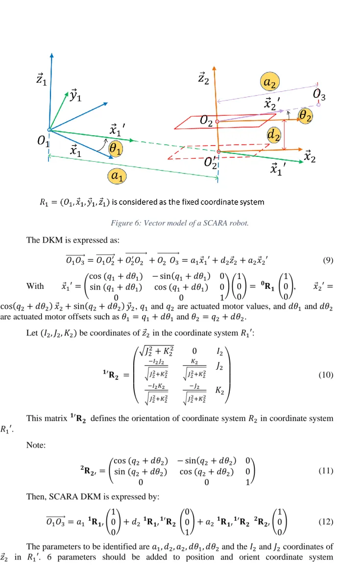
Figure 6: Vector model of a SCARA robot.

The DKM is expressed as: 𝑂1𝑂3 ⃗⃗⃗⃗⃗⃗⃗⃗⃗⃗⃗ = 𝑂⃗⃗⃗⃗⃗⃗⃗⃗⃗⃗ + 𝑂1𝑂2′ ⃗⃗⃗⃗⃗⃗⃗⃗⃗⃗⃗⃗ + 𝑂2′𝑂2 ⃗⃗⃗⃗⃗⃗⃗⃗⃗⃗⃗⃗ = 𝑎2 𝑂3 1𝑥⃗1′ + 𝑑2𝑧⃗2+ 𝑎2𝑥⃗2′ (9) With 𝑥⃗₁′ = ( cos (𝑞₁+ 𝑑𝜃₁) − sin(𝑞₁+ 𝑑𝜃₁) 0 sin (𝑞₁+ 𝑑𝜃₁) cos (𝑞₁+ 𝑑𝜃₁) 0 0 0 1 ) ( 1 0 0 ) = 𝐑𝟎 _𝟏 ( 1 0 0 ), 𝑥⃗₂′ = cos(𝑞2+ 𝑑𝜃2) 𝑥⃗2+ sin(𝑞2+ 𝑑𝜃2) 𝑦⃗2, 𝑞1 and 𝑞2 are actuated motor values, and 𝑑𝜃1 and 𝑑𝜃2 are actuated motor offsets such as 𝜃₁ = 𝑞₁+ 𝑑𝜃₁ and 𝜃₂ = 𝑞₂+ 𝑑𝜃₂.

Let (𝐼₂, 𝐽₂, 𝐾₂) be coordinates of 𝑧⃗₂ in the coordinate system 𝑅₁′:

𝐑 𝟏′ 𝟐 = ( √𝐽₂2+ 𝐾₂2 0 𝐼₂ −𝐼2𝐽2 √𝐽₂2_+𝐾 22 𝐾2 √𝐽₂2_+𝐾 22 𝐽₂ −𝐼2𝐾2 √𝐽22+𝐾22 −𝐽2 √𝐽22+𝐾22 𝐾2 ) (10)

This matrix 𝟏′𝐑_𝟐 defines the orientation of coordinate system 𝑅₂ in coordinate system 𝑅₁′. Note: 𝐑 𝟐 𝟐′= ( cos (𝑞2+ 𝑑𝜃2) − sin(𝑞2+ 𝑑𝜃2) 0 sin (𝑞₂+ 𝑑𝜃₂) cos (𝑞₂+ 𝑑𝜃₂) 0 0 0 1 ) (11)

Then, SCARA DKM is expressed by: 𝑂₁𝑂₃ ⃗⃗⃗⃗⃗⃗⃗⃗⃗⃗⃗ = 𝑎1 𝟏𝐑𝟏′( 1 0 0 ) + 𝑑₂ 𝟏𝐑_𝟏′𝟏′𝐑_𝟐 ( 0 0 1 ) + 𝑎₂ 𝟏𝐑_𝟏′𝟏′𝐑_𝟐 𝟐𝐑_𝟐′( 1 0 0 ) (12) The parameters to be identified are 𝑎₁, 𝑑₂, 𝑎₂, 𝑑𝜃₁, 𝑑𝜃₂ and the 𝐼₂ and 𝐽₂ coordinates of 𝑧⃗₂ in 𝑅₁′. 6 parameters should be added to position and orient coordinate system

𝑅₁(𝑂₁, 𝑥⃗₁, 𝑦⃗₁, 𝑧⃗₁) which is coincident with the robot base coordinate system in the measurement coordinate system.

5 Geometric parameters identification

The identification process is realized with a laser tracker (Leica AT-901) with an uncertainty of 10 μm + 5 μm/m (Figure 7). The target is localized at the extremity of the end-effector. The studied robot joints are moved with harmonic drives. These drives have low backlash [20]. Thus, the influence of backlash in identification process is neglected.

Figure 7: Target measurement with a laser tracker on a SCARA robot.

To directly identify the invariants of robot joints from the laser tracker measurements, the CPA method is used [21][6]. This method ensures to identify each robot rotational joint axis and is described in [21]. This method consists in measuring the tool path followed by the end-effector during a single actuated joint movement (Figure 8). The theoretical tool path is a circle. The normal vector of the plane in which the circle movement lies is the axis vector of the actuated joint, and the circle center is a point of this joint axis. For a robot with N degrees of freedom, N circles should be measured. To minimize the regression errors, the joint positions should be uniformly spaced [21]. The identification accuracy depends on the ability to trace the target on a portion of the total joint travel as large as possible according to the measurement mean visibility [21]. For each value of the joint position, the coordinate of the target is measured in the laser tracker coordinate system. To avoid dynamic phenomena, the robot is stopped during each measurement.

Figure 8: Measured points in the laser tracker coordinate system during a movement of joint 1 and joint 2.

As shown on Figure 8, points 𝐌_𝟏 and 𝐌_𝟐 are the different positions reached by the target during a rotational movement, respectively, of axis 1 or axis 2. The coordinates of the

points measured in laser tracker coordinate system 𝑅_𝐿𝑇(𝑂_𝐿𝑇, 𝑥⃗_𝐿𝑇, 𝑦⃗_𝐿𝑇, 𝑧⃗_𝐿𝑇) are given in appendix A.

In appendix A, we can see that seven positions are measured twice. Between the two measurements, there is a repositioning of the laser tracker target. From these measurements, a maximum target repositioning defect of 0.032 mm is obtained. This error will affecte the identification process.

In this paper, the coordinates of a vector 𝑥⃗ on a given coordinate system 𝑅_𝑖 is noted 𝑥⃗𝑅𝑖_.

The geometric parameters of the SCARA robot are identified from two geometric construction steps:

- From measured points 𝐌_𝟏 obtained during a movement of joint 1, the least-squares plan 𝒫₁ is computed. The normal of this plan ensures to identify the coordinate of 𝑧⃗₁𝑅𝐿𝑇

in the laser tracker coordinate system (Figure 4). The set of points 𝐌_𝟏 are projected in plane 𝒫₁. The least-square circle 𝒞₁ is then computed from these projected points 𝐌_𝟏𝐩. The center of circle 𝒞₁ allows identifying the coordinates of point 𝑂₁𝑅𝐿𝑇

in the laser tracker coordinate system (Figure 4). - From measured points 𝐌_𝟐 obtained during a movement of joint 2, the

least-squares plan 𝒫₂ is computed. The normal of this plan ensure to identify the coordinate of 𝑧⃗₂𝑅𝐿𝑇 _{in laser tracker coordinate system (Figure 4). The set of points}

𝐌_𝟐 are projected in plane 𝒫₂. The least-square circle 𝒞₂ is then computed from these projected points 𝐌_𝟐𝐩. The center of circle 𝒞₂ allows identifying the coordinates of point 𝑂₂𝑅𝐿𝑇

in the laser tracker coordinate system (Figure 4). From these geometric constructions, the geometric parameters introduced in section 4 are identified. In this identification process, we consider that the base coordinate system of the robot is coincident with 𝑅₁, i.e. 𝑅₁ is the fixed coordinate system. The orientation of 𝑥⃗₁ is aligned with 𝑥⃗₁′ when 𝑞₁ = 0, i.e. 𝑑𝜃₁ = 0. The value of 𝑑𝜃₂ is the angle between 𝑥⃗₂ and 𝑥⃗₂′ when 𝑞₂ = 0. 𝑑𝜃₂ is obtained from the angle between 𝑥⃗₂ and 𝑂⃗⃗⃗⃗⃗⃗⃗⃗⃗⃗⃗⃗⃗⃗ when 𝑞₂𝑀_{2𝑝 1} = 0.

𝑎2 is the radius of circle 𝒞2. 𝑂2′ is the intersection point between the straight-line (𝑂2, 𝑧⃗2) and plane 𝒫₁. 𝑑₂ is such that 𝑂₂′_𝑂

2

⃗⃗⃗⃗⃗⃗⃗⃗⃗⃗ = 𝑂⃗⃗⃗⃗⃗⃗⃗⃗⃗⃗⃗ − 𝑂1𝑂2 ⃗⃗⃗⃗⃗⃗⃗⃗⃗⃗ = 𝑑1𝑂2′ 2𝑧⃗2. However, 𝑂⃗⃗⃗⃗⃗⃗⃗⃗⃗⃗ ∙ 𝑧⃗1𝑂2′ 1 = 0. Thus, 𝑑2 is computed from:

𝑑₂ =𝑂⃗⃗⃗⃗⃗⃗⃗⃗⃗⃗⃗⃗∙𝑧⃗1𝑂2 1

𝑧⃗1∙𝑧⃗2 (13)

𝑎1 is the distance between point 𝑂1 and point 𝑂2′ with 𝑎1 = ‖𝑂⃗⃗⃗⃗⃗⃗⃗⃗⃗⃗‖. Moreover, 𝑂1𝑂2′ ⃗⃗⃗⃗⃗⃗⃗⃗⃗⃗ =1𝑂2′ 𝑂₁𝑂₂

⃗⃗⃗⃗⃗⃗⃗⃗⃗⃗⃗ − 𝑑₂𝑧⃗₂. The determination of 𝑥⃗₁′ comes from: 𝑥⃗₁′ =⃗⃗⃗⃗⃗⃗⃗⃗⃗⃗⃗⃗𝑂1𝑂2′

𝑎1 (14)

Thus, 𝑦⃗₁′ = 𝑧⃗₁× 𝑥⃗₁′. We can then deduce 𝐼₂ = 𝑧⃗₂∙ 𝑥⃗₁′, 𝐽₂ = 𝑧⃗₂∙ 𝑦⃗₁′ and 𝐾₂ = 𝑧⃗₂∙ 𝑧⃗₁. Finally, 𝑥⃗₁ = 𝑥⃗₁′ when 𝑞₁= 0 and 𝑦⃗₁ = 𝑧⃗₁× 𝑥⃗₁. Note that coordinate system 𝑅₁ can be identified completely only at the end of the numerical process.

The transformation matrix which expresses coordinate system 𝑅₁ in laser tracker coordinate system is finally defined such as:

𝐓_𝐑𝟏

𝐋𝐓 _{= [𝑥⃗1}𝑅𝐿𝑇 𝑦⃗₁𝑅𝐿𝑇 𝑧⃗₁𝑅𝐿𝑇 𝑂₁𝑅𝐿𝑇

0 0 0 1 ]

The identified values are given in Table 2. Geometric parameters Identified values 𝐓_𝐑𝟏 𝐑𝐋𝐓 [ −0.383553 0.923472 0.009258 −295.393 mm −0.923519 −0.383539 −0.003396 2044.593 mm 0.000415 −0.009853 0.999951 −413.640 mm 0 0 0 1 ] 𝑧⃗₂𝑅1′ _𝐼 2 = 0.000105 𝐽₂ = 0.000114 𝐾₂ = 0.999999 𝑎1 325.034 mm 𝑎2 274.199 mm 𝑑2 0.056 mm 𝑑𝜃₁ 0 rad 𝑑𝜃₂ 0.000279 rad

Table 2: Identified geometric parameters

The residual errors after identification for points 𝐌_𝟏 and 𝐌_𝟐 are given in Figure 9. The maximum residual error value is obtained for a movement of joint 1 and is near 0.069 mm. The mean residual error for a joint 1 movement is 0.030 mm and 0.015 mm for a joint 2 movement. All these values are close to the maximum observed target repositioning defect which is 0.032 mm.

Figure 9: Residual errors on points used for the identification process

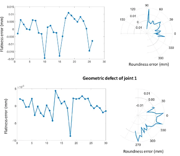
From the identification process, the flatness and roundness of each joint are estimated. These features are technical behavior which characterize the geometric joint behavior (Figure 10). The flatness is estimated by computing the distance between each measured point and the associated least-square plane. The roundness correspond to the distance between each measured point projection and the associated least-square circle. For joint 1, the flatness defect is 0.03 mm and the roundness defect is 0.031 mm. For joint 2, the flatness defect is 0.013 mm and the roundness defect is 0.018 mm.

Figure 10: Geometrical defect of joint 1 and joint 2.

Nine supplementary points 𝐌_𝐯 are measured with the laser tracker for validating realized identification. The coordinates of these points are given in Appendix B. The errors between measured point positions and simulated with identified DKM are less than 0.046 mm (Figure 11). This maximum error is less than the maximum residual error of the identification process which is 0.069 mm in our case study. The inaccuracy of the measurement with the laser tracker, the repeatability of the measurement process, the repeatability of the robot, and the uncompensated defect like joint flatness and roundness explain this error.

Figure 11: Error between the measured position points and the simulated with identified DKM.

To illustrate the benefit of the new vector modeling method introduced in this paper on the final accuracy of geometric model, a comparison between these results and those obtained after an identification of a DH SCARA identified DKM is realized in the following section.

6 Identification of the DH SCARA geometric model

The identification of the DH SCARA geometric model is realized with two viewpoints. The first one brings to realize an identification of just the first order defect (dimensional defect), i.e. 𝑎1, 𝑑2, and 𝑎2. The second one introduces second-order defects which are considered as small displacement. The DH geometric parameters become as in Table 3 if the base coordinate system of the robot is coincident with 𝑅₁, and 𝑅₂′ and 𝑅_𝑒 have the same unit vectors. Thus, two second-order defects are introduced: 𝑑𝛼2 and 𝑑𝜃2.

𝑑𝑖 𝜃𝑖 𝑎𝑖 𝛼𝑖

𝑅₁→𝑅₁′ 0 q₁ 0 0

𝑅₁′→𝑅₂ 0 0 𝑎₁ 𝑑𝛼₂

𝑅2′→𝑅2 𝑑2 𝑞2+ 𝑑𝜃2 𝑎2 0

Table 3: first and second order of DH geometric parameters.

In the following sections, the identification of DH SCARA geometric parameters with only first-order defects is firstly presented. Afterwards, we introduce the identification of DH SCARA geometric parameters with first-order and second-order defects.

6.1 Identification of the DH SCARA geometric parameters reduced to first-order defects

The identification process is realized from points 𝐌_𝟏 and 𝐌_𝟐 measurement. Thus, the position and orientation of coordinate system 𝑅₁ regarding laser tracker coordinate system is the same as in Table 2. All points 𝐌𝟏 are projected in plane 𝒫1. The position of point 𝑂2 is computed from a translation of plane 𝒫₁ with a least square minimization regarding points 𝐌_𝟐.

Geometric parameters Identified values 𝐓_𝐑𝟏 𝐑𝐋𝐓 [ −0.383553 0.923472 0.009258 −295.393 mm −0.923519 −0.383539 −0.003396 2044.593 mm 0.000415 −0.009853 0.999951 −413.640 mm 0 0 0 1 ] 𝑎1 325.034 mm 𝑎₂ 274.199 mm 𝑑₂ 0.022 mm

Table 4: Geometric parameter identified values for DH SCARA first-order geometric model.

The residual errors after identification for points 𝐌_𝟏 and 𝐌_𝟐 are given in Figure 12. The maximum residual error value is obtained for a movement of joint 1 and is near 0.142 mm. The mean residual error for a joint 1 movement is 0.103 mm and 0.070 mm for a joint 2 movement.

Figure 12: Residual errors for DH SCARA first-order geometric model.

The same nine validation points are used to estimate the accuracy benefit brings by the vector geometric model (Figure 13). The errors between measured points position and simulated with identified DKM are less than 0.122 mm. The defect is multiplied by two compared to the proposed vector method.

Figure 13: Error between measured position points and simulated with identified DH first-order DKM.

However, in this DH model only the first-order defects are considered. In the following section, second-order defects are introduced to improve the final accuracy of the robot.

6.2 Identification of the DH SCARA geometric parameters with first and second-order defects

For the case of the DH geometric model with first and second-order defects, the identification process based on CPA cannot be simply implemented. Indeed, with these DH geometric parameters, the only orientation defect between axis 𝑧⃗₁ and 𝑧⃗₂ is a rotation 𝑑𝛼₂ around 𝑥⃗1′. This constraint cannot be easily written in the measurement coordinate system.

In this case, the identification process should be realized by a minimization of a cost function expressed directly from the DKM.

Only matrix 𝟏′𝐑_𝟐 is modified:

𝐑 𝟏′ 𝟐 = ( 1 0 0 0 √1 − 𝑑𝛼₂2 𝑑𝛼₂ 0 −𝑑𝛼₂ √1 − 𝑑𝛼₂2 ) (15)

The SCARA DKM is expressed from equation (12).

The geometric parameters of the SCARA robot are identified in two steps:

- The first step is like the one of section 5. From measured points 𝐌_𝟏 obtained during a movement of joint 1, the least-squares plan 𝒫1 and the least-square circle 𝒞1 are computed. The coordinate of 𝑧⃗1

𝑅𝐿𝑇 _{and of point 𝑂} 1

𝑅𝐿𝑇 _{in the laser}

tracker coordinate system are identified (Figure 4).

- The second step consists of the minimization of a cost function which expresses the difference between the measured coordinate of points 𝐌_𝟐 in the laser coordinate system with the computed vector 𝐎_𝟏𝐎_𝟑𝐑𝐋𝐓 _{= [𝑂}

1𝑂3 ⃗⃗⃗⃗⃗⃗⃗⃗⃗⃗⃗𝑅𝐿𝑇

(𝑞_2𝑖)]:

𝑓_{𝑐𝑜𝑠𝑡} = √∑30 (𝑂⃗⃗⃗⃗⃗⃗⃗⃗⃗⃗⃗⃗⃗ − 𝑂₁𝑀_2𝑖̇ ⃗⃗⃗⃗⃗⃗⃗⃗⃗⃗⃗₁𝑂₃𝑅𝐿𝑇(𝑞_2𝑖))

𝑖=1 (15)

The optimized parameters are the coordinate of 𝑥⃗₁𝑅𝐿𝑇_{, 𝑎}

The optimization numerical process is realized with the function “lsqnonlin” of Matlab®. The optimization stops due to the selected value of the step size tolerance which is 10−10_.

The identified values are given in Table 5.

Geometric parameters Identified values 𝐓_𝐑𝟏 𝐑𝐋𝐓 [ −0.383541 0.923478 0.009258 −295.393 mm −0.923524 −0.383525 −0.003396 2044.593 mm 0.000279 −0.009853 0.999951 −413.640 mm 0 0 0 1 ] 𝑎₁ 325.033 mm 𝑎₂ 274.204 mm 𝑑₂ 0.046 mm 𝑑𝜃₂ 0.000214 rad 𝑑𝛼₂ 0.000231 rad

Table 5: Geometric parameter identified values for DH SCARA first and second-order geometric model.

The residual errors after identification for points 𝐌_𝟏 and 𝐌_𝟐 are given in Figure 14. The maximum residual error value is obtained for a movement of joint 1 and is near 0.087 mm. The mean residual error for a joint 1 movement is 0.041 mm and 0.010 mm for a joint 2 movement.

The same nine validation points are used to estimate the accuracy benefit brings by the vector geometric model (Figure 15). The errors between measured points position and simulated with identified DKM are less than 0.055 mm. The defect is 0.009 mm higher compared to the proposed vector method.

Figure 15: Error between measured position points and simulated with identified DH first and second-order DKM.

Indeed, in this case, a first step, before numerical optimization, should be realized to identify the position and orientation of the coordinate system 𝑅₁ regarding the laser tracker coordinate system. Thus, identification errors should be greater than those obtained with a CPA method due to this first step [22].

To finalize this study, and to illustrate the influence of this DKM parameters, we choose to neglect the term 𝐼₂ in our vector model. Indeed, in the DH first and second-order DKM, this parameter is not introduced. To see the influence of this term, we compare the measured position of the nine validation points with the simulated points with the vector geometric model with 𝐼₂ = 0 (Figure 16).

Figure 16: Error between measured position points and simulated with vector DKM with 𝐼2 =

0.

The errors between the position of the measured points and the studied DKM are less than 0.063 mm. The defect is multiplied by two-thirds compared to the defect obtained with our vector method with 𝐼₂ ≠ 0 and is 0.008 mm higher compared to the DH first and second-order DKM. This last result validates the interest of the proposed vector model and shows the impact of taking into account all the orientation defect of joint axis.

6.3 Summary

To conclude on this section, the proposed vector modeling method improves the accuracy between the real geometric behavior and the simulated geometric behavior even if second-order defects are implemented in the DH geometric model.

Table 6 summarizes the obtained errors between each SCARA robot DKM simulation and the nine measured validation points. Note that the mean error of 0.027 mm obtained with our vector model is close to the measurement process accuracy.

SCARA geometrical model Max error (mm) Mean error (mm)

Vector model 0.046 0.027

DH first-order model 0.122 0.098

DH first and second-order model 0.055 0.033

Table 6: Errors between the position of the measured points and the different test DKM

The other benefit of the proposed vector modeling is the consistency between the vector definition of each joint axis and the CPA identification process. This particularity decreases the influence of the identification numerical process on the inverse kinematic residual error.

7 Conclusion

In this article, a new geometric vector modeling method of a serial kinematic robot consistent with the CPA identification process is presented. This method is based on the definition of position and orientation of the robot joints invariants. The invariant of the rotational joint is a straight-line (rotational joint axis orientation and a point). Thus, four parameters are introduced to position a point and orient a vector which are linked to robot joints. The methodology to define these parameters is introduced. These parameters are identified from a CPA method. This identification ensures to directly identify a vector orientation and a point position with a geometrical point of view.

The application of this method improves the final accuracy of the DKM regarding the DH convention. This method allows controlling the number of introduced geometric parameters even for adjacent parallel joints and also increase the accuracy obtained after the identification process.

These first results are promising regarding the impact of the implementation of this new geometric vector model on the obtained geometric accuracy of serial kinematic robot. Further works should now be conducted to apply this vector geometry modeling method to a closed-loop robot.

References

[1] X. Yang, L. Wu, J. Li, K. Chen, A minimal kinematic model for serial robot calibration using POE formula, Robot. Comput. Integr. Manuf. 30 (2014) 326–334. https://doi.org/10.1016/j.rcim.2013.11.002.

[2] W. Khalil, E. Dombre, Modeling Identification and Control of Robots, Butterworth-Heinemann, 2004. https://doi.org/10.1016/B978-1-903996-66-9.X5000-3.

[3] Y. Wu, A. Klimchik, S. Caro, B. Furet, A. Pashkevich, Geometric calibration of industrial robots using enhanced partial pose measurements and design of experiments, Robot. Comput. Integr. Manuf. 35 (2015) 151–168. https://doi.org/10.1016/j.rcim.2015.03.007.

[4] A. Omodei, G. Legnani, R. Adamini, Three methodologies for the calibration of industrial manipulators: Experimental results on a SCARA robot, J. Robot. Syst. 17 (2000) 291–307. https://doi.org/10.1002/(SICI)1097-4563(200006)17:6<291::AID-ROB1>3.0.CO;2-U.

[5] M. Barati, A.R. Khoogar, M. Nasirian, Estimation and Calibration of Robot Link Parameters with Intelligent Techniques, Iran. J. Electr. Electron. Eng. 7 (2011) 225–234. [6] Y. Cho, H.M. Do, J. Cheong, Screw based kinematic calibration method for robot manipulators with joint compliance using circular point analysis, Robot. Comput. Integr. Manuf. 60 (2019) 63–76. https://doi.org/10.1016/j.rcim.2018.08.001.

[7] J. Denavit, R.S. Hartenberg, A kinematic notation for lower pair mechanism based on matrices, Trans. ASME, J. Appl. Mech. 22 (1955) 215–221.

[8] G. Gogu, P. Coiffet, A. Barraco, Représentation des déplacements des robots, Hermes Science Publications, 1997.

[9] H. Lipkin, A note on Denavit-Hartenberg notation in robotics, in: Proc. ASME Int. Des. Eng. Tech. Conf. Comput. Inf. Eng. Conf. - DETC2005, 2005: pp. 921–926. https://doi.org/10.1115/detc2005-85460.

[10] L.J. Everett, M. Driels, B.W. Mooring, kinematic modelling for robot calibration, in: IEEE Int. Conf. Robot. Autom., 1987: pp. 183–189.

[11] W.K. Veitschegger, C.-H. Wu, Robot Accuracy Analysis Based on Kinematics, IEEE J. Robot. Autom. 3 (1986) 171–179. https://doi.org/10.1109/JRA.1986.1087054.

[12] K. Schröer, S.L. Albright, M. Grethlein, Complete, minimal and model-continuous kinematic models for robot calibration, Robot. Comput. Integr. Manuf. 13 (1997) 73–85. https://doi.org/10.1016/S0736-5845(96)00025-7.

inverse kinematics model with regard to machining behaviour, Mech. Mach. Theory. 44 (2009) 1371–1385. https://doi.org/10.1016/j.mechmachtheory.2008.11.004.

[14] K.C. Gupta, Kinematic Analysis of Manipulators Using the Zero Reference Position Description, Int. J. Rob. Res. 5 (1986) 5–13.

[15] R. He, Y. Zhao, S. Yang, S. Yang, Kinematic-parameter identification for serial-robot calibration based on POE formula, IEEE Trans. Robot. 26 (2010) 411–423. https://doi.org/10.1109/TRO.2010.2047529.

[16] I.M. Chen, G. Yang, C.T. Tan, S.H. Yeo, Local POE model for robot kinematic calibration, Mech. Mach. Theory. 36 (2001) 1215–1239. https://doi.org/10.1016/S0094-114X(01)00048-9.

[17] A. Müller, An overview of formulae for the higher-order kinematics of lower-pair chains with applications in robotics and mechanism theory, Mech. Mach. Theory. 142 (2019). https://doi.org/10.1016/j.mechmachtheory.2019.103594.

[18] A. Clément, C. Valade, A. Rivière, The TTRS: 13 oriented constraints for dimensioning, tolerancing and inspection, Adv. Math. Tools Metrol. III. (1997) 24–42.

[19] W. Khalil, J.-F. Kleinfinger, A new geometric notation for open and close-loop robots, in: Conf. Int. Robot. Autom., USA, 1986: pp. 1174–1179.

[20] B. Siciliano, O. Khatib, Handbook of Robotics, Springer, 2008.

[21] B.W. Mooring, Z.S. Roth, M.R. Driels, Fundamentals of Manipulator Calibration, Wiley-Interscience Publication, 1991.

[22] H. Chanal, F. Paccot, E. Duc, Sensitivity analysis of an overconstrained parallel structure machine tool, the Tripteor X7, Applied Mechanics and Materials, 2012. https://doi.org/10.4028/www.scientific.net/AMM.162.394.

Appendix A: measured points in laser tracker coordinate system for SCARA robot geometric identification 𝑴𝟏𝒊 X Y Z 𝒒𝟏 𝒒𝟐 𝑴𝟐𝒊 X Y Z 𝒒𝟏 𝒒𝟐 1 -746.893 1682.145 -410.693 -15° -30° -407.143 1673.864 -413.804 50° -100° 2 -713.586 1644.155 -411.121 -10° -30° -398.993 1651.404 -413.958 50° -°95 3 -713.584 1644.154 -411.124 -10° -30° -388.905 1629.712 -414.130 50° -9°0 4 -677.066 1609.223 -411.584 -5° -30° -376.952 1608.986 -414.313 50° -85° 5 -637.671 1577.610 -412.056 0° -30° -363.247 1589.378 -414.507 50° -80° 6 -637.667 1577.614 -412.050 0° -30° -347.870 1571.041 -414.720 50° -75° 7 -595.708 1549.577 -412.534 5° -30° -347.872 1571.043 -414.717 50° -75° 8 -551.417 1525.281 -413.035 10° -30° -330.978 1554.116 -414.936 50° -70° 9 -505.156 1504.940 -413.533 15° -30° -312.666 1538.733 -415.162 50° -65° 10 -457.302 1488.706 -414.047 20° -30° -293.079 1524.993 -415.391 50° -60° 11 -457.322 1488.708 -414.027 20° -30° -272.367 1513.017 -415.628 50° -55° 12 -408.285 1476.713 -414.520 25° -30° -250.696 1502.898 -415.870 50° -50° 13 -358.383 1469.036 -415.013 30° -30° -250.709 1502.900 -415.861 50° -50° 14 -307.954 1465.736 -415.491 35° -30° -228.221 1494.696 -416.103 50° -45° 15 -257.432 1466.844 -415.971 40° -30° -205.132 1488.490 -416.343 50° -40° 16 -207.235 1472.356 -416.404 45° -30° -181.579 1484.319 -416.578 50° -35° 17 -157.735 1482.214 -416.817 50° -30° -133.817 1482.200 -417.037 50° -25°

18 -109.238 1496.356 -417.214 55° -30° -109.959 1484.267 -417.263 50° -20° 19 -62.150 1514.673 -417.590 60° -30° -109.989 1484.269 -417.251 50° -20° 20 -16.843 1537.025 -417.93 65° -30° -86.444 1488.406 -417.459 50° -15° 21 -16.850 1537.026 -417.937 65° -30° -63.332 1494.581 -417.655 50° -10° 22 26.304 1563.223 -418.245 70° -30° -40.848 1502.747 -417.838 50° -5° 23 67.023 1593.085 -418.523 75° -30° -19.165 1512.836 -418.008 50° 0° 24 105.006 1626.403 -418.767 80° -30° 1.575 1524.788 -418.162 50° 5° 25 139.966 1662.905 -418.981 85° -30° 1.563 1524.790 -418.164 50° 5° 26 171.539 1702.305 -419.133 90° -30° 21.153 1538.489 -418.302 50° 10° 27 39.488 1553.856 -418.421 50° 15° 28 56.416 1570.765 -418.523 50° 20° 29 71.808 1589.067 -418.606 50° 25° 30 85.547 1608.663 -418.667 50° 30°

Annex B: Measured points for validation of the identification process

𝑴𝒗𝒊 X Y Z 𝒒𝟏 𝒒𝟐 1 _{-465.303 1493.982 -413.932 20° -32°} 2 _{-571.505 1545.766 -412.775 10° -36°} 3 _{-513.505 1496.169 -413.491 10° -20°} 4 _{-567.966 1523.226 -412.897 5° -22°} 5 _{-520.183 1491.571 -413.451 5° -10°} 6 _{-394.761 1453.646 -414.745 13° 0°} 7 _{-12.934 1526.406 -418.046 42° 20°} 8 _{135.229 1638.539 -419.056 61° 18°} 9 _{131.630 1624.232 -419.053 68° 0°}