HAL Id: hal-03093858
https://hal.archives-ouvertes.fr/hal-03093858
Submitted on 4 Jan 2021
HAL is a multi-disciplinary open access
archive for the deposit and dissemination of
sci-entific research documents, whether they are
pub-lished or not. The documents may come from
teaching and research institutions in France or
abroad, or from public or private research centers.
L’archive ouverte pluridisciplinaire HAL, est
destinée au dépôt et à la diffusion de documents
scientifiques de niveau recherche, publiés ou non,
émanant des établissements d’enseignement et de
recherche français ou étrangers, des laboratoires
publics ou privés.
inter-comparison
P. Bakker, E. Stone, S. Charbit, M. Gröger, U. Krebs-Kanzow, S. Ritz, V.
Varma, V. Khon, D. Lunt, U. Mikolajewicz, et al.
To cite this version:
P. Bakker, E. Stone, S. Charbit, M. Gröger, U. Krebs-Kanzow, et al.. Last interglacial temperature
evolution – a model inter-comparison. Climate of the Past, European Geosciences Union (EGU), 2013,
9 (2), pp.605-619. �10.5194/cp-9-605-2013�. �hal-03093858�
Clim. Past, 9, 605–619, 2013 www.clim-past.net/9/605/2013/ doi:10.5194/cp-9-605-2013
© Author(s) 2013. CC Attribution 3.0 License.
EGU Journal Logos (RGB)
Advances in
Geosciences
Open Access
Natural Hazards
and Earth System
Sciences
Open AccessAnnales
Geophysicae
Open AccessNonlinear Processes
in Geophysics
Open AccessAtmospheric
Chemistry
and Physics
Open AccessAtmospheric
Chemistry
and Physics
Open Access DiscussionsAtmospheric
Measurement
Techniques
Open AccessAtmospheric
Measurement
Techniques
Open Access DiscussionsBiogeosciences
Open Access Open Access
Biogeosciences
Discussions
Climate
of the Past
Open Access Open Access
Climate
of the Past
Discussions
Earth System
Dynamics
Open Access Open Access
Earth System
Dynamics
DiscussionsGeoscientific
Instrumentation
Methods and
Data Systems
Open Access
Geoscientific
Instrumentation
Methods and
Data Systems
Open Access DiscussionsGeoscientific
Model Development
Open Access Open Access
Geoscientific
Model Development
DiscussionsHydrology and
Earth System
Sciences
Open AccessHydrology and
Earth System
Sciences
Open Access DiscussionsOcean Science
Open Access Open Access
Ocean Science
DiscussionsSolid Earth
Open Access Open Access
Solid Earth
DiscussionsThe Cryosphere
Open Access Open Access
The Cryosphere
Discussions
Natural Hazards
and Earth System
Sciences
Open Access
Discussions
Last interglacial temperature evolution – a model inter-comparison
P. Bakker1, E. J. Stone2, S. Charbit3, M. Gr¨oger4, U. Krebs-Kanzow5, S. P. Ritz6, V. Varma7, V. Khon5,8, D. J. Lunt2, U. Mikolajewicz4, M. Prange7, H. Renssen1, B. Schneider5, and M. Schulz71Earth & Climate Cluster, Department of Earth Sciences, VU University Amsterdam, 1081HV Amsterdam, the Netherlands 2Bristol Research Initiative for the Dynamic Global Environment (BRIDGE), School of Geographical Sciences,
University of Bristol, Bristol BS8 1SS, UK
3LSCE-CEA-CNRS, Laboratoire des Sciences du climat et de l’environnement (IPSL/LSCE), UMR8212, CEA-CNRS-UVSQ, CE-Saclay, Orme des Merisiers, 91191 Gif-sur-Yvette, France 4Max Planck Institute for Meteorology, Bundesstrasse 53, 20146 Hamburg, Germany
5Institute of Geosciences, Kiel University, Ludewig-Meyn-Str. 10, 24118 Kiel, Germany
6Climate and Environmental Physics, Physics Institute, and Oeschger Centre for Climate Change Research, University of Bern, Bern, Switzerland
7MARUM – Center for Marine Environmental Sciences and Faculty of Geosciences, University of Bremen, Klagenfurter Strasse, 28334 Bremen, Germany
8A.M.Obukhov Institute of Atmospheric Physics RAS, Moscow, Russia
Correspondence to: P. Bakker ([email protected])
Received: 16 July 2012 – Published in Clim. Past Discuss.: 20 September 2012 Revised: 27 February 2013 – Accepted: 1 March 2013 – Published: 11 March 2013
Abstract. There is a growing number of proxy-based recon-structions detailing the climatic changes that occurred during the last interglacial period (LIG). This period is of special interest, because large parts of the globe were characterized by a warmer-than-present-day climate, making this period an interesting test bed for climate models in light of projected global warming. However, mainly because synchronizing the different palaeoclimatic records is difficult, there is no con-sensus on a global picture of LIG temperature changes. Here we present the first model inter-comparison of transient sim-ulations covering the LIG period. By comparing the different simulations, we aim at investigating the common signal in the LIG temperature evolution, investigating the main driv-ing forces behind it and at listdriv-ing the climate feedbacks which cause the most apparent inter-model differences.
The model inter-comparison shows a robust Northern Hemisphere July temperature evolution characterized by a maximum between 130–125 ka BP with temperatures 0.3 to 5.3 K above present day. A Southern Hemisphere July tem-perature maximum, −1.3 to 2.5 K at around 128 ka BP, is only found when changes in the greenhouse gas concen-trations are included. The robustness of simulated January temperatures is large in the Southern Hemisphere and the mid-latitudes of the Northern Hemisphere. For these regions
maximum January temperature anomalies of respectively −1 to 1.2 K and −0.8 to 2.1 K are simulated for the period after 121 ka BP. In both hemispheres these temperature maxima are in line with the maximum in local summer insolation.
In a number of specific regions, a common temperature evolution is not found amongst the models. We show that this is related to feedbacks within the climate system which largely determine the simulated LIG temperature evolution in these regions. Firstly, in the Arctic region, changes in the summer sea-ice cover control the evolution of LIG winter temperatures. Secondly, for the Atlantic region, the Southern Ocean and the North Pacific, possible changes in the charac-teristics of the Atlantic meridional overturning circulation are crucial. Thirdly, the presence of remnant continental ice from the preceding glacial has shown to be important when deter-mining the timing of maximum LIG warmth in the North-ern Hemisphere. Finally, the results reveal that changes in the monsoon regime exert a strong control on the evolution of LIG temperatures over parts of Africa and India. By list-ing these inter-model differences, we provide a startlist-ing point for future proxy-data studies and the sensitivity experiments needed to constrain the climate simulations and to further en-hance our understanding of the temperature evolution of the LIG period.
1 Introduction
To strengthen our confidence in climate models, it is im-portant to assess their ability to realistically simulate a climate different from the present-day climate (Braconnot et al., 2012). The last interglacial period (LIG; ∼ 130 000– 115 000 yr BP) provides an interesting period, because many proxy-based reconstructions show temperatures up to sev-eral degrees higher than present day (CAPE-members, 2006; Turney and Jones, 2010; McKay et al., 2011). However, to date, the evolution of the climate during the LIG is still un-der debate. This is especially true for the establishment of peak interglacial warmth in different regions. For instance, proxy-based reconstructions of surface temperatures from the Norwegian Sea and the North Atlantic are inconclusive on whether peak interglacial warmth occurred in the first or in the second part of the LIG (Bauch and Kandiano, 2007; Nieuwenhove et al., 2011; Govin et al., 2012). The main cause of this uncertainty is the difficulty in establishing a co-herent stratigraphic framework for the LIG period, not only between different regions (e.g. the Norwegian Sea and the North Atlantic) but also between different types of proxy-archives (e.g. speleothems, ice cores, deep-sea cores and lake sediments, e.g. Waelbroeck et al., 2008). Deciphering the evolution of LIG surface temperatures is further complicated by the fact that different types of proxies record different parts of the climatic signal: for instance maximum summer warmth, the number of days above a threshold temperature, the seasonal temperature contrast or average summer tem-peratures (Jones and Mann, 2002; Sirocko et al., 2006). Cli-mate simulations covering the LIG period can be used to fa-cilitate the interpretation of proxy-based temperature recon-structions by providing information on the timing of peak in-terglacial warmth for different months and on possible spatial differences in the evolution of temperatures.
For the LIG period a large number of equilibrium sim-ulations have been analysed (Montoya, 2007; Lunt et al., 2012, and references therein). However, to investigate the evolution of temperatures throughout this period and the tim-ing of maximum warmth (MWT), the transient nature of two of the major forcings, changes in the astronomical con-figuration and changes in the concentrations of the major greenhouse-gases (GHGs), has to be incorporated. A small number of transient climate simulations have previously been performed for the LIG (e.g. Calov et al., 2005; Gr¨oger et al., 2007; Ritz et al., 2011a). Amongst other things they indi-cate the importance of changes in the overturning circulation and the sea-ice cover. These are however known to be highly model-dependent stressing the need for a larger model inter-comparison.
In this study we present the first investigation of the com-mon LIG temperature signal in long, > 10 000 yr, transient simulations performed with seven different climate mod-els. Included are both published LIG transient simulations (Gr¨oger et al., 2007) as well as ones recently performed
within the PMIP3 framework (Paleoclimate Modelling In-tercomparison Project). The climate models used in this inter-comparison study differ in complexity from 2.5-D atmosphere–ocean–vegetation models to general circulation models (GCMs). Some also differ in terms of the climatic forcing and in the components of the climate system which are included (Table 1).
The objectives of this model inter-comparison are the fol-lowing: (1) to determine the transient temperature response to LIG forcings which is common to the different models, (2) to analyse the simulated spatio-temporal response of temper-atures during the LIG and (3) to indicate in which regions climatic feedbacks likely played a crucial role in shaping the LIG temperature evolution. This study provides an important step towards a future comparison of LIG proxy-based recon-structions and transient model simulations.
2 Model simulations
We performed transient LIG climate simulations with a to-tal of seven different climate models of different complexity. In the following model descriptions, we focus only on the relevant differences between the models and the simulation design. For a complete description, see Table 1. In the sec-ond part of this section, an overview of the evolution of the main climate forcings of the LIG period is given in terms of changes in the insolation received by Earth and the changes in the GHG concentrations.
2.1 Description of the climate models 2.1.1 Bern3D
The Bern3D Earth system model of intermediate complex-ity (EMIC) consists of a two-dimensional atmospheric en-ergy and moisture balance model that is coupled to a three-dimensional sea-ice–ocean model. In the atmospheric com-ponent, heat is transported horizontally by diffusion only while moisture is transported by both diffusion and pre-scribed advection (Edwards and Marsh, 2005; M¨uller et al., 2006; Ritz et al., 2011a,b). This means that, compared to other models, the spatial and temporal changes in surface temperatures simulated by the Bern3D model are more di-rectly linked to local changes in the radiative forcing. This simulation includes prescribed changes in the extent of the Northern Hemisphere (NH) continental ice sheets (the Antarctic ice sheet is fixed to present-day configuration be-cause of the coarse resolution of the model at high latitudes). The extent of the NH continental ice sheets is calculated us-ing the benthic δ18O stack (a proxy for global ice volume) of Lisiecki and Raymo (2005) in order to scale the ice sheet between the modern and the Last Glacial Maximum extent (Ritz et al., 2011a). Consequently, until ∼ 125 ka BP rem-nants of the North American and Eurasian ice sheets from the preceding glacial period are prescribed next to the Greenland
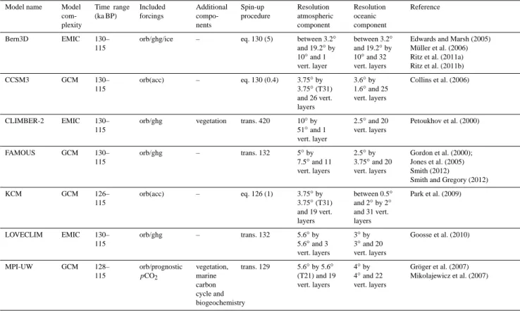
Table 1. List of the main features of the climate models involved in this model inter-comparison. Unless stated otherwise, sea-level, vegetation cover and ice-sheet configuration are fixed to pre-industrial values. The equilibrium GHG values used by CCSM3 and KCM are respectively 272 and 280 ppm for CO2, 622 and 760 ppb for CH4and 259 and 270 ppb for N2O. In column six information about the applied spin-up procedure is given by stating if the spin-up was an equilibrium (eq.) or transient (trans.) simulation, what the corresponding start year (ka BP) of the corresponding forcing scenario is and, in the case of an equilibrium spin-up simulation, what the length (ka) of the spin-up period is (between brackets). The other used acronyms are Earth system model of intermediate complexity (EMIC), general circulation model (GCM), astronomical configuration (orb), astronomical acceleration with a factor of 10 (acc), greenhouse-gas concentrations (ghg), and prescribed changes in ice sheet configuration (ice).
Model name Model com-plexity Time range (ka BP) Included forcings Additional compo-nents Spin-up procedure Resolution atmospheric component Resolution oceanic component Reference Bern3D EMIC 130– 115
orb/ghg/ice – eq. 130 (5) between 3.2◦ and 19.2◦by 10◦and 1 vert. layer between 3.2◦ and 19.2◦by 10◦and 32 vert. layers
Edwards and Marsh (2005) M¨uller et al. (2006) Ritz et al. (2011a) Ritz et al. (2011b) CCSM3 GCM 130– 115 orb(acc) – eq. 130 (0.4) 3.75◦by 3.75◦(T31) and 26 vert. layers 3.6◦by 1.6◦and 25 vert. layers Collins et al. (2006) CLIMBER-2 EMIC 130– 115
orb/ghg vegetation trans. 420 10◦by 51◦and 1 vert. layer 2.5◦and 20 vert. layers Petoukhov et al. (2000) FAMOUS GCM 130– 115 orb/ghg – trans. 132 5◦by 7.5◦and 11 vert. layers 2.5◦by 3.75◦and 20 vert. layers Gordon et al. (2000); Jones et al. (2005) Smith (2012)
Smith and Gregory (2012)
KCM GCM 126– 115 orb(acc) – eq. 126 (1) 3.75◦by 3.75◦(T31) and 19 vert. layers between 0.5◦ and 2◦by 2◦ and 31 vert. layers Park et al. (2009) LOVECLIM EMIC 130– 115 orb/ghg – trans. 132 5.6◦by 5.6◦and 3 vert. layers 3◦by 3◦and 20 vert. layers Goosse et al. (2010) MPI-UW GCM 128– 115 orb/prognostic pCO2 vegetation, marine carbon cycle and biogeochemistry trans. 129 5.6◦by 5.6◦ (T21) and 19 vert. layers 4◦by 4◦and 22 vert. layers Gr¨oger et al. (2007) Mikolajewicz et al. (2007)
ice sheet. Between ∼ 125 ka–121 ka BP, only the Greenland ice sheet remains, and after ∼ 121 ka BP the extent of the North American and Eurasian ice sheets start to increase again. Related to a decrease of the extent of the NH ice sheets, the model includes a meltwater flux from the melting remnant ice sheets into the ocean. During the period when the ice sheets increase, freshwater is removed globally from the ocean surface. Note that the sea level is nonetheless fixed to the present-day situation. The simulation is similar to the one presented by Ritz et al. (2011a) but with the adjusted parameter set of Ritz et al. (2011b).
2.1.2 CCSM3
The CCSM3 (Community Climate System Model, version 3) is a GCM which is composed of four components repre-senting atmosphere (CAM3), ocean (POP), land, and sea ice (Collins et al., 2006). For the simulation in this study, the low-resolution version of CCSM3 is used, which is described in detail by Yeager et al. (2006). The transient simulation has
been carried out with 10 times accelerated astronomical forc-ing (see Sect. 2.3 for details).
2.1.3 CLIMBER-2
The CLIMBER-2 EMIC is a 2.5-D atmosphere–ocean– vegetation model of intermediate complexity (Petoukhov et al., 2000). The atmospheric component is a low-resolution 2.5-D statistical–dynamic model. The oceanic component is a zonally averaged multi-basin (Atlantic, Indian and Pa-cific) model which resolves these basins only in the latitu-dinal direction. CLIMBER-2 includes a thermodynamic sea-ice model that computes the evolution of sea-sea-ice coverage and thickness. Note that, in contrast to most of the simula-tions in this inter-comparison, vegetation is actively simu-lated. This transient simulation is part of a longer simulation covering the last 4 glacial–interglacial cycles (420–0 ka BP) resulting in the initial conditions of this simulation being dif-ferent from the other simulations.
2.1.4 FAMOUS
The FAMOUS GCM (Jones et al., 2005; Smith and Gregory, 2012; Smith, 2012) is a low-resolution version of the HadCM3 GCM (Gordon et al., 2000) with roughly half the horizontal resolution in both the atmosphere and ocean and a longer time step.
2.1.5 Kiel Climate Model
The Kiel Climate Model (KCM) GCM consists of the ECHAM5 atmospheric GCM coupled to the Nucleus for European Modeling of the Ocean (NEMO) ocean–sea-ice GCM (Park et al., 2009). The simulation runs from 126 to 115 ka BP and has been performed with 10 times accelerated astronomical forcing (see Sect. 2.3 for details).
2.1.6 LOVECLIM
The LOVECLIM EMIC includes a simplified atmospheric component and a low-resolution ocean GCM (Goosse et al., 2010).
2.1.7 MPI-UW
The MPI-UW (Max Planck Institute for Meteorology and University of Wisconsin-Madison) Earth system model (Mikolajewicz et al., 2007) is a GCM which consists of the ECHAM3 atmospheric GCM, the Large Scale Geostrophic Ocean (LSG2) GCM including a simple sea-ice model, the Hamburg Ocean Carbon Cycle model (HAMOCC) and the Lund Potsdam Jena dynamical terrestrial vegetation model (LPJ). The latter two components encompass the entire car-bon cycle, which allows for the prognostic calculation of atmospheric pCO2 from the fluxes of HAMOCC and LPJ. In turn, the prognostic pCO2 is then used in the radiative calculations resulting in the GHG forcing in this simula-tion to be different. The atmosphere in this MPI-UW sim-ulation was integrated in periodically synchronous mode. In this method the slow components such as the ocean and veg-etation are integrated for the entire time span, but the fast (and computationally expensive) atmospheric component is integrated only part of the time. In the meantime the ocean model is driven with fluxes from previous synchronous inte-gration periods in combination with an EBM-type damping for small sea surface temperature anomalies. The main un-derlying assumption is that the atmosphere is in statistical equilibrium with the underlying sea-surface temperature and sea ice distribution. The LIG MPI-UW simulation runs from 128 to 115 ka BP (Schurgers et al., 2007; Gr¨oger et al., 2007). Note that in this simulation the vegetation is not fixed at pre-industrial values but actively simulated.
2.2 Evolution of the main climatic forcings of the LIG period
Having an overview of the changes in main climate forcings will allow us to identify if the simulations show a linear re-lation between changes in temperature and the climatic forc-ings or if feedback mechanisms within the climate system are important. The two climate forcings discussed here are the amount of insolation received by Earth and atmospheric GHG concentrations (Figs. 1 and 3; values according to the PMIP3 protocol, http://pmip3.lsce.ipsl.fr/).
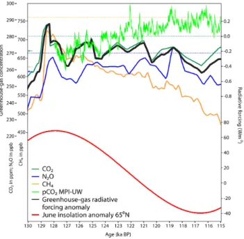
The changes in the amount of insolation received by Earth result from changes in the astronomical configuration. Glob-ally averaged, the anomalies are close to zero for the LIG period. However, changes in the distribution over the dif-ferent latitudes and seasons are not (Berger, 1978). During the first part of the LIG, the NH received more insolation in summer compared to the present-day period. Differences in insolation between both periods exceed 60 W m−2 for June at 65◦N (∼ 130–122 ka BP with a peak around ∼ 127 ka BP; Fig. 1). We do note that maximum insolation anomaly did not occur during the same period for all summer months (Fig. 3; Berger, 2001). For the Southern Hemisphere (SH) summer, the changes in insolation show a strong minimum between 126–123 ka BP while insolation values are just above the present-day ones during the late LIG (< 118 ka BP). The evo-lution of insolation during NH (SH) winter shows a maxi-mum during the late (early) LIG. However, it is important to remember that, at high latitudes (>∼ 67◦), absolute insola-tion and the insolainsola-tion anomalies are close to zero in winter. While all simulations in this model inter-comparison include changes in the astronomical configuration, only some include changes in GHG concentrations (Bern3D, CLIMBER-2, FAMOUS, LOVECLIM and MPI-UW). These are kept constant in the other simulations (CCSM3 and KCM). In accordance with the PMIP3 protocol, the FA-MOUS and LOVECLIM simulations include changes in CO2, CH4 and N2O; the Bern3D simulation only includes changes in CO2 and CH4; and the CLIMBER-2 simula-tion only includes changes in CO2. The GHG concentra-tion values for the LIG period in the PMIP3 protocol are based on ice-core data of Luthi et al. (2008), Loulergue et al. (2008) and Schilt et al. (2010) for respectively CO2, CH4 and N2O. A linear interpolation was applied to these data in order to get a 1 yr time resolution. The GHG concentra-tion changes result in a radiative forcing which increases from low values around 130 ka BP towards maximum val-ues, just above pre-industrial, around 128.5 ka BP. This peak around 128.5 ka BP is sharp and short-lived (i.e. centennial time scale), after which the radiative forcing related to the GHG concentration changes remains approximately constant at values just below pre-industrial (Fig. 1; radiative forcing calculated after Houghton et al., 2001). Note that the radia-tive forcing provided by the changes in the three major GHGs is small, < 0.2 W m−2, compared to the forcing provided by
Fig. 1. In the upper part the changes in the main GHG concentra-tions over the period 130–115 ka BP are depicted. Concentraconcentra-tions are according to the PMIP3 protocol (http://pmip3.lsce.ipsl.fr/), which is based on the ice-core data of Luthi et al. (2008), Louler-gue et al. (2008) and Schilt et al. (2010) for CO2, CH4and N2O respectively. The corresponding pre-industrial values are given by the dotted lines. In constructing the forcing scenarios, a linear in-terpolation was applied to the data to get a 1 yr resolution. The bold black line presents the combined radiative forcing of the three main GHG concentration changes (W m−2; concentrations accord-ing to the PMIP3 protocol; formulation of radiative forcaccord-ing after Houghton et al., 2001). The fixed average LIG GHG concentrations applied in the CCSM3 simulation are depicted by the arrows on the left-hand side of the upper panel. In the MPI-UW simulation, the ra-diative forcing of the GHGs is prognostically calculated from sim-ulated changes in the carbon cycle. The resulting CO2changes are depicted in light green. In the lower part of the figure, the June inso-lation anomaly for 65◦N is given (W m−2relative to pre-industrial values; Berger, 1978).
the insolation changes (Fig. 1). In the simulation performed with the MPI-UW model the pCO2concentration is a prog-nostic variable. Therefore the evolution of the GHG forcing is different from the other simulations (Fig. 1; note that CH4 and N2O are neglected). The simulated GHG evolution in the MPI-UW simulation is characterized by a slow increase between 128–122 ka BP from ∼ 270 ppm towards more sta-ble values of around 285 ppm between 122–115 ka BP. The KCM and CCSM3 simulations have GHG concentrations fixed at pre-industrial and average LIG values respectively (see Table 1 for details).
In all the simulations described in this study, a fixed-day calendar is used. Even though this is common practice in palaeoclimate simulations, it does have a non-negligible ef-fect on the monthly temperature anomalies and has to be
considered when comparing the results with proxy-based re-constructions (Joussaume and Braconnot, 1997; Chen et al., 2011). Another important uncertainty in this study is the age determination of the LIG (Kukla et al., 2002) and the related uncertainty of the applied forcings. However, since all sim-ulations in this inter-comparison applied the same fixed-day calendar method and the same definition of the LIG period, these uncertainties have no impact on the results when we consider the robustness of the simulated temporal evolution of LIG temperatures and the differences between the various simulations (Joussaume and Braconnot, 1997).
2.3 Data processing
All the simulated temperature fields were averaged into 50 yr averages for every month. For the CCSM3 and KCM simu-lations, which are performed with a 10-fold acceleration of the changes in the insolation forcing, averaging over 50 as-tronomical years effectively means an average over only five model years. Therefore, in the CCSM3 and KCM simula-tions only sub-decadal climate variability is filtered out while in the other simulations the variability on multi-decadal time scales is also filtered out. Furthermore, the accelerated orbital forcings might distort the evolution of the deep ocean circu-lation due to its long response time (see also Sect. 3.5). In order to smooth out the artificial noise resulting from the fact that the MPI-UW model was integrated in periodically syn-chronous mode the temperature series have been averaged using a 200 yr window and afterwards linearly interpolated to obtain 50 yr averages. All temperatures of the different sim-ulations were linearly re-gridded onto a common rectangu-lar 1◦×1◦grid. Throughout this manuscript, when dealing with “temperatures” we refer to differences between sim-ulated LIG and pre-industrial near surface air temperature. The pre-industrial temperatures were obtained by averaging over the last 30–100 yr of long (> 500 yr) equilibrium sim-ulations with pre-industrial values for the orbital parameters and GHG concentrations.
3 Results and discussion
In the first part of this section, we focus on the robustness among the models of the simulated LIG temperature evolu-tion and the corresponding LIG temperature maximum. In the second part these results are then related to changes in insolation and GHG concentrations. In part three we dis-cuss the importance of model complexity and resolution and in parts four to seven the impact of climate feedbacks on the simulated LIG temperature evolutions. An assessment of the inter-model differences and spatial patterns in the sim-ulated temperature evolutions can provide valuable infor-mation about the climate system and the important inter-nal feedback mechanisms operating during the LIG period. However, we acknowledge that temperature changes provide
only indirect indications, but a more in-depth investigation of the underlying causes of the inter-model differences is out-side the scope of this manuscript. Nonetheless, we deem that highlighting potentially important climate feedbacks is an es-sential first step towards future sensitivity experiments. 3.1 Simulated robust LIG temperature evolution Because of the seasonal and latitudinal differences in insola-tion, we investigate the robustness of the simulated LIG tem-perature evolution for both January and July in five different latitudinal bands: high and mid-northern latitudes, the trop-ical latitudes and the mid- and high southern latitudes (re-spectively 60◦N–90◦N; 30◦N–60◦N; 30◦S–30◦N; 60◦S– 30◦S and 90◦S–60◦S). These specific latitudinal bands were chosen, because many important feedback processes in the climate system are roughly confined to these regions, e.g. the albedo and sea-ice feedback in the higher latitudes and the monsoon system in the tropical latitudes. With this ap-proach we explicitly assume that longitudinal differences in temperature anomalies are small compared to latitudinal dif-ferences, an assumption of which we will discuss the validity of in the final part of this section. We focus on January and July temperatures to investigate changes in either the cold or warm season. However, we do note that these months do not always represent the warmest or coldest months for a given location.
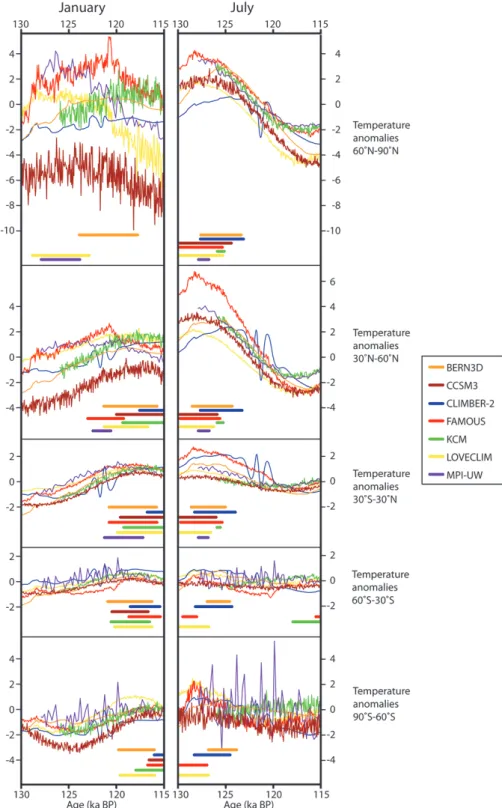
For most latitudinal bands and for both January and July, the different models show LIG temperature evolutions which are comparable in their trend, magnitude of the temperature change and period of maximum warmth (Fig. 2). The robust-ness of the simulated temperatures is depicted by the multi-model mean (MMM) evolution, the corresponding standard deviation (STDEV) and the spread in the MMM period of maximum warmth (Fig. 3). In the high and mid-latitudes of the NH, we find robust peak July MMM temperature anoma-lies of respectively 0.3–3.7 K and 0.7–5.3 K compared to pre-industrial during the time intervals of respectively 128.4– 125.1 ka BP and 129.4–126.3 ka BP (temperature ranges and time intervals are given as the one standard deviation inter-val around the MMM; see caption of Fig. 3 for more details). Simulated January temperature anomalies for the NH mid-latitudes also show a robust trend with a −0.8 to 2.1 K peak between 121.3–117.2 ka BP. Finally, all simulations which include changes in GHG concentrations according to the PMIP3 protocol simulate a period of maximum July warmth for the SH high latitudes of −1.3 to 2.3 K between 129.2– 126 ka BP. The period of maximum January and July LIG warmth and the corresponding temperature anomalies for all latitudinal bands are listed in Table 2.
3.2 Temperature evolution and forcings
The simulated evolution of MMM January and July temper-ature anomalies shows in most cases a clear correspondence
with respectively December and June insolation (Fig. 3). Fur-thermore it is apparent that, when the rate of change of the radiative forcing is large, the model results are robust, but without such a strong trend the resulting temperature evolu-tions tend to differ largely. The latter is especially true for the simulated temperature evolutions in the winter months in high latitude regions which are characterized by a very small insolation forcing. Simulated July temperature anoma-lies for the SH exemplify another finding. We see that the models that include changes in GHG concentrations accord-ing to the PMIP3 protocol (Bern3D, CLIMBER-2, FAMOUS and LOVECLIM) tend to simulate a more distinct temper-ature evolution compared to the simulations that include fixed GHG concentrations (CCSM3 and KCM). The differ-ent GHG forcing evolution applied in the MPI-UW simula-tion mainly impacts the simulated temperatures of the SH high latitudes. These findings highlight the importance of the radiative forcing provided by the changes in GHG concen-trations, though mainly when the magnitude and trend in the insolation forcing is small.
3.3 Model resolution and complexity
The presented model inter-comparison shows that, on long timescales (> 1 ka) and on large spatial scales (latitudinal bands for instance), the differences between EMICs and GCMs in model complexity and model resolution are of minor importance for the simulated temperature evolution. The results do show that the simulated high-frequency cli-mate variability (50–100 yr timescales in this study because of the applied time-averaging) is much larger in the mod-els of higher complexity and resolution. This is not only caused by the higher complexity of the equations of mo-tion in the GCMs but also by the fact that in the simulamo-tions, which include accelerated orbital forcings, the 50 yr averages are actually resulting from only five model years instead of 50. Similarly, because in the MPI-UW simulation the atmo-sphere is integrated in a periodically synchronous way, the 50 yr averages include only a smaller number of years of at-mospheric output, which results in more high-frequency vari-ability. Finally, two of the models (CLIMBER-2 and MPI-UW) include a dynamical terrestrial biosphere component. However, its impact is not easily identified. Schurgers et al. (2007) describe that the vegetation–albedo feedback in MPI-UW causes higher temperatures in the mid- to high latitudes of the NH in the period 128–121 ka BP. Indeed, the MPI-UW temperatures in this latitude band are higher compared to most other models, but in the CLIMBER-2 temperature evolution this is not the case.
3.4 Sea ice and the LIG temperature evolution
While the astronomical and GHG forcings are longitudinally homogeneous, the net effect of changes in the radiative forc-ings and feedback mechanisms within the climate system can
Fig. 2. Simulated 130–115 ka BP January and July surface air temperature anomalies (K) by the seven climate models for five different latitude bands. All temperatures are anomalies relative to pre-industrial values. The temperature series are 50 yr averages. The horizontal bars accompanying the surface temperature anomalies are the periods of maximum warmth for each individual simulation. We define maximum warmth when the temperature is between the upper limit (which is the absolute temperature maximum) and the lower limit (which is the upper limit minus 10 % of the differences between the LIG maximum and minimum values). Note that these calculations are not performed on the 50 yr average-data but on the values from a polynomial which is fitted to the temperature-series in order to get a robust, multi-millennial signal. The individual period of maximum warmth is only shown if the maximum temperature along the polynomial is outside the 1 σ range of the LIG mean. Note that in all simulations shown in this figure a fixed-day calendar was used.
Table 2. List of the MMM timing of the period of maximum LIG warmth (ka BP) and the corresponding temperature anomalies (K) for every latitude band and for both January and July. The time interval of maximum warmth and the corresponding temperature anomalies are calculated as follows: the middle of the period is the time for which the maximum MMM temperature is found, which is in turn the middle temperature given in column seven; the maximum and minimum of the period of maximum warmth are the mid-point ±1 σ , which gives a measure of the spread in the periods of maximum warmth of the individual simulations (for details see captions of Figs. 2 and 3); the temperature range is found by taking the minimum and maximum of the MMM temperatures ±1σ occurring during the period of maximum warmth. In the last column it is given if the mid-point of the MMM period of maximum warmth is outside the 1 σ range of the LIG MMM average temperature. Note that, in all simulations underlying these results, a fixed-day calendar was used.
Maximum Period of maximum warmth (ka BP) Magnitude of maximum warmth (K)
outside
Latitude band Month Maximum Middle Minimum Minimum Middle Maximum 1 σ range
60◦N–90◦N January 123.9 121.0 118.0 −5.8 0.3 1.2 No July 128.4 126.8 125.1 0.3 2.3 3.7 Yes 30◦N–60◦N January 121.3 119.2 117.2 −0.8 0.9 2.1 Yes July 129.4 127.8 126.3 0.7 3.3 5.3 Yes 30◦S–30◦N January 119.2 117.6 116.0 0.6 1.0 1.2 Yes July 129.7 128.3 127.0 0.3 1.5 2.5 Yes 60◦S–30◦S January 121.0 119.8 118.5 −0.3 0.5 1.2 Yes July 130.0 128.4 123.6 −0.7 0.5 1.0 Yes 90◦S–60◦S January 118.4 117.2 115.9 −1.0 0.1 0.7 Yes July 129.2 127.6 126.0 −1.3 1.1 2.3 Yes
result in longitudinal differences in the temperature evolu-tion. To investigate the importance of feedback mechanisms, we focus not only on the temperature evolution of the indi-vidual models and the MMM but also on spatial patterns in the MWT for January and July (Figs. 4 and 5).
For the Arctic Ocean, we find an overall agreement on an early MWT in January (before approximately 123 ka BP) which we relate to a strong feedback involving sea-ice changes. It appears that, in line with findings for the Holocene (Renssen et al., 2005), the early LIG June inso-lation maximum results in a decline in the summer sea-ice cover and thickness and a subsequent decline in the winter sea-ice cover and thickness. This could in turn enhance the heat flux from the ocean to the atmosphere leading to higher atmospheric winter temperatures. Changes in winter insola-tion or in the GHG forcing are not likely the cause since the pattern is clearly confined to the Arctic. Moreover winter in-solation changes in the region are close to zero, and the MPI-UW simulation does show an early January temperature op-timum over the Arctic while it does not include an early LIG GHG forcing maximum. These findings provide strong in-dications that the sea-ice feedback plays an important role in determining the LIG winter temperature evolution in the Arc-tic region. We note, however, that the January MMM STDEV in parts of the Arctic is larger than it is over the surrounding regions, which indicates the model dependency of the sea-ice-temperature feedback (Fig. 5).
Interestingly, the situation in the sea-ice covered regions surrounding Antarctica is rather different. In contrast to the Arctic Ocean, in most of the simulations the MWTs in Jan-uary and July for the sea-ice covered areas of the SH sum-mer do not coincide. Rather, the July MWT in these areas is
∼127 ka BP, while the January MWT is after ∼ 118 ka BP. Also note that no robust January MWT is found over most of the Southern Ocean (Fig. 5) and that the early LIG July MWT over the high latitudes of the SH is only found in 4 of the models (see also Sect. 3.2).
These findings highlight the need for a more thorough investigation to establish the importance of sea-ice cover changes for the evolution of LIG temperatures and the possi-ble differences between the Arctic and Antarctic.
3.5 The AMOC and the LIG temperature evolution Several of the simulations in this inter-comparison study show large, abrupt changes in surface temperature anoma-lies that cannot easily be related to changes in the forcings. However, we are able to relate some of them to changes in the strength of Atlantic meridional overturning circula-tion (AMOC) by comparing the timing of these temperature changes with the simulated AMOC evolution (Fig. 6). The strength of the AMOC has a large impact on the exchange of heat between the SH and NH and on the exchange of heat between the atmosphere and the ocean. However, the strength of the AMOC can change rapidly because of its po-tentially bi-stable behaviour (Stommel, 1961). Moreover, its strength, stability and locations of the main convective re-gions are highly model-dependent. As a result, the simulated LIG evolution of characteristics of the AMOC differs largely between the models. In the following we will discuss the ap-parent relation between the simulated LIG temperatures and the strength of the AMOC. Note, however, that these are in-direct indications only and additional sensitivity experiments would be necessary to confirm the connection and understand the underlying mechanisms.
Fig. 3.Simulated 130–115 ka BP January and July MMM surface air temperature anomalies (K; black) and STDEV (1 σ ; grey) for five different latitude bands. The MMMs and STDEVs are calculated using the temperature time series shown in Fig. 2. Note that the number of models used in calculating the MMM and STDEV differs per latitude band and per time interval, because Bern3D has latitudinal grid limits at 76◦N and 76◦S and the MPI-UW and KCM simulations run only from respectively 128–115 ka BP and 126–115 ka BP. Furthermore, the applied orbital acceleration in the CCSM3 and KCM and the applied periodically synchronous integration in MPI-UW impact the size of the STDEV (see also Sect. 2.3). The vertical grey lines give the MMM mid-points of the period of maximum warmth. The width of the corresponding grey box gives the spread in the periods of maximum warmth of the individual simula-tions (1 σ ) while its height gives an indication of the number of simulasimula-tions used in the calculation (see Fig. 2). This model spread is further illustrated by the depicted mid-points of the individual periods of maximum warmth (see Fig. 2 for the corresponding colour coding). The period of maximum warmth is only shown if for at least four in-dividual simulations we find a maximum temperature along the polynomial which is outside the 1 σ range of the model individual LIG mean. Also shown in this figure are the corresponding 130–115 ka BP insolation anomalies for the mid-latitude of the chosen latitude bands (W m−2). The left-hand column gives the December (yellow), January (orange) and February (red) insolation anomalies, while in the right-hand col-umn insolation anomalies for June (yellow), July (orange) and August (red) are given. All values are anomalies relative to pre-industrial values.
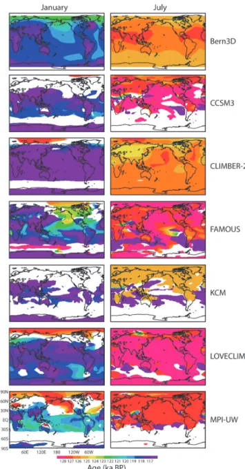
Fig. 4. Timing of the simulated January and July LIG temper-ature maximum (MWT) in the different simulations. The timing (ka BP) is the period for which the highest 50 yr average temper-ature anomalies are found along a polynomial fitted to the indi-vidual temperature time series for every grid cell. Values are only shown if the highest temperatures are outside the 2 σ range of the mean LIG temperature anomaly for the specific grid cell. Note that Bern3D has latitudinal grid limits at 76◦N and 76◦S. Furthermore, the MPI-UW and KCM simulations run from 128–115 ka BP and 126–115 ka BP respectively. Therefore, the colour corresponding to a timing of respectively 128–127 ka BP and 126–125 ka BP should be interpreted as being > 127 ka BP or > 125 ka BP in the case of the MPI-UW and KCM simulations. In all simulations shown in this figure, a fixed-day calendar was used.
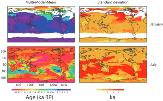
Fig. 5. MMM (left) and STDEV (right) of the timing of maximum warmth (MWT) for January and July based on the individual simulations as shown in Fig. 4. The standard deviation gives a measure of the spread in the simulated timing of maximum warmth between the different models (ka; 2 σ ). The MMM and STDEV are only shown if in at least four individual simulations we find a maximum temperature along a fitted polynomial which is outside the 1 σ range of the model individual LIG mean (see Fig. 4). Note that the calculations do not include the Bern3D model north of 76◦N and south of 76◦S in accordance with its latitudinal grid limits. The calculations do include the KCM and MPI-UW simulations. However, since they only run from 126–115 ka BP and 128–115 ka BP respectively, this might slightly offset the results shown in this figure.
The FAMOUS model simulates an abrupt decline in Jan-uary NH temperatures around 121 ka BP (Fig. 2), a signal which originates largely from the northern Pacific (not shown here). This abrupt decline is followed within centuries by an abrupt increase of both January and July temperatures at mid-southern latitudes. Furthermore, the FAMOUS sim-ulation shows an anomalous January MWT pattern over the Southern Ocean and over the northern and north-eastern Pa-cific (Fig. 4). The LIG simulation performed with the FA-MOUS model is characterized by two different modes of the AMOC. Between 130–121 ka BP a weak AMOC is simu-lated (∼ 70 % weaker compared to the strong mode of the AMOC; Fig. 6) and the main site of deep convection is lo-cated in the North Pacific (not shown). Around 121 ka BP the AMOC switches to a strong mode which is character-ized by deep convection mainly taking place in the North Atlantic. The changes in the global overturning circulation around 121 ka BP are likely related to the concurrent temper-ature changes and the anomalous MWT in parts of the North Pacific and Southern Ocean, and the mechanisms behind it should be investigated more thoroughly in a future study.
The second simulation showing abrupt temperature changes which can be related to changes in the AMOC strength is LOVECLIM. The simulation performed with LOVECLIM shows an abrupt January cooling at around 120 ka BP at high northern latitudes (Fig. 2). Accompany-ing this temperature shift is a region of anomalous timAccompany-ing of winter warmth in the Labrador Sea (Fig. 4). The evolu-tion of the AMOC strength in the LOVECLIM simulaevolu-tion is characterized by an abrupt weakening by about 15 % around 120 ka BP (compared to the period before), after which the AMOC remains unstable (Fig. 6). The simulated changes in AMOC strength in the LOVECLIM model are related to pe-riods of weakened convection in the Irminger Sea (not shown here). Two quasi-stable AMOC modes have already been de-scribed for the LOVECLIM model by Schulz et al. (2007). An interesting question is whether the mode transitions in the FAMOUS and LOVECLIM simulations are determined by an external forcing or do they occur by chance (stochasti-cally) both at around 120 ka BP. Running the ensemble simu-lations necessary to answer this question is however outside the scope of the manuscript.
The Bern3D model shows a anomalous spatial pattern over the Labrador Sea with a timing of maximum win-ter warmth clearly offset from the surrounding areas. As mentioned before, the Bern3D model incorporates both
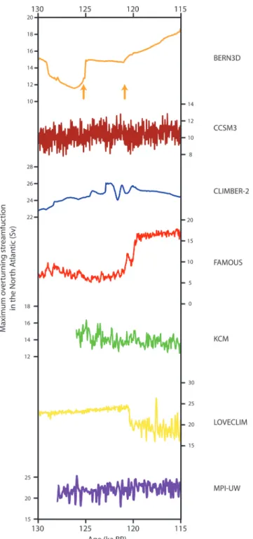
Fig. 6. Simulated LIG evolution of the strength of the AMOC in the seven different simulations. The maximum overturning stream function in the North Atlantic (Sv) is used to indicate the strength of the AMOC. All values are averages over 50 astronomical years. The arrows in the top panel indicate the moment when the meltwa-ter flux from the remnant ice sheets into the oceans in the Bern3D simulation ceases (∼ 125 ka BP) and when continental ice sheets on the NH start to expand again (∼ 121 ka BP).
prescribed remnant ice sheets and a related meltwater flux entering into the ocean between roughly 130–125 ka BP (see Sect. 2.1.1). Concurrent with this melt flux, a some-what weakened AMOC is simulated for the period 129– 125 ka BP (20–30 % compared to the period 125–121 ka BP during which no freshwater flux is applied; Fig. 6). After 121 ka BP, growth of the NH continental ice sheets is pre-scribed in the Bern3D simulation. To compensate for this, a volume of freshwater is removed globally from the ocean sur-face. Therefore the surface ocean becomes more dense (not shown), and as a result an increase of the AMOC strength is simulated. The timing of maximum winter warmth over the Labrador region, after 117 ka BP, corresponds to the period of maximum AMOC strength. Note however that, compared to the simulations performed with FAMOUS and LOVECLIM, the simulated changes in the AMOC strength in Bern3D do not seem to have such a clear impact on the simulated LIG temperature evolution (Fig. 2).
The last simulation showing abrupt changes in the LIG temperature evolution which can be related to changes in the AMOC strength is CLIMBER-2. In the period between 123–120 ka BP, we see large temperature fluctuations with a duration of about 1 ka (Fig. 2). Similar shifts are apparent in the simulated strength of the AMOC in the CLIMBER-2 simulation (Fig. 6). Interestingly and in contrast to the three simulations described above, while the changes in AMOC strength are relatively small, they cause major, ∼ 4 K shifts in the NH mid-latitude temperatures.
Of the remaining three models, the KCM and CCSM3 simulations show a more stable AMOC throughout the LIG. But note that the KCM and CCSM3 simulations have been performed with an acceleration technique, and therefore this analysis does not allow us to determine if the apparent sta-bility of the AMOC strength is an actual model character-istic or an artefact of the applied acceleration technique. Finally, the MPI-UW simulation shows fluctuations in the AMOC strength (Fig. 6) and corresponding high-frequency temperature variability in the SH (Fig. 2) which are related to multi-centennial variability in Southern Ocean deep con-vection (not shown).
Regardless of the exact mechanisms causing the changes in the AMOC in the different simulations, these results show the importance of the evolution of the configuration and strength of the AMOC for the simulated evolution of LIG temperature anomalies. This appears to be especially true for regions like the North Atlantic, the Labrador Sea, the Norwegian and the Barents seas, the north-eastern Pacific and possibly the Southern Ocean. In order to simulate a more robust LIG temperature evolution for these regions, stronger constraints are needed on how the configuration of the AMOC evolved and if mode-switches occurred during the LIG, which is, to date, still inconclusive (Nieuwenhove et al., 2011).
3.6 Ice sheets and the LIG temperature evolution In the transient LIG simulation performed with the Bern3D model, changes in the size of the continental NH ice sheets were prescribed. According to the method applied by Ritz et al. (2011a) to reconstruct remnant ice sheets, parts of the NH continents remained glaciated until ∼ 125 ka BP (see Sect. 2.1.1). Therefore, this simulation provides the possibil-ity to investigate the impact of remnant ice sheets on the LIG temperature evolution. The impact of remnant ice is most clearly visible in the simulated July temperature evolution in high northern latitudes. The peak warmth simulated by the Bern3D model occurs several thousands of years later than in most of the other simulations (Fig. 2). Note, however, that it is not easy to distinguish between the impact of remnant ice and the weakening of the AMOC. It is to be expected that remnant ice has a larger impact on July temperatures, while the changes in the strength of the AMOC more likely result in changes in January temperatures. However, this is not clear from our results.
Renssen et al. (2009) have shown for the present inter-glacial period that remnant ice sheets had a profound influ-ence on the surrounding regions, delaying the thermal max-imum to several thousands of years after the insolation op-timum. The simulation performed with the Bern3D model, even though of lower resolution than the model used by Renssen et al. (2009), indicates a similar delay of maximum warmth. However, a thorough comparison of several sim-ulations including remnant ice sheets is needed to retrieve a more robust signal of the impact of remnant ice on the LIG temperature evolution. Such a model inter-comparison is however further complicated by the fact that different re-constructions of the changes in altitude and extent of the ice sheets during the LIG are still inconclusive. According to Kopp et al. (2009), maximum LIG global sea level was at least 6 m above present day. A small part of this can be ac-counted for through thermal expansion of the ocean waters (McKay et al., 2011) and a loss of mountain glaciers. But the relative contributions of the Greenland and Antarctic ice sheets are still heavily debated (Dutton and Lambeck, 2012, and references therein).
3.7 The monsoon and the simulated LIG temperature evolution
Finally we examine the anomalous pattern in simulated LIG temperatures in the regions centered on the Sahel and on India. The simulated July MMM MWT over these regions is clearly later than the surrounding regions (Fig. 5). How-ever, the large STDEV value indicates that this anomalous pattern is only simulated by some of the models. Maxi-mum July temperatures over the regions centered on the Sa-hel and India are reached before 126 ka BP in Bern3D and LOVECLIM, around 124 ka BP in CLIMBER-2 and after 120 ka BP in CCSM3, KCM and MPI-UW. Again another
pattern is simulated by the FAMOUS model, showing an early (> 127 ka BP) MWT over the Sahel but a late (< 118 ka BP) MWT over parts of India (Fig. 4). Solely based on the geographical distribution of these anomalous MWT patterns, we relate them to changes in the monsoon sys-tem. There are several important differences between the different models which can at least partly explain the large STDEV in these areas. Most of the GCMs in this model inter-comparison (CCSM3, KCM and MPI-UW) simulate a MWT in the Indian and African monsoon regions which is delayed with respect to the insolation forcing. This can be explained by strong feedbacks between the insolation, land evapotranspiration and cloudiness as described by Mulitza et al. (2008). In the MPI-UW simulation this negative feed-back related to clouds and precipitation is partly compen-sated by the positive vegetation–albedo feedback in these regions as savanna is partly replaced by tropical and tem-perate forests (not shown). The EMICs in this model inter-comparison have difficulty to realistically simulate changes in the monsoon system because of their low resolution and simplified atmospheric physics and dynamics. For instance in the Bern3D model, the moisture transport is driven by fixed, zonally averaged winds which inhibit any changes in the monsoon system to be simulated. In LOVECLIM, the simulated changes in the tropical regions should also be treated with care since the results are strongly affected by the quasi-geostrophic nature of its atmosphere and the fixed cloud cover. This model inter-comparison shows the impor-tance of changes in monsoon systems for the evolution of LIG temperatures in regions centered on the Sahel and India even though the exact climate change mechanisms at work for these specific regions are likely different in the different simulations. Furthermore, the model inter-comparison has shown that the LIG temperature evolution in monsoon re-gions tends to be very different between EMICs and GCMs.
4 Summary
In this manuscript we have presented the first model inter-comparison study of long, > 10 ka transient simulations cov-ering the LIG period with a total of seven different climate models. The aim has been to determine the common tran-sient temperature response to the LIG forcings and to indi-cate which feedbacks appear to play a crucial role. Despite large differences between the incorporated climate models and the forcings of the different simulations, the results show for large parts of the globe a robust evolution of LIG Jan-uary and July surface air temperature anomalies compared to pre-industrial values. The main findings are outlined below.
– Simulated July temperature anomalies for the NH show a robust temperature maximum between 130–125 ka BP with a magnitude ranging from 0.3–5.3 K.
– Peak January warmth is found for the NH mid-latitudes (30◦N–60◦N) between 121–117 ka BP with anomalies of −0.8 to 2.1 K, but for the NH high latitudes (60◦N– 90◦N) the results of the simulations are inconclusive. – Over the Arctic Ocean a robust 128–126 ka BP timing
of peak January warmth is found.
– The simulated January temperature evolution for the SH shows a robust temperature maximum after 121 ka BP with corresponding temperature anomalies of −1 to 1.2 K.
– The July temperature maximum for the SH is found be-tween 130–124 ka BP but only in the four simulations which include prescribed changes in GHG concentra-tions.
– The simulations show a close relation between changes in insolation and temperature in both summer and win-ter for almost all latitudes. There are two main excep-tions: NH high-latitude winter temperature changes re-sult largely from sea-ice related feedbacks and are there-fore highly model-dependent; and SH mid- to high-latitude winter temperature changes appear strongly af-fected by changes in GHG concentrations.
– The impact of model complexity and or resolution is of minor importance for the simulated temperature evo-lution over longer (> 1 ka) timescales and large spatial scales.
Based on the differences between the simulations and the investigation of regional patterns in the timing of maximum warmth, we found that several climate feedbacks are likely to be of major importance when simulating the evolution of LIG temperatures: the sea-ice feedback, changes in the strength and configuration of the AMOC, remnants of NH continental ice sheets and changes in the monsoon system.
Our results yield important information for future model– data comparison studies by detailing the following: (1) in which regions the model results are robust and can thus potentially help interpret temperature reconstructions; (2) for which regions more constraints on the LIG climate are needed before a successful model–data comparison can be achieved, because the simulated temperature changes are closely linked to model-dependent climate feedbacks. More-over, our findings will serve as the starting point for a number of sensitivity studies that will be performed to determine ex-actly how important these feedbacks are and to investigate the mechanisms behind them.
Acknowledgements. We thank the anonymous reviewers and the editor Masa Kageyama. This is Past4Future contribution no. 32. The research leading to these results has received funding from the European Union’s Seventh Framework programme
(FP7/2007–2013) under grant agreement no. 243908, “Past4Future. Climate change – Learning from the past climate”. CCSM3 simulations were performed on the SGI Altix supercomputer of the Norddeutscher Verbund fuer Hoch- und Hoechstleistungsrechnen (HLRN). Furthermore, we would like to thank Bette Otto-Bliesner from the National Center for Atmospheric Research (Boulder, USA) for her helpful suggestions.
Edited by: M. Kageyama
References
Bauch, H. A. and Kandiano, E. S.: Evidence for early warm-ing and coolwarm-ing in North Atlantic surface waters dur-ing the last interglacial, Paleoceanography, 22, PA1201, doi:10.1029/2005PA001252, 2007.
Berger, A.: Long-term variations of caloric insolation resulting from the earth’s orbital elements, Quaternary Res., 9, 139–167, 1978. Berger, A.: The role of CO2, sea-level and vegetation during the Milankovitch-forced glacial-interglacial cycles, in: Geosphere-Biosphere Interactions and Climate, edited by: Bengtsson, L. O. and Hammer, C. U., 119–146, Cambridge University Press, New York, 2001.
Braconnot, P., Harrison, S. P., Kageyama, M., Bartlein, P. J., Masson-Delmotte, V., Abe-Ouchi, A., Otto-Bliesner, B., and Zhao, Y.: Evaluation of climate models using palaeoclimatic data, Nature Clim. Change, 2, 417–424, doi:10.1038/nclimate1456, 2012.
Calov, R., Ganopolski, A., Claussen, M., Petoukhov, V., and Greve, R.: Transient simulation of the last glacial inception. Part I: glacial inception as a bifurcation in the climate system, Clim. Dynam., 24, 545–561, 2005.
CAPE-members – Anderson, P., Bennike, O., Bigelow, N., Brigham-Grette, J., Duvall, M., Edwards, M., Fr´echette, B., Funder, S., Johnsen, S., Knies, J., Koerner, R., Lozhkin, A., MacDonald, G., Marshall, S., Matthiessen, J., Miller, G., Montoya, M., Muhs, D., Otto-Bliesner, B., Overpeck, J., Reeh, N., Sejrup, H. P., Turner, C., and Velichko, A.: Last Interglacial Arctic warmth confirms polar amplification of climate change, Quaternary Sci. Rev., 25, 1383–1400, doi:10.1016/j.quascirev.2006.01.033, 2006.
Chen, G., Kutzbach, J. E., Gallimore, R., and Liu, Z.: Cal-endar effect on phase study in paleoclimate transient sim-ulation with orbital forcing, Clim. Dynam., 37, 1949–1960, doi:10.1007/s00382-010-0944-6, 2011.
Collins, W. D., Bitz, C. M., Blackmon, M. L., Bonan, G. B., Bretherton, C. S., Carton, J. A., Chang, P., Doney, S. C., Hack, J. J., Henderson, T. B., Kiehl, J. T., Large, W. G., McKenna, D. S., Santer, B. D., and Smith, R. D.: The Community Climate System Model Version 3 (CCSM3), J. Climate, 19, 2122–2143, doi:10.1175/JCLI3761.1, 2006.
Dutton, A. and Lambeck, K.: Ice Volume and Sea Level During the Last Interglacial, Science, 337, 216–219, doi:10.1126/science.1205749, 2012.
Edwards, N. R. and Marsh, R.: Uncertainties due to transport-parameter sensitivity in an efficient 3-D ocean-climate model, Clim. Dynam., 24, 415–433, doi:10.1007/s00382-004-0508-8, 2005.
Goosse, H., Brovkin, V., Fichefet, T., Haarsma, R., Huybrechts, P., Jongma, J., Mouchet, A., Selten, F., Barriat, P.-Y., Campin, J.-M., Deleersnijder, E., Driesschaert, E., Goelzer, H., Janssens, I., Loutre, M.-F., Morales Maqueda, M. A., Opsteegh, T., Mathieu, P.-P., Munhoven, G., Pettersson, E. J., Renssen, H., Roche, D. M., Schaeffer, M., Tartinville, B., Timmermann, A., and Weber, S. L.: Description of the Earth system model of intermediate complex-ity LOVECLIM version 1.2, Geosci. Model Dev., 3, 603–633, doi:10.5194/gmd-3-603-2010, 2010.
Gordon, C., Cooper, C., Senior, C. A., Banks, H., Gregory, J. M., Johns, T. C., Mitchell, J. F. B., and Wood, R. A.: The simulation of SST, sea ice extents and ocean heat transports in a version of the Hadley Centre coupled model without flux adjustments, Clim. Dynam., 16, 147–168, doi:10.1007/s003820050010, 2000. Govin, A., Braconnot, P., Capron, E., Cortijo, E., Duplessy, J.-C., Jansen, E., Labeyrie, L., Landais, A., Marti, O., Michel, E., Mos-quet, E., Risebrobakken, B., Swingedouw, D., and Waelbroeck, C.: Persistent influence of ice sheet melting on high northern lat-itude climate during the early Last Interglacial, Clim. Past, 8, 483–507, doi:10.5194/cp-8-483-2012, 2012.
Gr¨oger, M., Maier-Reimer, E., Mikolajewicz, U., Schurgers, G., Vizca´eno, M., and Winguth, A.: Changes in the hydrological cycle, ocean circulation, and carbon/nutrient cycling during the last interglacial and glacial transition, Paleoceanography, 22, PA4205, doi:10.1029/2006PA001375, 2007.
Houghton, J., Ding, Y., Griggs, D., Noguer, M., van der Linden, P., Dai, X., Maskell, K., and Johnson, C.: Climate Change 2001: The Scientific Basis, Contribution of Working Group I to the Third Assessment Report of the Intergovernmental Panel on Climate Change, Cambridge University Press, 2001.
Jones, P. D. and Mann, M. E.: Climate over past millennia, Rev. Geophys., 42, RG2002, doi:10.1029/2003RG000143, 2002. Jones, P. D., Gregory, J., Thorpe, R., Cox, P., Murphy, J., Sexton, D.,
and Valdes, P.: Systematic Optimisation and climate simulations of FAMOUS, a fast version of HadCM3, Clim. Dynam., 25, 189– 204, doi:10.1007/s00382-005-0027-2, 2005.
Joussaume, S. and Braconnot, P.: Sensitivity of paleoclimate simu-lation results to season definitions, J. Geophys. Res., 102, 1943– 1956, doi:10.1029/96JD01989, 1997.
Kopp, R. E., Simons, F. J., Mitrovica, J. X., Maloof, A. C., and Oppenheimer, M.: Probabilistic assessment of sea level during the last interglacial stage, Nature, 462, 863–867, doi:10.1038/nature08686, 2009.
Kukla, G. J., Bender, M. L., de Beaulieu, J.-L., Bond, G., Broecker, W. S., Cleveringa, P., Gavin, J. E., Herbert, T. D., Imbrie, J., Jouzel, J., Keigwin, L. D., Knudsen, K.-L., McManus, J. F., Merkt, J., Muhs, D. R., M¨uller, H., Poore, R. Z., Porter, S. C., Seret, G., Shackleton, N. J., Turner, C., Tzedakis, P. C., and Winograd, I. J.: Last Interglacial Climates, Quaternary Res., 58, 2–13, doi:10.1006/qres.2001.2316, 2002.
Lisiecki, L. E. and Raymo, M. E.: A Pliocene-Pleistocene stack of 57 globally distributed benthic δ18O records, Paleoceanography, 20, PA1003, doi:10.1029/2004PA001071, 2005.
Loulergue, L., Schilt, A., Spahni, R., Masson-Delmotte, V., Blu-nier, T., Lemieux, B., Barnola, J.-M., Raynaud, D., Stocker, T. F., and Chappellaz, J.: Orbital and millennial-scale features of at-mospheric CH4over the past 800,000[thinsp]years, Nature, 453, 383–386, doi:10.1038/nature06950, 2008.
Lunt, D. J., Abe-Ouchi, A., Bakker, P., Berger, A., Braconnot, P., Charbit, S., Fischer, N., Herold, N., Jungclaus, J. H., Khon, V. C., Krebs-Kanzow, U., Lohmann, G., Otto-Bliesner, B., Park, W., Pfeiffer, M., Prange, M., Rachmayani, R., Renssen, H., Rosen-bloom, N., Schneider, B., Stone, E. J., Takahashi, K., Wei, W., and Yin, Q.: A multi-model assessment of last interglacial tem-peratures, Clim. Past Discuss., 8, 3657–3691, doi:10.5194/cpd-8-3657-2012, 2012.
Luthi, D., Le Floch, M., Bereiter, B., Blunier, T., Barnola, J.-M., Siegenthaler, U., Raynaud, D., Jouzel, J., Fischer, H., Kawamura, K., and Stocker, T. F.: High-resolution carbon dioxide concen-tration record 650,000–800,000[thinsp]years before present, Na-ture, 453, 379–382, doi:10.1038/nature06949, 2008.
McKay, N. P., Overpeck, J. T., and Otto-Bliesner, B. L.: The role of ocean thermal expansion in Last Interglacial sea level rise, Geophys. Res. Lett., 38, L14605, doi:10.1029/2011GL048280, 2011.
Mikolajewicz, U., Gr¨oger, M., Maier-Reimer, E., Schurgers, G., Vizca´ıno, M., and Winguth, A.: Long-term effects of anthro-pogenic CO2emissions simulated with a complex earth system model, Clim. Dynam., 28, 599–633, doi:10.1007/s00382-006-0204-y, 2007.
Montoya, M.: Paleoclimate modeling, The Last Interglacial, Else-vier, 1916–1927, doi:10.1016/B0-44-452747-8/00033-8, 2007. Mulitza, S., Prange, M., Stuut, J., Zabel, M., von Dobeneck,
T., Itambi, A. C., Nizou, J., Schulz, M., and Wefer, G.: Sahel megadroughts triggered by glacial slowdowns of At-lantic meridional overturning, Paleoceanography, 23, PA4206, doi:10.1029/2008PA001637, 2008.
M¨uller, S. A., Joos, F., Edwards, N. R., and Stocker, T. F.: Wa-ter Mass Distribution and Ventilation Time Scales in a Cost-Efficient, Three-Dimensional Ocean Model, J. Climate, 19, 5479–5499, doi:10.1175/JCLI3911.1, 2006.
Nieuwenhove, N., Bauch, H. A., Eynaud, F., Kandiano, E., Cor-tijo, E., and Turon, J.-L.: Evidence for delayed poleward expansion of North Atlantic surface waters during the last interglacial (MIS 5e), Quaternary Sci. Rev., 30, 934–946, doi:10.1016/j.quascirev.2011.01.013, 2011.
Park, W., Keenlyside, N., Latif, M., Stroh, A., Redler, R., Roeckner, E., and Madec, G.: Tropical Pacific Climate and Its Response to Global Warming in the Kiel Climate Model, J. Climate, 22, 71– 92, doi:10.1175/2008JCLI2261.1, 2009.
Petoukhov, V., Ganopolski, A., Brovkin, V., Claussen, M., Eliseev, A., Kubatzki, C., and Rahmstorf, S.: CLIMBER-2: a climate sys-tem model of intermediate complexity. Part I: model description and performance for present climate, Clim. Dynam., 16, 1–17, doi:10.1007/PL00007919, 2000.
Renssen, H., Goosse, H., and Fichefet, T.: Contrasting trends in North Atlantic deep-water formation in the Labrador Sea and Nordic Seas during the Holocene, Geophys. Res. Lett., 32, 1–4, doi:10.1029/2005GL022462, 2005.
Renssen, H., Seppa, H., Heiri, O., Roche, D. M., Goosse, H., and Fichefet, T.: The spatial and temporal complexity of the Holocene thermal maximum, Nat. Geosci., 2, 411–414, doi:10.1038/ngeo513, 2009.
Ritz, S. P., Stocker, T. F., and Joos, F.: A Coupled Dynamical Ocean-Energy Balance Atmosphere Model for Paleoclimate Studies, J. Climate, 24, 349–375, doi:10.1175/2010jcli3351.1, 2011a.
Ritz, S. P., Stocker, T. F., and Severinghaus, J. P.: Noble gases as proxies of mean ocean temperature: sensitivity studies using a climate model of reduced complexity, Quaternary Sci. Rev., 30, 3728–3741, doi:10.1016/j.quascirev.2011.09.021, 2011b. Schilt, A., Baumgartner, M., Blunier, T., Schwander, J., Spahni,
R., Fischer, H., and Stocker, T. F.: Glacial-interglacial and millennial-scale variations in the atmospheric nitrous oxide con-centration during the last 800,000 years, Quaternary Sci. Rev., 29, 182–192, doi:10.1016/j.quascirev.2009.03.011, 2010. Schulz, M., Prange, M., and Klocker, A.: Low-frequency
oscilla-tions of the Atlantic Ocean meridional overturning circulation in a coupled climate model, Clim. Past, 3, 97–107, doi:10.5194/cp-3-97-2007, 2007.
Schurgers, G., Mikolajewicz, U., Gr¨oger, M., Maier-Reimer, E., Vizca´ıno, M., and Winguth, A.: The effect of land surface changes on Eemian climate, Clim. Dynam., 29, 357–373, doi:10.1007/s00382-007-0237-x, 2007.
Sirocko, F., Litt, T., Claussen, M., and S´anchez Go˜ni, M.: The Cli-mate of Past Interglacials, Elsevier, Amsterdam, The Nethern-lands, 1st Edn., 2006.
Smith, R. and Gregory, J.: The last glacial cycle: transient sim-ulations with an AOGCM, Clim. Dynam., 38, 1545–1559, doi:10.1007/s00382-011-1283-y, 2012.
Smith, R. S.: The FAMOUS climate model (version XFXWB and XFHCC): description update to version XDBUA, Geosci. Model Dev., 5, 269–276, doi:10.5194/gmd-5-269-2012, 2012.
Stommel, H.: Thermohaline Convection with Two Stable Regimes of Flow, Tellus, 13, 224–230, doi:10.1111/j.2153-3490.1961.tb00079.x, 1961.
Turney, C. S. M. and Jones, R. T.: Does the Agulhas Current am-plify global temperatures during super-interglacials?, J. Quater-nary Sci., 25, 839–843, doi:10.1002/Jqs.1423, 2010.
Waelbroeck, C., Frank, N., Jouzel, J., Parrenin, F., Masson-Delmotte, V., and Genty, D.: Transferring radiometric dat-ing of the last interglacial sea level high stand to marine and ice core records, Earth Planet. Sc. Lett., 265, 183–194, doi:10.1016/j.epsl.2007.10.006, 2008.
Yeager, S. G., Shields, C. A., Large, W. G., and Hack, J. J.: The low-resolution CCSM3, J. Climate, 19, 2545–2566, doi:10.1175/JCLI3744.1, 2006
![[PDF] Apprendre à travailler avec Microsoft Virtual PC en Pdf | Formation informatique](data:image/gif;base64,R0lGODlhAQABAIAAAP///wAAACH5BAEAAAAALAAAAAABAAEAAAICRAEAOw==)