Statistical analysis of large scale surveys for constraining the Galaxy evolution

(1)

HAL Id: tel-01649424

https://tel.archives-ouvertes.fr/tel-01649424

Submitted on 27 Nov 2017

HAL is a multi-disciplinary open access archive for the deposit and dissemination of sci-entific research documents, whether they are pub-lished or not. The documents may come from teaching and research institutions in France or abroad, or from public or private research centers.

L’archive ouverte pluridisciplinaire HAL, est destinée au dépôt et à la diffusion de documents scientifiques de niveau recherche, publiés ou non, émanant des établissements d’enseignement et de recherche français ou étrangers, des laboratoires publics ou privés.

Statistical analysis of large scale surveys for constraining

the Galaxy evolution

Andre Machado Murtinheiras Martins

To cite this version:

Andre Machado Murtinheiras Martins. Statistical analysis of large scale surveys for constraining the Galaxy evolution. Astrophysics [astro-ph]. Université de Franche-Comté, 2014. English. �NNT : 2014BESA2026�. �tel-01649424�

(2)

Université de Franche-Comté

École Doctorale Carnot-Pasteur

(ED CP n◦ 554)

PhD Thesis

Specialization: Astrophysics

presented by

André Machado Murtinheira Martins

Statistical analysis of large scale

surveys for constraining the Galaxy

evolution

Directed by Annie Robin Thèse dirigée par Annie Robin

soutenue le 9 Décembre 2014

Jury :

Dr. Céline Reylé (Président) Dr. Carine Babusiaux (Rapporteur) Dr. Francesca Figueras (Rapporteur) Dr. Olivier Bienaymé (examinateur) Dr. Annie Robin (Directrice de thèse)

(3)

Front Cover: Astronomy Picture of the Day (2008 January 4) S.Brunier

(4)

3

Acknowledgements

First and foremost, I would like to thank to my PhD supervisor Dr. Annie Robin, for the knowledge she passed to me, her patience, time and support during these three years of work. It has been an honor to be her Ph.D student. I thank Dr. Francesca Figueras, Dr. Carine Babusiaux, Dr. Olivier Bienaymé and Dr. Céline Reylé which accepted to be the jury of my PhD thesis. I want to thank Céline Reylé for sharing her knowledge and experience. My thanks go also to her husband who is a very good doctor. Thanks go also to the people I encountered at Besançon observatory during my stay in particular Arvind, Ashok, Maria, Esko, Ricardo, Julien and José

for productive discussions. The great technical support staff was very during the PhD. I want to

thank all of them who helped me with their competences, in particular F. Gazelle, Kevin, Sékou and Bernard Debray. I want to thank to all people in the observatory who helped me integrating in France.

I want to thank the GREAT-ITN that offered me a fellowship and allowed me to be inserted

in a large group of professors and PhD students in this scientific domain. Big thanks to the group and in particular to Sergi, Carmen, Lisa and Cheng for sharing their knowlodge and skills with me. Big thanks to all my former teachers, from Portugal, in particular Dr. João, Dr. Paulo and Dr. Rui for my early formation in this field. A big thanks to Dr. Daniele Galli with whom I learned so much in Arcetri.

A big thanks to all my family for their support and love. In particular my mom, dad, grand-mother and sister who have been always at my side. A big thanks to my closest friends in Portugal in particular Antonio Marçal, Antonio, Nuno, Henrique and João. You have always be with me. I want to thanks my closest friends, in the university, in particular Arvind, Ashok, Alia, Leila, Khaoula, Timothée, Mohamad, Alexis, Gaël, Eric Michoulier, Cory and Batoul with whom I shared special moments. Thanks all my friends in particular Yesica, Claudia, Elisa, Ekaterina, Marina, Nicolas and Gustavo with whom I shared both happiness and sadness in my first year in France. I want to thank my friends from Doubs You Play in particular Eric, Jin, Aymeric, Olivier, Hung and Nicolas. I also want to thank Christian and Annick who always had friendly words to tell me.

I want to dedicate this work to all people who were present in my life but in special I dedicate it to the person who has been always in my thoughts and more Ana Maria Vaz Rodrigues.

(5)

(6)

5

Abstract

The formation and evolution of the thick disc of the Milky Way remain controversial. We made use of a population synthesis model of the Galaxy, the Besançon Galaxy Model (Robin et al.

2003), which can be used for data interpretation, study the Galactic structure and test different

scenarios of Galaxy formation and evolution. We examined these questions by studying the shape and the metallicity distribution of the thin and thick disc using the population synthesis approach. We imposed on simulations observational errors and biases to make them directly comparable to observations. We corrected magnitudes and colors of stars, from the simulation, using an extinction model. The available extinction models do not always reproduce the exact quantity of extinction along the line of sight. A code to correct the distribution of extinction in distance along these lines have been developed and the corrected extinctions have been ap-plied on model simulations. We studied the shape of the thin disc using photometric data at low latitudes from the SDSS-SEGUE survey. We compared qualitatively and quantitatively obser-vations and simulations and try to constrain the Initial Mass Function. Using the spectroscopic

survey SEGUE we selected Main Sequence Turnoff (MSTO) stars (Cheng et al. 2012b) and K

giants to study the metallicity distribution of the thin and thick discs. We computed a distance

for each star from the relation between effective temperatures and absolute magnitudes for the

observed and simulated catalogs. These two catalogues have the same biases in distances, there-fore are comparable. We developed a tool based on a MCMC-ABC method to determine the metallicity distribution and study the correlations between the fitted parameters. We confirmed

a radial metallicity gradient of -0.079 ± 0.015 dex kpc−1for the thin disc. We obtained a solar

neighborhood metallicity of the thick disc of -0.47 ± 0.03 dex similar to previous studies and the thick disc shows no gradient but the data are compatible with an inner positive gradient followed by a outer negative one. Furthermore, we have applied the developed tools to the

Gaia-ESO spectroscopic survey and computed the metallicity distribution of F/G/K stars in the

thin and thick disc assuming a two epoch formation for the thick disc of the Milky Way. We obtained a local metallicity in the thick disc of -0.23 ± 0.04 dex slightly higher than the one obtained with SEGUE but in agreement with Adibekyan et al. (2013) and a radial metallicity gradient for the thick disc in agreement with our previous analysis of SEGUE data and the lit-erature. The local metallicity is in fair agreement with literature at the 3σ level but because the GES data is an internal release under testing further analysis with more data and better calibra-tions have to be done. The existence of a flat gradient in the thick disc can be a consequence of

an early formation from a highly turbulent homogeneous well mixed gas, unless it has suffered

heavy radial mixing later on.

keywords: Galaxy: structure – Galaxy: evolution – Galaxy: formation – Galaxy: disk – Galaxy: stellar content – Astronomical data bases: Surveys

(7)

(8)

7

Résumé

La formation et l’évolution du disque épais de la Voie Lactée restent controversées. Nous avons utilisé un modèle de synthèse de la population de la Galaxie, le Modèle de la Galaxie de Be-sançon (Robin et al. 2003), qui peut être utilisé pour l’interprétation des données, étudier la

structure galactique et tester différents scénario de formation et évolution Galactique. Nous

avons examiné ces questions en étudiant la forme et la distribution de métallicité du disque mince et du disque épais en utilisant l’approche de synthèse de la population. Nous avons im-posé sur des simulations les erreurs d’observation et les biais afin de les rendre directement comparables aux observations. Nous avons corrigé les magnitudes et les couleurs des étoiles de la simulation, en utilisant un modèle d’extinction. Les modèles d’extinction disponibles ne reproduisent pas toujours la quantité exacte d’extinction le long de la ligne de visée. Un pro-gramme a été développé pour corriger la distribution de l’extinction en fonction de la distance le long de ces lignes. Les extinctions correctes ont ensuite été appliquées sur les simulations du modèle. Nous avons étudié la forme du disque mince en utilisant des données photométriques aux basses latitudes du sondage SDSS-SEGUE. Nous avons comparé qualitativement et quan-titativement les observations et les simulations et nous avons essayé de contraindre la fonction de masse initiale. En utilisant la spectroscopie du relevé SEGUE, nous avons sélectionné les

étoiles du turn-off de la séquence principale (MSTO) (Cheng et al. 2012b) et des géantes K pour

étudier la distribution de métallicité du disque mince et du disque épais. Nous avons calculé une

estimation de distance pour chaque étoile à partir de la relation entre les températures effectives

et magnitudes absolues pour les catalogues observés et simulés. Ces deux catalogues ont les mêmes biais sur les distances, elles sont donc comparables.

Nous avons développé un outil basé sur une méthode MCMC-ABC pour déterminer la dis-tribution de la métallicité et étudier les corrélations entre les paramètres ajustés. Nous avons

confirmé la présence d’un gradient de métallicité radiale de -0.079 ± 0.015 dex kpc−1 _pour

le disque mince. Nous avons obtenu une métallicité du disque épais au voisinage solaire de -0.47 ± 0.03 dex, compatible avec les résultats obtenus par les études précédentes. De plus, le disque épais ne montre pas de gradient, mais les données sont compatibles avec un gradient positif intérieur suivi d’un négatif extérieur. Nous avons ensuite appliqué les outils développés

au relevé spectroscopique Gaia-ESO et calculé la distribution de métallicité des étoiles F/G/K

dans le disque mince et épais en supposant une formation en deux époques du disque épais de la Voie Lactée. Nous avons obtenu une métallicité locale dans le disque épais de -0.23 ± 0.04 dex légèrement plus élevée que celle obtenue avec SEGUE mais en accord avec Adibekyan et al. (2013) et un gradient de métallicité radiale du disque épais en accord avec notre analyse précédente des données de SEGUE et la littérature. La métallicité locale est en accord avec la littérature au niveau de 3σ mais parce que les données GES sont préliminaires, une analyse plus approfondie avec plus de données et de meilleurs calibrations doit être faite. L’existence d’un

(9)

8 R´esum´e

gradient plat dans le disque épais peut être une conséquence d’une formation à partir d’un gaz turbulent et bien homogène, ou bien un fort mélange radial a brassé après coup les étoiles.

Mots clés: Galaxy: structure – Galaxy: evolution – Galaxy: formation – Galaxy: disk – Galaxy: stellar content – Astronomical data bases: Surveys

(10)

9

List of Figures

2.1. Herschel map of the Milky Way. The darker black point near the center of the map is the Sun position. Source: On the Construction of the Heavens. By William Herschel, Esq. F. R. S. Philosophical Transactions of the Royal Society

of London, Vol. 75. (1785), pp. 213-266. . . 5

2.2. Kapteyn’s map of the Galaxy. Source: Kapteyn (1922) . . . 5

2.3. An illustration of the concept of baryon acoustic oscillations, which are im-printed in the early universe and can still be seen today in Galaxy surveys like

the Baryon Oscillation Spectroscopic Survey (BOSS; Schlegel et al. 2009).

Im-age Credit: Chris Blake and Sam Moorfield in https://www.sdss3.org/surveys/boss.php 6

2.4. The Milky Way edge-on view showing the different components of the Milky

Way with the Sun position indicated. Image Credit: R. Buser. Hurt . . . 8

2.5. The Milky Way face-on view with the Sun position indicated. Artist’s

impres-sion of the Milky Way. Image Credit: NASA/JPL-Caltech/ESO/R. . . 9

2.6. The observed and predicted rotation curve of the Galaxy M33. Image credit:

University of Sheffield. . . 9

2.7. The predicted rotation curve from the self-consistent model of the Milky Way Robin et al. (2003). The contributions from each component of the Milky Way

is also visible. The observations are from Caldwell & Ostriker (1981) . . . 10

2.8. A scheme showing the orbits of population I and II.Image credit: Nick Strobel

at www.astronomynotes.com. . . 11

2.9. Schematic representation of a disc structure. Artist’s impression of the Milky

Way. Image Credit: Amanda Smith, IoA graphics officer . . . 11

2.10. The NGC 4762 Galaxy, in different filters (B and V filters), showing a thin and

a thick disc (Tsikoudi 1980). The image is taken from http:

//arxiv.org/ps/astro-ph/0208106v1 figure 3 in Freeman & Bland-Hawthorn (2002) . . . 12

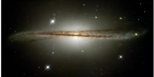
2.11. Warp of the spiral Galaxy ESO 510-13. Image Credit: NASA’s Hubble Space

Telescope . . . 18

2.12. The dust warp, in galactic coordinates, as traced by extinction from figure 8 of Marshall et al. (2006). Each panel describes the extinction at 1 kpc intervals from the nearest (top panel) to the further (bottom panel) distance. The black line indicates the position of the mid plane as given by the stellar warp formula

in Robin et al. (2003). . . 19

2.13. Schematic representation of the galactic structure. The flare is represented by the discontinuous line representing the thick disc which increases scale height

(15)

14 List of Figures

2.14. Figure from Minniti & Zoccali (2008). The velocity dispersion and mean veloc-ity as a function of the galactic longitude in the bulge component. Blue squares are K giants measured by Minniti (1996) and red crosses are M-giants measured by Rich et al. (2007) and which were corrected for the solar motion around the

Galaxy. . . 24

3.1. Figure 1 of Robin & Crézé (1986). Flowchart of the algorithm. . . 27

3.2. Scheme of the algorithm to compute the dynamical self-consistency. Ingre-dients for the equations are shown in italic, equations are shown in bold and

results from equations are underlined. . . 31

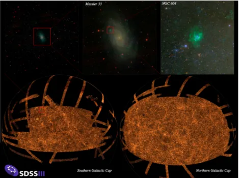
4.1. The SDSS sky coverage in the southern and northern Galactic cap. Image credit:

http://www.sdss.org/sdss-surveys/ . . . 38

4.2. The SEGUE in blue and SEGUE-2 in red sky coverage in Galactic coordinates.

Image credit: M. Strauss in http://www.sdss3.org/surveys/segue2.php . . . 39

4.3. The APOGEE sky coverage, from DR10, in Galactic coordinates. Image credit:

in http://www.sdss3.org/dr10/ . . . 40

4.4. The RAVE sky coverage where color are the stellar heliocentric radial

veloci-ties. Image credit: Axel Mellinger at http://www.rave-survey.aip.de/rave/pages/project/index.jsp

. . . 40

4.5. Simulation of the Gaia Galactic coverage. Image credit: X. Luri & the

DPAC-CU2 . . . 41

4.6. The Gaia Galactic coverage where the smaller and larger circles indicate the radius at which distances are accurate to 10% and the tangential velocities

ac-curate to 1 km s−1. Image credit: ESA/Lund . . . 42

4.7. The Gaia parallax errors. Top left panel: The G0V stars parallax error distri-bution without extinction. Top right panel: The G0V stars parallax error tribution with extinction. Bottom left panel: The K5III stars parallax error dis-tribution with extinction and no extinction. Bottom right panel: The Cepheids stars parallax error distribution with extinction and no extinction Image credit:

Lennart Lindegren . . . 42

4.8. Sky coverage of the observed targets in DR1 data release. Color indicates

the different target groups. MW: Milky Way fields;CL: Clusters; SD:

Standard Image credit: provided by Cambridge Astronomy Survey Unit (CASU)

-http://casu.ast.cam.ac.uk/gaiaeso/overview . . . 44

5.1. Difference between the SSPP temperature estimates and the corrected values as

a function of the SSPP temperature estimates for plate 2536 (l,b)=(70◦,14◦). . . 50

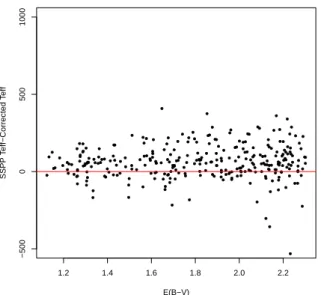
5.2. Difference between the SSPP temperature estimates and the corrected values as

a function of the extinction E(B-V) for plate 2555 (l,b)=(94◦,8◦). . . 50

6.1. Distribution in (l,b) of the simulated stars (red points) and observed ones (blue

points) for the field 2537. . . 51

6.2. The green points are the masked simulation and the red points are the full

(16)

List of Figures 15 6.3. Map of the Schlegel et al. (1998) extinction in the g band for the field 2536. We

can see in this figure regions where the extinction is homogeneous and low and

regions where the extinction is higher. . . 53

6.4. Map of the Schlegel et al. (1998) extinction in the g band for the field 2555. We can see in this figure regions where the extinction in g band can reach 8

magnitudes. . . 53

6.5. Map of the Drimmel & Spergel (2001) extinction model in the g band for the

field 2536. . . 53

6.6. Color magnitude diagram for the field 2536 (l,b)=(70◦,14◦). Density map along

with grey contours are observations. Black contours are simulations. . . 54

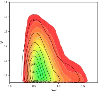
6.7. Color magnitude diagram for the field 2555 (l,b)=(94◦_,8◦_{). Density map along}

with grey contours are observations. Black contours are simulations. . . 55

6.8. Top panel: Total Av as a function of the distance from the Sun for field 2534

(l,b)=(50◦,14◦). Density contours are the total Av after correction and black

contours are before the correction. Bottom panel: Total Av distribution before

(red dashed line) and after correction (solid black line). . . 56

6.9. Total Avas a function of the distance from the Sun for field 2536 (l,b)=(70◦,14◦).

Density contours are the total Av after correction and black contours are before

the correction. Bottom panel: Total Avdistribution before (red dashed line) and

after correction (solid black line). . . 57

6.10. Total Avas a function of the distance from the Sun for field 2537 (l,b)=(110◦,10.5◦).

6.11. Total Avas a function of the distance from the Sun for field 2538 (l,b)=(110◦,16◦).

6.12. Total Avas a function of the distance from the Sun for field 2554 (l,b)=(94◦_,14◦_).

6.13. Total Avas a function of the distance from the Sun for field 2555 (l,b)=(94◦_,8◦_).

6.14. Total Av as a function of the distance from the Sun for field 2556 (l,b)=(94◦

,-8◦). Density contours are the total Av after correction and black contours are

before the correction. Bottom panel: Total Av distribution before (red dashed

line) and after correction (solid black line). . . 62

(17)

16 List of Figures

,-15◦_{). Density contours are the total Av} _{after correction and black contours are}

6.18. Color-magnitude diagram for region one of field 2555 (l,b)=(94◦_,8◦_{). Density}

map along with grey contours are observations. Black contours are simulations. 70

6.19. S/N as a function of the r magnitude for the plate 2668. Black points are

obser-vations and red points are simulations after applying the fit. . . 71

6.20. Parameter errors as a function of the S/N for plate 2699. Top left panel shows

the metallicity error, bottom left: effective temperature, top right: gravity,

bot-tom right: radial velocity. . . 71

7.1. Magnitude distribution for each individual region of the field 2536. The black

histograms are observations and the red histograms are simulations. . . 76

7.2. Color distribution for each individual region of the field 2536. The black

his-tograms are observations and the red hishis-tograms are simulations. . . 77

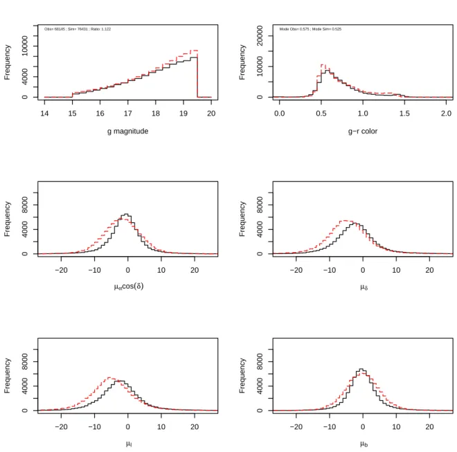
7.3. Magnitude, color (top panels) and proper motion distributions (middle and bot-tom panels) for field 2536. Black histograms are observations and the red

his-tograms are simulations. . . 79

7.4. Simulated magnitude, color (top panels) and proper motion distributions (bot-tom panels) separated by populations for field 2536. Thin disc stars: Black solid

line; Thick disc stars: Red dotted line; Halo stars: Blue dashed line. . . 81

7.6. Color distributions for each individual region of the field 2537. The black

7.8. Magnitude, color (top panels) and proper motion distributions (bottom panels) separated by populations for field 2537. Thin disc stars: Black solid line; Thick

disc stars: Red dotted line; Halo stars: Blue dashed line. . . 85

7.10. Color distributions for each individual region of the field 2537. The black

(18)

List of Figures 17 7.12. Magnitude, color (top panels) and proper motion distributions (bottom panels)

separated by populations for field 2538. Thin disc stars: Black solid line; Thick

7.28. Color distribution for each individual region of the field 2668. The black his-tograms are observations and the red hishis-tograms are simulations. . . 108 7.29. Color distribution for each individual region of the field 2678. The black

his-tograms are observations and the red hishis-tograms are simulations. . . 109 7.30. Color distribution for each individual region of the field 2681. The black

(19)

18 List of Figures

7.33. Magnitude, color (top panels) and proper motion distributions (middle and bot-tom panels) for field 2678. Black histograms are observations and the red his-tograms are simulations . . . 113 7.34. Magnitude, color (top panels) and proper motion distributions (bottom panels)

separated by populations for field 2678. Thin disc stars: Black solid line; Thick

7.37. Proper motion (in mas yr−1) measures of central tendency (Mean and Mode)

and of dispersion (Standard deviation) as a function of the galactic coordinates. black filled circles: mean of the observations; black open circles: mode of the observations; red filled triangles: mean of the simulations; red open triangles: mode of the simulations. Top panel: l and b components of the proper motion as a function of the galactic longitude. Bottom panel: l and b components of the proper motion as a function of the galactic latitude. . . 118 7.38. Mass distribution for the fields used to fit the IMF as given by the standard model.120

7.39. χ2_{as a function of the IMF slopes. . . 121}

7.40. χ2 for the magnitude distribution as a function of galactic longitude. The color

coding is galactic latitude. Circles are the original simulation and squares are model B of the revised version of the BGM. . . 123

7.41. χ2for the color distribution as a function of galactic longitude. The color coding

is galactic latitude. Circles are the original simulation and squares are model B of the revised version of the BGM. . . 124

7.42. χ2 for the color magnitude distribution as a function of galactic longitude. The

color coding is galactic latitude. Circles are the original simulation and squares are model B of the revised version of the BGM. . . 124 8.1. Distance from the plane as a function of the galactocentric distance for the

MSTO stars sample as given by the simulations. . . 126 8.2. Comparison of the spectrocopic observations and simulations for the bright

plate 2537, l = 110◦ and b = 10.5◦. Black points and lines are observations.

Simulations are in red. . . 127

8.3. Comparison of the spectrocopic observations and simulations for the faint plate

2545, l= 110◦and b= 10.5◦. Black points and lines are observations.

(20)

List of Figures 19

8.4. Mode of metallicities at different longitudes for the data and the standard model.

left panel are the bright plates and right panel are the faint plates. The observa-tions are in black and the simulaobserva-tions in red. The standard deviation is

repre-sented by the small bars. Squares are latitudes higher or equal to 14◦_{; Circles are}

latitudes between 8◦ and 10.5◦; Triangles are latitudes equal to -8◦; Diamonds

correspond to latitudes -12◦and -15◦. . . 129

8.5. Relation between effective temperature and absolute magnitude for the different

metallicity ranges. Top panel: [Fe/H] ≤ −0.5. Middle panel: −0.5 < [Fe/H] < 0.0. Bottom panel: [Fe/H] ≥ 0.0. Black points are simulations and the red line is the fit. . . 130

8.6. Difference between the new computed distance and the distance given by the

model as a function of the distance given by the model. The red line is an horizontal line that crosses the Y axis at zero. . . 131

8.7. Difference between distance estimate and the distance given by the model as a

function of the log(distance) given by the model. Density map and grey con-tours refer to our method and black concon-tours to Ivezi´c et al. (2008) method.

. . . 132 8.8. Correlations between parameters of the thick disc and old thin disc for case 1. . 135 8.9. Correlations between parameters for the thick disc and old thin disc fitting for

case 2 . . . 136

8.10. Mode of metallicities at different longitudes for the revised model (case 1). Left

panel are the bright plates and right panel are the faint plates. The observations are in black and the simulations in red. The standard deviation is represented

by the small bars. Squares are latitudes higher or equal to 14◦; Circles are

latitudes between 8◦ and 10.5◦; Triangles are latitudes equal to -8◦; Diamonds

are latitudes lower than -8◦_{. . . 138}

8.11. Effective temperature distributions for the original model (top panel) and

re-vised model (bottom plot) for plate 2538. Black lines are observations and red lines simulations. . . 140 8.12. Top panel: total extinction applied to the simulations as a function of the

dis-tance to the Sun. Density plot refers to the original simulation and black con-tours to the revised version. Bottom panel: Total extinction distribution applied

to the original model (black lines) and to the revised model (red lines). . . 142

8.13. Comparison of the spectrocopic observations and simulations for the bright plate 2536. . . 145 8.14. Comparison of the spectrocopic observations and simulations for the faint plate

2544. . . 145

9.1. Reddening from SFD maps and color distributions from GES data (black lines) and simulations (red lines) for field 074500 423000 (top panel) and field 154224

441200 (bottom panel). . . 154

9.2. Reddening from SFD maps and color distributions from GES data (black lines) and simulations (red lines) for field 155400 410000 (top panel) and field 160312 455359 (bottom panel). . . 155

(21)

20 List of Figures

9.3. Reddening from SFD maps and color distributions from GES data (black lines) and simulations (red lines) for field 170024 051200 (top panel) and field 173359 430000 (bottom panel). . . 156

9.4. Aitoff projection for the iDR2 fields selected for this analysis. . . 161

9.5. Spatial distribution for the F/G/K stars sample from GES as given by the

simu-lations. . . 161

9.6. Absolute magnitude as a function of the effective temperature for dwarf stars in

the three different metallicity ranges. From top to bottom the metallicity ranges

are [Fe/H] < −0.5, −0.5 ≤ [Fe/H] ≤ 0.0 and [Fe/H] > 0.0 respectively. . . . 163

9.7. Absolute magnitude as a function of the effective temperature for giants stars in

the three different metallicity ranges. From top to bottom the metallicity ranges

are [Fe/H] < −0.5, −0.5 ≤ [Fe/H] ≤ 0.0 and [Fe/H] > 0.0 respectively. . . . 164

9.8. Absolute magnitude as a function of the log g for subgiants stars in the two

different metallicity ranges. From top to bottom the metallicity ranges are

[Fe/H] ≤ −0.5 and [Fe/H] > −0.5 respectively. . . 165

9.9. Difference between distance estimate and the distance given by the model as a

function of the log(distance) (natural logarithm) given by the model. Density map and grey contours refer to our method. . . 166

9.10. Distribution of the differences between distance estimate and the distance given

by the model. . . 167 9.11. Metallicity distribution of the total GES sample from observations (grey lines)

and as given by simulations (Green lines). The different components as given

by the model are: black lines: Thin disc; red lines: Young thick disc; blue lines: Old thick disc; orange lines: Halo. . . 167 9.12. Comparison of the spectrocopic observations and simulations for a field at

l=229◦ and b=18◦. Left panels: Black lines are observations and simulations

are in red. The Poisson noise is represented by the small vertical bars. Right panels: Black lines are thin disc; red lines are young thick disc; blue lines are old thick disc; orange lines are halo. . . 168

9.13. Comparison of the spectrocopic observations and simulations for a field at l=97◦

and b=-61◦. Left panels: Black lines are observations and simulations are in red.

The Poisson noise is represented by the small vertical bars. Right panels: Black lines are thin disc; red lines are young thick disc; blue lines are old thick disc; orange lines are halo. . . 169

9.14. Effective temperature as a function of the J-K color for a field at l=97◦ _and

b=-61◦. Black points represent observations and red points simulations. . . 170

9.15. Distribution in (l,b) for all fields in GES sample. The color code represents the

difference between the mean observation and mean simulation for each field. . 174

9.16. Distribution in (l,b) for all fields in GES sample. The color code represents

the difference between mode of the observed distribution in metallicity and the

mode of the simulated distribution. . . 175 9.17. Correlations between parameters for the young thick disc and old thin disc

(22)

Table of figures 21

10.1. Galactocentric radius distribution for the F/G/K stars sample from GES (red

line) and MSTO from SEGUE (blue line) as given by the simulations. . . 180

10.2. Distance from the plane distribution for the F/G/K stars sample from GES (red

line) and MSTO from SEGUE (blue line) as given by the simulations. . . 180 10.3. Metallicity as a function of the galactocentric radius for the case 1 SEGUE

results (red lines) and GES SN metallicity and gradient results for the old thin disc. The continuous lines are the best values obtained and the dashed lines are

the combination of the different results taking into account the maximum and

minimum values for the errors. . . 181 10.4. Metallicity as a function of the galactocentric radius for the SEGUE results

(red lines) and GES SN metallicity and gradient results for the thick disc. The continuous lines are the best values obtained and the dashed lines are the

com-bination of the different results taking into account the maximum and minimum

(23)

(24)

23

List of Tables

2.1. Thin disc scale length and scale height values from the literature. . . 13

2.2. Thick disc scale length/height values from literature . . . 15

3.1. Table 1 from Robin et al. (2003). Defined initial mass function (IMF) and star

formation rate (SFR) for all the model components . . . 28

3.2. Table 4 from Robin et al. (2003). Age-velocity relations for the different

com-ponents of the model. . . 30

3.3. Table 1 from Robin et al. (2003). Metallicity distributions assumed in original simulations: Age, mean metallicity, radial metallicity gradient and dispersion

for each population. . . 32

3.4. SFR and IMF parameters in the standard and revised versions of the BGM. . . 33

3.5. Table 2 of Czekaj et al. (2014). Evolutionary tracks for the standard and revised

versions of the BGM . . . 34

3.6. Table 5 from Czekaj et al. (2014). Ingredients of the standard and revised

sim-ulations . . . 35

5.1. SEGUE survey plates used for the present analysis . . . 48

5.2. Photometric flags used . . . 48

5.3. Spectroscopic flags used . . . 49

6.2. Coefficients from the equation 6.2 for the correction to the DS extinction model.

The different lines in each field are the different regions in the field where the

program has been implemented. The regions were selected, from 1 to 9, firstly

from decreasing galactic latitude and then from increasing galactic longitude. . 65

6.1. Mean , mode, and dispersion of the distribution of the total extinction in V band

AV before (B) and after (A) correction for each field . . . 66

6.3. Coefficients from the equation 6.2 for the correction to the Marshall extinction

model. The different lines in each field are the different regions in the field were

the program has been implemented. The regions were selected as in table 6.2 . 69

6.4. Regression laws for S/N as a function of r magnitude. . . 72

6.5. Regression laws for radial velocity errors as function of g magnitude for each

plates. . . 73

7.1. Proper motions measures of central tendency (Mean and Mode) and of disper-sion (Standard deviation) for the l-component . . . 117

(25)

24 LIST OF TABLES

7.2. Proper motions measures of central tendency (Mean and Mode) and of disper-sion (Standard deviation) for the b-component . . . 119

7.3. χ2 values (magnitude(m), color(c) and color-magnitude(c-m)) along with

dis-persion (for the standard model). Last three lines show the sum of χ2_{values for}

all fields. . . 122

7.4. Deegres of freedom (df) for magnitude(m), color(c) and color-magnitude(c-m). 123

8.1. The number of stars of the thick disc/thin disc in the standard model in each

plate for the bright (b) and faint (f) plates after applying the selection sample.

The number of stars in each plate and the mode of the total extinction AV for

each distribution are also indicated. . . 126 8.2. Likelihood values for the spectroscopic parameters (MSTO stars) - original model128 8.3. Set of parameter range. The thick disc parameters have the subscript ’Thick’,

the old thin disc parameters have the subscript ’Old thin’ and the thin disc

pa-rameters have the subscript ’Thin disc’. . . 133

8.4. Thick disc and thin disc metallicity mean values, when fitting the thick disc and old thin disc.The SN subscript refers to solar neighbourhood value. . . 134 8.5. Thick disc metallicity mean values, when fitting the thick disc alone for case 2 . 137 8.6. Thick disc and thin disc metallicity mean set of parameters when fitting the

thick disc along with all thin disc - for case 2 . . . 137

8.7. Likelihood values for the spectroscopic parameters with the new sets of parameters139 8.8. Sum of the log likelihood values for all fields for the spectroscopic parameters

(MSTO stars) with the new set of parameters. . . 140

8.9. Sum of the likelihood values, for groups of fields of different longitudes, for the

spectroscopic parameters (MSTO stars) with the new set of parameters. . . 141 8.10. Thick disc and thin disc metallicity mean values, when fitting the thick disc

(two slopes) and old thin disc. Rchange is the galactocentric radius at which the

gradient of the thick disc changes. . . 141

8.11. Sum of the likelihood values, for different ages of the thick disc, for the

spec-troscopic parameters (MSTO stars) with the fitted parameters. . . 143

8.12. Thick disc and thin disc metallicity mean set of parameters - Fitting the old thin

disc for the model B of the revised version. . . 144

8.13. Thin disc metallicity distribution from the literature . . . 146 8.14. Thick disc metallicity distribution from the literature . . . 147 9.1. The value of the parameters used to compute the photometric errors in the

sim-ulation . . . 149

9.2. Mean reddening for each of the observed disc fields in GES . . . 150 9.3. Total extinction in each filter . . . 153 9.4. Number of stars, in the model, for the thin, young thick, old thick disc for each

field after applying the selection sample. The total number of stars in each field

(26)

List of tables 25 9.5. Set of parameters used to compute absolute magnitude from the relation with

effective temperature for dwarfs (logg > 4.5 dex) and giants (logg < 4.0 dex) and

with log g for subgiants (4.0 dex ≤ logg ≤ 4.5 dex). The selection in metallicity and log g is given in the first two columns respectively. . . 162

9.6. GES metallicity distribution . . . 171

9.7. Set of parameter range. The thick disc parameters have the subscript ’Thick’ and refer to the young thick disc. The subscript ’Old Thin’ refers to the older ages of the thin disc as explained in section 8.1.5. . . 175 9.8. Young thick disc and old thin disc metallicity mean values, when fitting the

(27)

(28)

1

Chapter 1 Motivation

The structure, formation and evolution of the Milky Way is still today under debate. Since Herschel and Kapteyn realized the importance of star counts the scientific community tried to create new and better observational surveys, but only in the last decades with the emergence of wide-field mosaic of CCD cameras it has been possible to create large complete catalogs. This large catalogs allowed the analysis and study of bright and faint magnitudes in vast areas of sky. This new large surveys create huge databases which allow a better exploration, star by star, of the Milky Way, as never done before and possibly not accessible for external galaxies in the near future. In this sense the Milky Way is a huge experimental laboratory from where we can obtain important information.

From the side of models and in particular stellar population synthesis models great effort

has been done to make possible to understand data and test different scenarios of formation

and evolution of the Milky Way. The existence of different models in the literature (Besançon

Galaxy Model (Robin et al. 2003), Trilegal (Girardi et al. 2005), GALFAST (Juri´c et al. 2008), Galaxia (Sharma et al. 2011)) is a proof of this work. The combination of the information taken

from the comparison of data with different models is a further step to understand the Milky Way

and realize our ”place” in the Universe.

The goal of this study is to use a stellar population synthesis model the Besançon Galaxy Model (Robin et al. 2003) to understand data and selection bias, study the stucture of the Milky Way and test scenarios of formation and evolution of our Galaxy. In particular this work uses photometric data to study the shape and spectrocopic data to study the metallicity, surface

grav-ity and effective temperature distributions in the different components of the Milky Way.

We organized the PhD manuscript in the following way: In the following chapter we

be-gin to describe how important was astronomy in the ancient world and the efforts done, by

different people, to have a better knowlodge of our place in the universe. We then depict the

most accepted scenario of the formation of the universe and we briefly describe the different

components of the Milky Way. In chapter 3 we introduce the BGM and describe the different

(29)

2 1. Motivation

future is presented in chapter 4. Chapter 5 describes the photometric and spectroscopic sam-ple used for this work. Chapter 6 explains how we proceed to obtain simulations, which we can compare with real observations, by masking, correcting extinction and applying errors. We

then explain the selection applied to obtain Main Sequence Turnoff Stars and K giants from the

SEGUE sample. Results for the photometric sample are given in chapter 7. We show quali-tative and quantiquali-tative comparisons for magnitude, color, color-magnitude and proper motion distributions. We describe how we tried to constrain the IMF and the comparisons with the re-vised version of the Besançon Galaxy Model. Chapter 8 present the spectroscopic comparisons between simulations and observations, discuss the metallicity distribution and describe how we

compute distances. This chapter also describes the ABC/MCMC method used to constrain the

radial metallicity gradients and metallicity distributions from the thin and thick disc and the

results. Chapter 9 describes the Gaia-ESO sample and F/G/K selection function, discuss the

metallicity distributions and describes how we computed distances along with the results from the analysis. In the last chapter we discuss and present conclusions from our results and give some perspectives for future work.

(30)

3

Chapter 2 Introduction

2.1 Astronomy in the antiquity

Astronomy dates to the antiquity, possibly to the pre-history and in the early times it was related to religion, mythology, calendars and general beliefs. The area of the science that studies these relations is called Archaeoastronomy, which is defined as the "anthropology of astronomy". Ob-jects in the sky were first identified as gods or spirits in early cultures. The early development of science can be studied by the analysis of these surviving indigenous traditions and from the structures that early civilizations left. There are few ancient astronomical sites around the world (e.g., France (Carnac), Germany, China, Scotland, Turkey, Malte, Egypt) that have been discov-ered. The ones in Malte, called Hagar Qim and Mnajdra, are among the oldest ones (3600 and 2500 BC) following a period of development (Cox 2008). The temple in Egypts Sahara desert (6500 - 6000 BC) is known as Nabta and it consists of five megalithic alignments constructed by

nomads1_{. The Gobeklitepe site in Turkey is probably the oldest known structure (c. 9600–7300}

BC)2_{. Why and by who it was constructed is still a mistery but its probable that it was a}

conse-quence of the development of that society and the need to understand the hereafter3. One of the

most popular structures (around 2800 BC), probably a astronomical observatory with religious functions, is Stonehenge in which one can follow in the aligned rocks, motions of the Sun and Moon (Lang 2006). Meanwhile, in Mesopotamia, the first lunar calendar has been developed and culminated in a continuous record of solar and lunar eclipses (Lang 2006). In China, as in other regions of the earth, the sky was also source of wonder and mystery, which lead to an in-terest in observations. The Chinese, as the Babylonian, Egyptians, Hindus, Mayas, Celts among others, were among the first to record the sighting of a comet, the eclipse of the Moon, eclipse

1_URL:

http://www.colorado.edu/news/releases/1998/03/31/oldest-astronomical-megalith-alignment-discovered-southern-egypt-science

2_{URL: http:}_{//www.gobeklitepe.info/}

3_{David Lewis-Williams et David Pearce, « An Accidental revolution? Early Neolithic religion and economic}

(31)

4 2. Introduction

of the Sun and create a calendar with 12 months of 30 days each4 5_{. First predictions were made}

in ancient Greece when Thales of Miletus (624 - 547 BC) estimated correctly a solar eclipse (around 585 BC) (Lang 2006). In this epoch the Greek civilization contributed for countless developments in astronomy as the planets constitution, shape, movement and placement. In 530 BC Pythagoras (572-479 BC) proposes a spherical shape for the earth, planets and Sun later modelized by Eudoxus of Cnidus (408-355 BC) which constructed a geocentric model of the solar system and stated that movements of stars in the sky where due to the Earth’s rotation

6_{. Later, Aristarchos of Samos (320-250) proposed that the Sun instead of the Earth is in the}

center of the solar system. The Heliocentric model was later celebrated by Nicolaus Copernicus (1473-1543) in the text De Revolutionibus and Johannes Kepler (1617–1621) text Astronomia nova. In 350 BC Aristotle (384-322 BC) proved that the Earth as a spherical shape as already proposed by Pythagoras. Among one of the important contributions, due to the Greeks, is the first known star catalog of 850 stars (129 BC), made by the Greek astronomer Hipparchus (190-120 BC), later celebrated by Ptolemy (87-165). Meanwhile, astronomers began to understand

that the universe is an hierarchical composition of different structures also called islands. In

particular a milky patch of sky that rings the Earth, known in latin by Via Lactea which trans-lates to road of milk, was of particular interest. This name was given due to the pale band of light formed by stars, gas and dust in the galactic plane as seen from Earth.

Eighteen-century astronomers were the first to realize that we make part of an enormous disk of stars, gas and dust which appears as a band around the sky due to the edge-on view from inside this disc. The Sun location in this structure was one of the first questions that arose. The first attempt to deduce the Sun location has been made by William Herschel (1738-1822). Around 1785 the first systematic survey of the sky was made by Herschel and his sister Caroline (1750-1848) in an attempt to deduce the structure of the Milky Way. The technique of star counts was being used for the first time and it was done for 683 regions of the sky. He reasoned that towards the galactic center the density of stars, compared with the average density, should be higher and towards the edge of the Galaxy should be lower. Figure 2.1 shows the map constructed by William and Caroline Herschel. They noticed that the lower density regions were outside the Milky Way which means that the shape is a disc. Because the density of stars was the same in all directions he concluded wrongly that the Sun is in the center of the Galaxy.

Later Jacobus Kapteyn (1851-1922) used observations fairly well represented, at least up to

galactic lat. 70◦ (Kapteyn 1922) that he called ’Selected Areas‘ to produce a catalog which he

used to construct a higher precision map of the Milky Way than Herschel. Kapteyn introduced, in the catalog, motion, density, and luminosity to the Herschel’s star counts map. Figure 2.2 shows the Kapteyn’s map of the Milky Way.

The map shows that the Milky Way has a flattened disc with a radius of 8.0 kpc. The Sun is represented by a large circle around 2.0 kpc. Both, Herschel and Kapteyn, agree that the Milky Way is a flat structure with the Sun placed near the center but nevertheless the enormous

4_{URL: http:}_{//casswww.ucsd.edu/archive/public/tutorial/History.html} 5_{URL: http:}_{//image.gsfc.nasa.gov/poetry/ask/a11846.html}

(32)

2.2. Galaxy formation in a Λ cold dark matter scenario 5

Figure 2.1: Herschel map of the Milky Way. The darker black point near the center of the map is the Sun position. Source: On the Construction of the Heavens. By William Herschel, Esq. F. R. S. Philosophical Transactions of the Royal Society of London, Vol. 75. (1785), pp. 213-266.

Figure 2.2: Kapteyn’s map of the Galaxy. Source: Kapteyn (1922)

effort made by both the results were skewed because the authors were not aware of the strong

extinction effect. In effect they were looking only to the nearest stars and had no idea about

the actual size of the Galaxy. Later Harlow Shapley (1885-1972) analysing globular clusters RR Lyrae variables, computed distances and charted the distribution of globular clusters. He discovered that the Milky Way was at least two times larger than supposed by Kapteyn and that the globular clusters and stars in general orbited a common center far from the Sun in the direction of the Sagittarius constellation. In 1924, Edwin Hubble (1889-1953) at Mount Wilson made observations of Cepheids in the Andromeda Nebula and realized that it was too distant to be part of the Milky Way. It was demonstrated that the Milky Way is just one Galaxy among others in a large scale structure. This epoch defines the beginning of cosmology as a scientific area and of particular interest the formation of Galaxy’s in a large scale structure as the Universe.

2.2 Galaxy formation in a

Λ cold dark matter scenario

The Λ cold dark matter scenario (hereafter ΛCDM) (e.g. Blumenthal et al. (1984), Springel

et al. (2006), and references therein) is the most accepted scenario for the formation of the Universe. The haloes of CDM were formed from the density fluctuations after de Big Bang and its imprints remain visible in the Cosmic Microwave Background (hereafter CMB). Figure 2.3 show how the imprints from the early universe and specially the Baryon Acoustic Oscillations (BAO) are related with the large scale structure (Boughn & Crittenden 2004; Springel et al. 2006).

(33)

6 2. Introduction

Figure 2.3: An illustration of the concept of baryon acoustic oscillations, which are imprinted in the early universe and can still be seen today in Galaxy surveys like the Baryon Oscillation

Spectroscopic Survey (BOSS; Schlegel et al. 2009). Image Credit: Chris Blake and Sam

Moorfield in https://www.sdss3.org/surveys/boss.php

The visible structures of the universe are made of baryonic mass accreted in these haloes. At around Z ∼ 10 star formation begins which drives gas out from the protogalactic dark matter mini-halos (e.g., Springel & Hernquist 2003; Schultz et al. 2014). These first stars will belong to the stellar halo and are among the oldest stars in galaxies. As the time goes the hot gas, around the Galaxy, that is cooling and falling into the plane, gives rise to a rotating disc which at the beginning probably increases the Star Formation Rate. This scenario is well in agreement with large scale observations as the CMB provided by WMAP (Wilkinson Microwave Anisotropy Probe) (Spergel et al. 2007) but there are numerous predictions, at the scale of the Milky, which are not observed. We will briefly review few of them.

• Structure of the inner dark halo - A core or cusp shape?: The cuspy-halo problem arose in the early 1990s, when the first N-body simulations became available (Dubinski & Carlberg 1991; Navarro et al. 1996, 1997). The simulations were better described by a steep power-law mass density distribution, like a cuspy distribution (Dubinski & Carlberg 1991), instead of the observed core like behavior (see; de Blok 2010, for a general review). • Number of predicted satellites (MSP): From predictions, a Galaxy as the Milky Way,

should have around 500 satellites with masses higher than 108 M (Moore et al. 1999).

These objects were not still found in large numbers either in HI or visible studies. Lately there are some very faint satellite galaxies and dwarf spheroidal satellite galaxies which are dominated by dark matter being discovered (Mateo 1998; The Fermi-LAT Collabora-tion et al. 2013) but they are unlikely to arrive to the hundred. The large predicted number of satellites should leave a large number of debris of accreted satellites in the stellar disk and halo. An example of the active ongoing accretion history are stellar streams (Newberg et al. 2002; Belokurov et al. 2007) which were minor satellites disrupted by tidal forces.

(34)

2.3. Structure of the Milky Way 7 Several studies (Toth & Ostriker 1992; Kormendy & Fisher 2005; Kautsch et al. 2006; Stewart et al. 2008) showed that a large accretion activity, in particular the possibility of the interaction with a large merger, may be in disagreement with the presence of a strong disc as the Milky Way disc while Bournaud & Elmegreen (2009) and Dekel et al. (2009) predict the stabilization (we mean in terms of its existence) of the disc after z ∼ 1.

• Forming disks with small bulges in ΛCDM: In the ΛCDM scenario the formation of

bulges is critical because its very difficult to generate galaxies without or with a very

small bulge (van den Bosch 2001). Some recent advances have been made in this field. Brook et al. (2011) showed that in order to generate bulgeless disc galaxies the Galaxy has to expell large amounts of low angular momentum gas during merger events at early epochs which modifies the shape of the angular momentum distribution of baryons, from the original one given by the parent dark matter haloes, allowing the creation of smaller bulges.

• Angular momentum catastrophe (AMC): The lack of angular momentum of baryons (around 10%), for SPH simulations of galaxies, in comparison with real galaxies and the predicted smaller disc sizes in comparison with real discs is called “angular momentum catastrophe” (Navarro & Benz 1991; Navarro & Steinmetz 1997; Sommer-Larsen et al. 1999; Navarro & Steinmetz 2000).

• The Too Big to Fail problem: The Too Big to Fail problem (hereafter TBTF) is a par-ticular case of the MSP. In simulations,where just Dark Matter is taken in account the central densities in subhalos are larger than the ones observed (Del Popolo et al. 2014).

Several individual solutions have been proposed for the listed problems. More recently Del Popolo et al. (2014), using the Del Popolo (2009) model, showed that the jointly small

scale problems (cusp/core problem, MSP, TBTF problem, and the AMC) of the CDM scenario

may be reconciled with observations by taking a semi-analytical model which takes in account,

for the first time, the effect of ordered and random angular momentum, adiabatic contraction,

dynamical friction, and the exchange of angular momentum between baryons and Dark Matter Del Popolo et al. (2014).

2.3 Structure of the Milky Way

The Milky Way is a barred spiral Galaxy composed of a disc (thin and thick disc), a bulge and a halo (stellar and dark matter halo) as showed in figure 2.4 (Buser 2000). The formation of the protogalaxy is still under debate but the most accepted scenario is one where the formation is hierarchical i.e. the halo is formed by satellite Galaxy accretion (Blumenthal et al. 1984; Springel et al. 2006), and references therein) (see section 2.2). The Milky Way has of the

order of 1.0 − 2.0 × 1011 stars and the dark matter halo can extend at least to 100 kpc possibly

being in contact with other galaxies dark matter haloes like Andromeda.Last measurements of

(35)

8 2. Introduction

Figure 2.4: The Milky Way edge-on view showing the different components of the Milky Way

with the Sun position indicated. Image Credit: R. Buser. Hurt

(6.43 ± 0.63) × 1010M (McMillan 2011). The disc is not axisymmetric and the spiral arms

nature, long-lived or transient, is still under debate. In recent past the disc was thought to be composed by two main arms (Perseus and Scutum-Centaurus arms) (Grabelsky et al. 1988), but the quantity of recent works indicating that the Milky Way have instead 4 arms increased to around 80% of the published papers on this question (Vallée 2014). The possible existence of 4 arms was first given from the analysis of HII regions (Georgelin & Georgelin 1976) and more recently Vallee (2014) from a meta-analysis. The Sun is located in the range of 8.0 kpc (Reid 1993; Brunthaler et al. 2011) to 8.5 kpc (IAU value) from the galactic center and 15 pc above the galactic plane (Hammersley et al. 1995; Freudenreich 1998; Drimmel & Spergel 2001) as showed in figure 2.5. The artist also places the Galactic bar and a hypothetical second bar.

The edge of the disc is detected at a galactocentric distance of about 14 kpc in some analysis (Robin et al. 1992; Ruphy et al. 1996; Minniti et al. 2011) but it is a scenario still under debate (Carraro 2014).

The nature and formation of the bulge of the Milky Way are still under debate. The bulge

is elongated as a bar (Stanek et al. 1994; Dwek et al. 1995) and is inclined by an angle (∼25◦)

with respect to the line of sight. The side nearest to us is at positive galactic longitudes and the boxy bulges, as in our Galaxy, are associated with bars formed from bar-buckling instability of the disc (Saha & Gerhard 2013).

Galaxys have also a large content of dark matter which was first proposed due to the Galaxy rotation problem. The discrepancy between theoretical predictions, assuming that the total mass is the sum of all the luminous components masses, and observations at large galactocentric radius lead to conclude the existence of a not luminous mass which was called dark matter (Rubin et al. 1978, 1980). Figure 2.6 shows the predicted and observed rotation curve for the M33 Galaxy. The discrepancy between the expected rotation from the visible matter and the observed one appears at larger radii.

(36)

2.3. Structure of the Milky Way 9

Figure 2.5: The Milky Way face-on view with the Sun position indicated. Artist’s impression

of the Milky Way. Image Credit: NASA/JPL-Caltech/ESO/R.

Figure 2.6: The observed and predicted rotation curve of the Galaxy M33. Image credit:

(37)

10 2. Introduction

Figure 2.7: The predicted rotation curve from the self-consistent model of the Milky Way Robin et al. (2003). The contributions from each component of the Milky Way is also visible.

The observations are from Caldwell & Ostriker (1981)

2.4 Galactic populations

Working at Mount Wilson Observatory outside of Los Angeles and taking advantage of the Los Angeles blackouts during the second world war Walter Baade (1893–1960) resolved for the first time Andromeda Galaxy and both companions Messier 32 and NGC 205 (Baade 1944).

Baade found that the stars fall into two different groups which he called population I and

popu-lation II and concluded that popupopu-lation I stars, which are found in the solar neighbourhood, are mainly younger stars and can be found in sub-structures as open clusters while population II are found mainly in globular clusters. It is in 1957 in the Vatican conference that the definition of the two population was set. Stars from population I are younger more metal rich stars and seem to be constrained into the disc. Population II is composed of old metal poor stars that

are homogeneously distributed in a sphere. The dynamics from both populations is also di

ffer-ent as population I have circular orbits with small eccffer-entricity and confined to the disc while population II stars have highly eccentric and inclined orbits (Figure 2.8). Later a population III was proposed for even older stars probably connected with the reionization epoch. The term stellar populations has evolved with time and nowadays, instead of classify stellar classes as decreasing metallicity and increase age (Ivezi´c et al. 2012), the term stellar population means

a collection of stars which has a common spatial, kinematic, chemical, luminosity, and/or age

(38)

2.5. Disc of the Milky Way 11

Figure 2.8: A scheme showing the orbits of population I and II.Image credit: Nick Strobel at www.astronomynotes.com.

Figure 2.9: Schematic representation of a disc structure. Artist’s impression of the Milky Way.

Image Credit: Amanda Smith, IoA graphics officer

2.5 Disc of the Milky Way

The disc contains most of the dust, gas and stars of the Milky Way. The disc is flat, supported by rotation and shows a spiral structure delineated by gas and young stars. The stellar, gas and dust orbits lie in the plane of the Galaxy defined by the disc. Stars in the disc show a large range of ages and the mean peculiar motions of gas, dust and stars are small. The disc is the component of the Milky Way where the density of stars is higher. The stellar disc has a diameter of around 30 kpc and the Sun is around 8 kpc from the galactic center and 15 pc above the

galactic plane. The total mass of the disc is around 6.5 × 1010M(e.g., Flynn et al. 2006; Sofue

et al. 2009; McMillan 2011). The local dark matter density is around 0.40 ± 0.04 GeV cm−3

(McMillan 2011). The existence of two components in the disc is still under debate although it is generally accepted that there is a younger component formed essencially of population I stars called the thin disc and an older component, the thick disc, composed essencially of an intermediate population between population I and II stars. Figure 2.9 shows the decomposition

of the disc into two different components as explained above. This decomposition is also seen