HAL Id: hal-00328442
https://hal.archives-ouvertes.fr/hal-00328442
Submitted on 20 Jun 2006
HAL is a multi-disciplinary open access
archive for the deposit and dissemination of
sci-entific research documents, whether they are
pub-lished or not. The documents may come from
teaching and research institutions in France or
abroad, or from public or private research centers.
L’archive ouverte pluridisciplinaire HAL, est
destinée au dépôt et à la diffusion de documents
scientifiques de niveau recherche, publiés ou non,
émanant des établissements d’enseignement et de
recherche français ou étrangers, des laboratoires
publics ou privés.
global biogenic volatile organic compound emissions
J. Lathière, D. A. Hauglustaine, A. D. Friend, N. de Noblet-Ducoudré, N.
Viovy, G. A. Folberth
To cite this version:
J. Lathière, D. A. Hauglustaine, A. D. Friend, N. de Noblet-Ducoudré, N. Viovy, et al.. Impact of
climate variability and land use changes on global biogenic volatile organic compound emissions.
Atmo-spheric Chemistry and Physics, European Geosciences Union, 2006, 6 (8), pp.2129-2146.
�10.5194/acp-6-2129-2006�. �hal-00328442�
www.atmos-chem-phys.net/6/2129/2006/ © Author(s) 2006. This work is licensed under a Creative Commons License.
Chemistry
and Physics
Impact of climate variability and land use changes on global
biogenic volatile organic compound emissions
J. Lathi`ere1, D. A. Hauglustaine1, A. D. Friend1, N. De Noblet-Ducoudr´e1, N. Viovy1, and G. A. Folberth2 1Laboratoire des Sciences du Climat et de l’Environnement (LSCE), Gif-sur-Yvette, France
2School of Earth and Ocean Sciences (SEOS), University of Victoria, Victoria, Canada
Received: 19 July 2005 – Published in Atmos. Chem. Phys. Discuss.: 25 October 2005 Revised: 28 February 2006 – Accepted: 22 April 2006 – Published: 20 June 2006
Abstract. A biogenic emissions scheme has been
incorpo-rated in the global dynamic vegetation model ORCHIDEE (Organizing Carbon and Hydrology in Dynamic Ecosys-tEms) in order to calculate global biogenic emissions of isoprene, monoterpenes, methanol, acetone, acetaldehyde, formaldehyde and formic and acetic acids. Important param-eters such as the leaf area index are fully determined by the global vegetation model and the influences of light extinc-tion (for isoprene emissions) and leaf age (for isoprene and methanol emissions) are also taken into account. We study the interannual variability of biogenic emissions using the satellite-based climate forcing ISLSCP-II as well as relevant CO2 atmospheric levels, for the 1983–1995 period. Mean
global emissions of 460 TgC/yr for isoprene, 117 TgC/yr for monoterpenes, 106 TgC/yr for methanol and 42 TgC/yr for acetone are predicted. The mean global emission of all bio-genic compounds is 752±16 TgC/yr with extremes ranging from 717 TgC/yr in 1986 to 778 TgC/yr in 1995, that is a 8.5% increase between both. This variability differs signif-icantly from one region to another and among the regions studied, biogenic emissions anomalies were the most vari-able in Europe and the least varivari-able in Indonesia (isoprene and monoterpenes) and North America (methanol). Two sce-narios of land use changes are considered using the 1983 cli-mate and atmospheric CO2 conditions, to study the
sensi-tivity of biogenic emissions to vegetation alteration, namely tropical deforestation and European afforestation. Global biogenic emissions are highly affected by tropical deforesta-tion, with a 29% decrease in isoprene emission and a 22% increase in methanol emission. Global emissions are not sig-nificantly affected by European afforestation, but on a Euro-pean scale, total biogenic VOCs emissions increase by 54%.
Correspondence to: J. Lathi`ere
(juliette.lathiere@cea.fr)
1 Introduction
The terrestrial biosphere is a major source of natural volatile organic compounds (VOCs). Isoprene and monoterpenes dominate biogenic emissions but other highly reactive chem-ical species, such as methanol, acetone, aldehydes and or-ganic acids, are now also recognized to be emitted by the terrestrial vegetation at significant levels, as shown by sev-eral measurement campaigns (Kirstine et al., 1998; Schade and Goldstein, 2001; Villanueva-Fierro et al., 2004). Global VOCs emissions by the vegetation are 1150 TgC/yr (Guen-ther et al., 1995), corresponding to nearly 90% of global VOC emissions at the surface (including anthropogenic emissions).
Those biogenic compounds play a crucial role in tropo-spheric chemistry, from local to global scales, inducing in-creased or dein-creased ozone formation, depending on NOx
levels (Fehsenfeld et al., 1992; Thunis and Cuvelier, 2000; Pun et al., 2002). Recently, Barket al. (2004) showed that isoprene photooxidation results in maximum ozone produc-tion rates for NOx concentrations in the range of about 1–
10 ppbv, a typical level of anthropogenically influenced ru-ral environments. Wang and Shallcross (2000) used a global land-surface and chemistry-transport model to show that the inclusion of isoprene emissions, estimated at 530 TgC/yr for present day conditions, has a significant impact on ozone and oxidation products, such as peroxyacetyl nitrate (PAN), in both hemispheres. Their analysis indicated that the response of ozone to isoprene emissions was predominantly governed by the spatial and temporal variations in terrestrial vegeta-tion, with a simulated ozone increase of about 4 ppbv over the oceans and about 8–12 ppbv over mid-latitude continental ar-eas. Sanderson et al. (2003) illustrated the impact of climate change on both isoprene emissions and ozone levels. Based on a global isoprene emission increase from 484 TgC/yr for the 1990s to 615 TgC/yr for the 2090s, as a result of climate and vegetation distribution changes, the authors calculated an
ozone increase by 10–20 ppbv in some locations. They also noted that the changes in ozone levels were closely linked to changes in isoprene surface fluxes in regions such as the east-ern U.S. or southeast-ern China. However, this effect was much less marked over the Amazon region and Africa because of lower levels of nitrogen oxides.
In addition to their importance for gas phase chemistry, the involvement of biogenic VOCs in tropospheric aerosols formation, first suggested by Went (1960), has lately been demonstrated (Griffin et al., 1999), and enforces the impor-tance of taking into account biogenic VOC in both tropo-spheric gas phase reactions and particulate formation. As-suming an aerosol yield from the oxidation of biogenic VOC other than isoprene (monoterpenes and other VOC) between 5% and 40%, Andreae and Crutzen (1997) suggested that the secondary organic aerosols (SOA) formation could range between 30 and 270 Tg of organic matter per year. More recently, Tsigaridis and Kanakidou (2003) estimated, using a global chemistry-transport model, that the production of SOA from biogenic VOC might range from 2.5 to 44.5 Tg/yr Furthermore, Kanakidou et al. (2000) estimated that the pro-duction of SOA from biogenic VOCs increased from 17– 28 Tg/yr in preindustrial times to 61–79 Tg/yr for present day conditions, which was attributed to an increase in ozone and primary organic aerosol from anthropogenic sources. In ad-dition to the recognized role of monoterpenes SOA forma-tion (Kavouras et al., 1999; Sotiropoulou et al., 2004), recent studies (Limbeck et al., 2003; Claeys et al., 2004) also sug-gest the importance of isoprene in aerosol formation, leading to 2 Tg of organic matter per year (Claeys et al., 2004).
Key parameters, such as environmental conditions (mainly temperature and radiation), vegetation type and foliar area, constrain biogenic emissions, thus making them very sensi-tive to climate and land use changes. In addition, vegeta-tion is not only influenced by climate change but also human activity and development, such as urbanization and agricul-ture expansion. Mainly initiated by Guenther et al. (1995), global biogenic emissions modeling now benefits from dy-namic vegetation models, allowing the calculation of bio-genic emissions for the present day, as well as studying their possible future evolution in response to vegetation and cli-mate changes (Levis et al., 2003; Sanderson et al., 2003; Naik et al., 2004; Lathi`ere et al., 2005). The History Database of the Global Environment (HYDE), developed by Goldewijk (2001) to estimate global land use changes over the past 300 years (1700–1990), based on historical statistical inventories and spatial analysis techniques, sug-gests a global increase of cropland area from 265×106ha in 1700 to 1471×106ha in 1990, and a more than six fold increase of pasture area from 524×106to 3451×106ha. Im-portant regional differences are found: most of the land use change occurred during the 19th century in temperate re-gions of Canada, the United States, Russia and Oceania, whereas in most of the tropical regions, the largest rate of land use conversion occurred at the end of the last century. A
study of the impact of deforestation in Amazonia on tropo-spheric chemistry (Ganzeveld and Lelieveld, 2004), replac-ing tropical rainforest by pasture, predicted a large decrease in maximum isoprene emission fluxes, from 12×1015 to 1.2×10¹⁵molecules m−2s−1 (=11.9×10⁻¹¹kgC/m2/s) due to a decrease in the isoprene emission factor and in the foliar density. Furthermore, a large reduction in the diurnal ozone deposition velocity and an increase of nocturnal soil deposi-tion were predicted Steiner et al. (2002) estimated that in East Asia, the human-induced land-cover changes, characterized by the conversion of about 30% of the land area from forests to cropland, led to a decrease of 30% in isoprene and 40% in monoterpenes annual emissions. On the other hand, forest restoration efforts are done in some regions such as boreal and temperate zones of North America and western Europe, leading to an increase in forest cover (Stanturf and Madsen, 2002), which could also affect significantly biogenic emis-sion levels and tropospheric chemistry.
The main goal of our work is to study the sensitivity of global biogenic emissions to, first, climate and atmospheric CO2interannual variability and, second, to vegetation
distri-bution changes. We have incorporated a biogenic emission scheme in the dynamic global vegetation model ORCHIDEE to calculate not only isoprene and monoterpenes emissions but also methanol, acetone, acetaldehyde, formaldehyde, formic and acetic acids.
In Sect. 2 of this paper, we describe the interactive bio-genic emission and vegetation model used in our study, as well as details of the simulations. Global mean estimates for the 1983–1995 period are given in Sect. 3 and compared to the results of other studies. Analysis of the impact of climate and CO2 interannual variability from 1983 to 1995 on the
simulated biogenic VOC emissions is presented in Sect. 4. Finally, two scenarios of land use change, tropical deforesta-tion and European afforestadeforesta-tion, are considered in Sect. 5 to analyse the sensitivity of biogenic emissions to the vegeta-tion distribuvegeta-tion alteravegeta-tion.
2 The interactive biogenic emission and vegetation model
2.1 General description
A biogenic emission scheme, based on Guenther et al. (1995) parameterizations, has been incorporated into the dynamic global vegetation model ORCHIDEE (Or-ganizing Carbon and Hydrology in Dynamic Ecosys-tEms) (Krinner et al., 2005). This terrestrial biosphere model consists of the surface-vegetation-atmosphere transfer scheme SECHIBA (Sch´ematisation des ´echanges hydriques `a l’interface biosphere-atmosph`ere), (Ducoudr´e et al., 1993; De Rosnay and Polcher, 1998) and of the carbon module STOMATE (Saclay-Toulouse-Orsay Model for the Analy-sis of Terrestrial Ecosystems), which includes the dynamic
vegetation component of the LPJ (Lund-Potsdam-Jena) dy-namic model (Sitch et al., 2003).
SECHIBA calculates processes characterized by short time-scales, ranging from a few minutes to hours, such as energy and water exchanges between the atmosphere and the terrestrial biosphere, photosynthesis, as well as the soil wa-ter budget. SECHIBA has a time step of 30 min in order to simulate the diurnal cycle of the terrestrial biosphere. STO-MATE treats daily processes such as carbon allocation, lit-ter decomposition, soil carbon dynamics, phenology, mainte-nance and growth respiration. Important parameterizations, allowing the dynamic simulation of vegetation distribution, have been taken from the global model LPJ: processes such as fire, sapling establishment, light competition, tree mor-tality and climatic criteria for the introduction and elimina-tion of plant funcelimina-tional types are integrated into ORCHIDEE, with a time step of one year.
In the ORCHIDEE model, the land surface is described as a mosaic of twelve plant functional types (PFTs) and bare soil (Fig. 1). The definition of PFT is based on ecologi-cal parameters such as plant physiognomy (tree or grass), leaves (needleleaf or broadleaf), phenology (evergreen, sum-mergreen or raingreen) and photosynthesis type for crops and grasses (C3or C4). Relevant biophysical and
biogeochemi-cal parameters are prescribed for each PFT (Krinner et al., 2005). This distinction is of great importance since the na-ture and the amount of the biogenic VOCs emitted are very different from one vegetation type to another. In the current version of ORCHIDEE there is no explicit terrestrial nitro-gen cycle. However, nitronitro-gen is implicitly taken into account in the photosynthesis and carbon allocation calculations. For carbon allocation, a nitrogen limitation is parameterized as a function of monthly soil moisture and temperature, because nitrogen availability of a plant depends on microbial activity in soil, and thus on soil moisture and temperature. Photosyn-thesis is parameterized as an exponential function decreas-ing with canopy depth, with an asymptotic minimum limit of 30% of the maximum efficiency, to take into account ver-tical variation of photosynthetic capacity based on leaf ni-trogen content. Leaf onset and senescence are calculated, depending on the PFT, by applying warmth and/or moisture stress criteria to the meteorological conditions. Carbon allo-cation to leaves, and to other compartments such as roots and sap wood, depends on external constraints such as tempera-ture, moisture or light. The more stress a tissue will suffer, the more carbon it receives. In addition, a maximum leaf area index (LAI) value, above which no carbon will be allo-cated to leaves, is prescribed for each PFT: 7 m2/m2for trop-ical trees, 5 m2/m2for temperate trees, 3 and 4.5 m2/m2for boreal forests, 2.5 m2/m2for grasses and 5 m2/m2for crops (Fig. 1). The leaf photosynthetic efficiency varies during its life cycle: small when the leaf is young, it increases quickly with the leaf age up to a maximum value, lasting until the leaf age equals half its critical value, and then decreases. To take into account this feature, a leaf age structure has been
imple-No. PFT Description Maximum LAI Critical leaf age (m2/m2) (days) 1 Bare soil
2 Tropical broadleaf ever-green tree
7 730
3 Tropical broadleaf rain-green tree
7 180
4 Temperate needleleaf ev-ergreen tree
5 910
5 Temperate broadleaf ev-ergreen tree
5 730
6 Temperate broadleaf summergreen tree
5 180
7 Boreal needleleaf ever-green tree
4.5 910 8 Boreal broadleaf
sum-mergreen tree
4.5 180 9 Boreal needleleaf
sum-mergreen tree 3 180 10 C3 Grass 2.5 120 11 C4 Grass 2.5 120 12 C3 Agriculture 5 120 13 C4 Agriculture 5 120
Fig. 1. Dominant plant functional types (PFTs) in ORCHIDEE,
cor-responding maximum leaf area index (LAI in m2/m2)and critical
leaf age (in days).
mented in the ORCHIDEE model. In the current model ver-sion, 4 leaf age classes are considered, each corresponding to various leaf efficiency regimes and of equal duration (=crit-ical leaf age/number of leaf age classes). The crit(=crit-ical leaf age is 910 days for needleleaf evergreen trees, 730 days for broadleaf evergreen trees, 180 days for raingreen and sum-mergreen trees and 120 days for grasses and crops. This fea-ture is critical in accounting for the leaf age influence on bio-genic emissions (MacDonald and Fall, 1993; Guenther et al., 2000).
ORCHIDEE can either be forced by archived climate fields or driven by a general circulation model and can run in various modes, depending on the activated model compo-nents. For instance, the natural PFT distribution can either be
Fig. 2. Monthly mean Leaf Area Index (LAI, m2/m2)calculated by ORCHIDEE for January and July.
prescribed from an inventory (static mode, LPJ not activated) or entirely simulated by the model (dynamic mode, LPJ acti-vated), depending on climate conditions. The fraction of the grid box occupied by agricultural PFTs is always prescribed so that crop extent is not affected by the dynamic vegetation change. The atmospheric CO2levels influence
photosynthe-sis, and consequently, the LAI, and can thus indirectly affect VOC biogenic emissions. It is thus really important to con-sider the relevant CO2atmospheric level for each year and
take into account its evolution throughout the period anal-ysed.
Validation studies showed that the ORCHIDEE model ac-curately simulates water, energy and carbon exchanges, as well as vegetation processes on short and long time-scales. A more detailed description of the ORCHIDEE model and its validation is presented in Krinner et al. (2005), and its good skills for interannual variability have been illustrated by Ciais et al. (2005).
2.2 Biogenic emission model
In addition to isoprene and monoterpenes, we also explic-itly estimate the emissions of methanol, acetone, acetalde-hyde, formaldeacetalde-hyde, formic and acetic acids, which are usu-ally considered as a family of compounds and estimated as bulk emissions. VOC biogenic emissions are calculated ev-ery 30 minutes, based on the Guenther et al. (1995) param-eterizations, and integrate additional feature such as the leaf age influence on isoprene and methanol emissions.
The generic formula is:
F = LAI × s × Ef ×CT ×CL×La (1)
where F is the flux of the considered biogenic species, given in µgC/m2/h and LAI the leaf area index in m2/m2, calcu-lated at each time step by the model (Fig. 2). The specific leaf weight s in gdm/m2(dm: dry matter) is prescribed in OR-CHIDEE depending on the considered PFT. Ef is the
emis-sion factor in µgC/gdm/h prescribed for each PFT and bio-genic species (Table 1). Isoprene, and monoterpenes emis-sion factors are based on Guenther et al. (1995) and adapted to the PFTs considered in ORCHIDEE. For methanol, we use emission factors from Guenther et al. (2000) and Mac-Donald and Fall (1993), crops being the highest methanol emitters. For the other VOCs (acetone, aldehydes and acids), we use emission factors from Kesselmeier and Staudt (1999) and Janson and De Serves (2001).
CT(Eq. 2) and CL (Eq. 3) are adjustment factors which
account for the influence of leaf temperature and photosyn-thetically active radiation (PAR) on biogenic emissions and depend on the considered biogenic species. For isoprene, both light and temperature dependencies are considered and the radiation extinction inside the canopy is also taken into account. The leaf area index, used in Eq. (1), is divided into a sunlit and a shaded fraction and a separate calcula-tion is applied to each to estimate the incident PAR flux, used in Eq. (3). The direct PAR is considered to only reach sunlit leaves whereas diffuse PAR is received by both sun-lit and shaded leaves (Guenther et al., 1995). The total flux of isoprene is then the sum of emissions from both sunlit and shaded leaves. The PAR is calculated from the surface incident short-wave radiation given in the forcing file (see below). For other chemical species only a temperature de-pendency is considered as in Guenther et al. (1995):
CT =
expCTRT sT1(T −T s)
1 + expCT2(T −T M)RT sT for isoprene,
CT =exp(β(T −TS))for all other compounds (2)
CL=
αCL1Q
p
1 + α2Q2 considered for isoprene only (3)
T is the leaf temperature (K), Q is the incident flux of PAR (µmol.phot.m−2s−1), Ts is the leaf
Table 1. Biogenic emission factors in the ORCHIDEE model (µgC/gdm/h).
PFT Isoprene Monoterpenes Methanol Acetone Acetaldehyde Formaldehyde Formic acid Acetic Acid Tropical broadleaf evergreen tree 24 0.8 0.6 0.29 0.1 0.07 0.01 0.002 Tropical broadleaf raingreen tree 24 0.8 0.6 0.29 0.1 0.07 0.01 0.002 Temperate needleleaf evergreen tree 8 2.4 1.8 0.87 0.3 0.2 0.03 0.006 Temperate broadleaf evegreen tree 16 1.2 0.9 0.43 0.15 0.1 0.015 0.003 Temperate broadleaf summergreen tree 45 0.8 0.6 0.29 0.1 0.07 0.01 0.002 Boreal needleleaf evergreen tree 8 2.4 1.8 0.87 0.3 0.2 0.03 0.006 Boreal broadleaf summergreen tree 8 2.4 1.8 0.87 0.3 0.2 0.03 0.006 Boreal needleleaf summergreen tree 8 2.4 1.8 0.87 0.3 0.2 0.03 0.006 C3 grass 16 0.8 0.6 0.29 0.1 0.07 0.01 0.002 C4 grass 24 1.2 0.9 0.43 0.15 0.1 0.015 0.003 C3 agriculture 5 0.2 2 0.07 0.025 0.017 0.0025 0.0005 C4 agriculture 5 0.2 2 0.07 0.025 0.017 0.0025 0.0005
gas constant (=8.314 JK−1mol−1); CT1 (=95 000 Jmol−1),
CT2(=230 000 Jmol−1), TM (314 K), β (=0.09 K−1), α
(=0.0027) and CL1(=1.066) are empirical coefficients.
Air temperature is often considered as an approximation of leaf temperature in biogenic emission models when a more detailed canopy energy balance is not available. The choice of the temperature used to calculate emissions is critical since temperature is a major factor governing biogenic emissions levels. Leaf temperature measurement is rather complex and published studies, analysing the difference between leaf and air temperature, are quite contrasted. Loreto et al. (1996) in-dicated that leaf temperature did not strictly follow changes in air temperature. Pier and McDuffie (1997) measured me-dian leaf-to-air temperature differences of about 2◦C at the canopy top and of 0.5◦C or less within the canopy. Kirs-tine et al. (1998) found, on a pasture site, that the difference between leaf and air temperature, which tends to zero un-der freely evaporating conditions, increases unun-der drought-stressed conditions by up to 5–10◦C. Martin et al. (1999) measured, over a two-month period, that the leaf tempera-ture exceeded air temperatempera-ture by more than 2◦C on 10% of the daylight hours and the excess could go beyond 6◦C. Since the vegetation model ORCHIDEE does not calculate a sepa-rate leaf temperature, we use the surface temperature, which is the radiative budget temperature, including soil surface and canopy. However, the surface temperature can differ by up to 5◦C or more from air temperature. In order to avoid a huge emissions overestimation, we thus impose that the temper-ature used in our biogenic emission model cannot differ by more than 2◦C from air temperature, which is the most ob-served difference.
Several studies (MacDonald and Fall, 1993; Guenther et al., 2000) underline the impact of leaf age on the emission rate. They highlight that young leaves have a smaller emis-sion capacity for isoprene, but a higher one for methanol, than mature leaves, and that old leaves have a strongly re-duced emission yield. To account for the influence of leaf age, we assign a biogenic emission activity factor La(Eq. 1)
for isoprene and methanol emissions, depending on the four leaf age classes given in ORCHIDEE. For methanol, we as-sume that mature and old leaf emission (leaf age classes 3 and 4) efficiency is half that of young leaves, and as the emis-sion factors prescribed are typical of young leaves, we thus assign a leaf efficiency factor of 1 for leaf age classes 1 and 2 and of 0.5 for leaf age classes 3 and 4 (MacDonald and Fall, 1993). For isoprene, we consider that the emission factors given in Guenther et al. (1995) correspond to a medium-age vegetation emission capacity and assume that young and old leaves emit 3 times less then mature leaves. Therefore, we assign a leaf efficiency of 0.5 for leaf age classes 1 and 4 and of 1.5 for leaf age classes 2 and 3 (Guenther et al., 1999a). 2.3 Simulations
The model is run with a resolution of 1◦ in longitude and
1◦in latitude and forced every 3 h by the ISLSCP-II (Inter-national Satellite Land-Surface Climatology Project, Initia-tive II Data Archive, NASA) satellite based climate archive (Hall et al., 2005). This forcing includes incident longwave and shortwave radiation at the surface, rainfall rate, ambient air temperature, surface pressure, near-surface wind speed, ambient air specific humidity and snowfall rate. These near-surface meteorology data are based on atmospheric reanaly-ses from the NCEP/DOE (National Center for Environmen-tal Predictions/Department of Energy) Reanalysis 2. For most of the fields, the reanalysis data has been hybridised with observational data or corrected for differences in el-evation between the reanalysis model topography and the ISLSCP-II initial topography. The simulations are performed in static mode, which means that the vegetation distribu-tion is prescribed using a global map. The variability of climate conditions and the atmospheric CO2 increase will
thus not affect the vegetation distribution, but will impact the vegetation growth, and especially photosynthesis activ-ity and carbon allocation to leaves. For our study, we use a present-day global map (Fig. 1) based on Loveland et al. (2000) and corrected for crops by Ramankutty and Folley
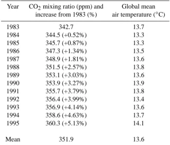
Table 2. CO2atmospheric levels and temperature conditions for the
1983–1995 interannual variability simulation.
Year CO2mixing ratio (ppm) and Global mean
increase from 1983 (%) air temperature (◦C)
1983 342.7 13.7 1984 344.5 (+0.52%) 13.3 1985 345.7 (+0.87%) 13.3 1986 347.3 (+1.34%) 13.5 1987 348.9 (+1.81%) 13.6 1988 351.5 (+2.57%) 13.8 1989 353.1 (+3.03%) 13.6 1990 353.9 (+3.27%) 13.9 1991 355.7 (+3.79%) 13.8 1992 356.4 (+3.99%) 13.4 1993 356.9 (+4.14%) 13.6 1994 358.6 (+4.63%) 13.7 1995 360.3 (+5.13%) 14.1 Mean 351.9 13.6
(1999) and for anthropogenic grasses by Goldewijk (2001) (De Noblet-Ducoudr´e and Peterschmitt, unpublished work). Initial conditions are taken from a 10-year equilibrated simu-lation based on 1983 climate and CO2conditions. The
inter-annual simulation, run for the 1983–1995 period, considers not only climate change but also annually varying CO2
atmo-spheric levels (Table 2): the CO2mixing ratio increases from
342.7 ppmv in 1983 up to 360.3 ppmv in 1995, a 5% increase over the 1983–1995 period (Keeling and Whorf 2005). The global and annual mean air temperature ranges from 13.3◦C to 14.1◦C (Table 2). The impact of key parameters, such as radiation extinction or temperature, on biogenic emissions is assessed running two sensitivity simulations, based on the 1983 climate and atmospheric CO2conditions.
In order to evaluate the impact of human activities on ecosystems distribution and hence on biogenic emissions, we perform a second set of simulations: tropical tion and European afforestation. For the tropical deforesta-tion simuladeforesta-tion, PFTs 2 and 3 (tropical broadleaf evergreen and raingreen trees), located in large regions of South Amer-ica, Africa and Indonesia, were replaced by 50% tropical crops and 50% tropical grasses (PFTs 11 and 13) while for the European afforestation simulation, we substituted crops (PFTs 12 and 13) with temperate broadleaf summer-green trees (PFT 6) in the regions between 37◦N–70◦N and
12◦W–44◦E. For these simulations, we have only addressed the issue of human induced land cover change and ignored the potential impacts of climate and CO2changes and of
nat-ural vegetation redistribution. We have then run one spe-cific year using only the 1983 climate and CO2conditions.
Although these simulations do not include dynamic vegeta-tion response to projected future climate and land use change,
they do represent predicted regional land use tendencies and their impact on regional and global biogenic emissions.
3 Global mean biogenic emissions for the 1983–1995 pe-riod
3.1 Comparison with other studies
Calculated global mean emissions for the 1983–1995 period are summarized and compared to previous estimates in Ta-ble 3. On a 13 years-mean basis, the global biogenic emis-sion source calculated by our model totals 752 TgC/yr of which 460 TgC/yr are isoprene, 117 TgC/yr monoterpenes, 106 TgC/yr methanol, 42 TgC/yr acetone, 15 TgC/yr ac-etaldehyde, 10 TgC/yr formaldehyde, 1.5 TgC/yr formic acid and 0.3 TgC/yr acetic acid. Our results are within the range found in the literature. The slight underestimation when compared with Guenther et al. (1995) estimate of 506 TgC/yr for isoprene global emission results from our accounting of the leaf age influence. In a sensitivity study, we have indeed neglected this parameter and found a global isoprene emis-sion of 506 TgC/yr, identical to Guenther et al. (1995) and closer to the values reported by Wang and Shallcross (2000) and Levis et al. (2003). Monoterpenes emission calculated by ORCHIDEE is close to the 127 TgC/yr given by Guenther et al. (1995). Monoterpenes and other VOC emissions may also be dependent on the leaf age, although, to the best of our knowledge, this effect has only been studied for isoprene and methanol emissions. Global emissions calculated for alde-hydes and acids are within the range given by Wiedinmyer et al. (2004). Biogenic emissions of acids total 1.8 TgC/yr from which formic acid emissions contribute to 1.5 TgC/yr, 3 times less than the production of organics by ozonolysis reaction, estimated to 5 TgC/yr (Baboukas et al., 2000).
Our estimate of global isoprene emission is similar to the 454 TgC/yr reported by Naik et al. (2004). Naik et al. (2004) considered a potential vegetation map with no agricultural land, which should lead to higher emissions than ours. How-ever, they assumed that grasses are not a major emitter of iso-prene (emission factor of 0) while we use emissions factors of 16 and 24 µgC/gdm/h for C3and C4grasses, respectively
(Guenther et al., 1995), that results in an additional emission of 90 TgC/yr into the atmosphere.
Sanderson et al. (2003) calculated global emissions of 484 TgC/yr for isoprene, a little higher than our results, which can be explained again by the difference in emission factors. Based on a sensitivity analysis, we found that adopt-ing the emission factors proposed by Sanderson et al. (2003) would lead to a global isoprene source about 485 TgC/yr.
Tao and Jain (2005) estimated isoprene global biogenic emissions to 601 TgC/yr, taking into account the leaf age influence. The emission factors were not assigned on a biome basis but depended on the grid cell considered and
Table 3. Global mean biogenic emissions (TgC/yr) and contribution to total biogenic VOCs (%) over the period 1983–1995.
TgC/yr Isoprene Monoterpenes Methanol Acetone Acetaldehyde Formaldehyde Formic acid Acetic acid TOTAL This study 460 117 106 42 15 10 1.5 0.3 752
(61%) (15%) (14%) (6%) (2%) (1.5%) (0.2%) (0.05%)
Galbally and Kirstine (2002)
37.5
Guenther et al. (1995) 503 127 1150
Horowitz et al. (2003) 107
Levis et al. (2003) 507 33 692
Naik et al. (2004) (poten-tial vegetation)
454 72 Sanderson et al. (2003) 484
Tie et al. (2003) 108 Wang and Shallcross
(2000)
530
Wiedinmyer et al. (2004) 50–250 10–50 10–50 2–10 0.4–2 0.4–2
thus showed a strong variability throughout the world, which is not the case in our study.
If the results calculated with our model compare well with other estimates on a global basis, they do emphasize the sen-sitivity of computed biogenic emissions to the chosen emis-sion factors. Indeed, an emisemis-sion factor allocation based only on PFTs may not be sufficient to take into account the large emission factor variability from one ecosystem to another and to provide a realistic regional distribution of biogenic compounds, which can be of great importance, especially for atmospheric chemistry studies. Serc¸a et al. (2001) investi-gated isoprene emission in a forest-site of the Republic of Congo, as part of the EXPRESSO program, and found that of the 28 species from the mixed forest, only 3 were high iso-prene emitters (emission rate over 16 µgC/g/h) while in the monospecific forest, 2 species had high emission rates (45 and 62 µgC/g/h), for the same conditions of temperature and PAR. Growth environmental conditions such as long-term variation in light, temperature and water stress presumably regulate emissions capacity as observed for isoprene (Harley et al., 1999; Hanson and Sharkey, 2001a; P´etron et al., 2001) and monoterpenes (Staudt et al., 2003). VOC biogenic emis-sions calculation should then integrate those parameters and a more complex emission factors prescription, depending not only on PFT but also on the geographical location should then be used, as proposed by Guenther et al. (2006) in the MEGAN model.
Galbally and Kirstine (2002) estimated methanol emis-sions by flowering plants to 100 Tg of methanol per year (37.5 TgC/yr), based on plant structure and metabolic prop-erties. This work, which leads to significantly lower emis-sions compared to ours, uses a completely different approach based on a plant physiology model. Horowitz et al. (2003) estimated biogenic methanol emissions of 108 TgC/yr, based on the emission ratio to isoprene found by Guenther et al. (2000) for North America. Tie et al. (2003) studied the impact of biogenic methanol on tropospheric oxidants
as-0 1 2 3 4 5 5:00 7:00 9:00 11:00 13:00 15:00 17:00 19:00 21:00 Is o p re n e ( u g /m ²/s )
Fig. 3. Comparison of the ORCHIDEE results with
measure-ments of the ECHO campaign (Spirig et al., 2005) for isoprene
(µg/m2/s). Monthly mean ORCHIDEE isoprene emissions for July
(red squares) and variance (red bars) are compared to the mean di-urnal cycle (black squares) measured during the ECHO campaign, and to the fluxes reported day-by-day (black crosses).
suming a global surface methanol source of 117 TgC/yr, of which 92% is due to biogenic sources, that is 108 TgC/yr, which is very similar to our results.
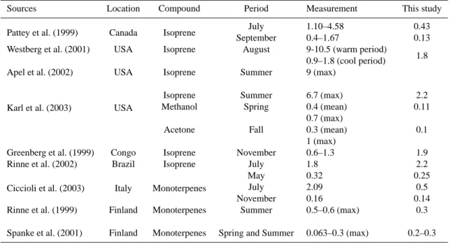
Comparison of the ORCHIDEE monthly mean emissions fluxes over the 1983–1995 with a limited compilation of measurements is given in Table 4 and show that the results of our model are broadly within the range of selected mea-surements. In the Fig. 3, the diurnal isoprene emissions cy-cle calculated by our model is compared to measurements of the ECHO campaign (Spirig et al., 2005), which took place in North-West Germany in July 2003, and we can see that in this case, the diurnal variation of isoprene fluxes is quite well captured by our model. It is of course difficult to evaluate a global model based only on a few comparisons with measure-ments, and a more detailed validation is required. Neverthe-less, the examples shown in Table 4 and Fig. 3 underline that our model is generally consistent with the measurements.
Fig. 4. Global mean biogenic emissions over the 1983–1995 period in kgC/m2/s in January (left column) and July (right column) for isoprene, monoterpenes, methanol and ORVOC.
Table 4. Comparison of the ORCHIDEE 1983-1995 mean biogenic emissions with on-site measurements (mgC/m2/h).
Sources Location Compound Period Measurement This study
Pattey et al. (1999) Canada Isoprene July 1.10–4.58 0.43
September 0.4–1.67 0.13
Westberg et al. (2001) USA Isoprene August 9-10.5 (warm period)
0.9–1.8 (cool period) 1.8
Apel et al. (2002) USA Isoprene Summer 9 (max)
Karl et al. (2003) USA
Isoprene Summer 6.7 (max) 2.2
Methanol Spring 0.4 (mean)
0.7 (max)
0.11
Acetone Fall 0.3 (mean)
1 (max)
0.1
Greenberg et al. (1999) Congo Isoprene November 0.6–1.3 1.9
Rinne et al. (2002) Brazil Isoprene July 1.8 2.2
Ciccioli et al. (2003) Italy Monoterpenes
May 0.32 0.25
July 2.09 0.5
November 0.16 0.14
Rinne et al. (1999) Finland Monoterpenes Summer 0.5–0.6 (max) 0.3
Spanke et al. (2001) Finland Monoterpenes Spring and Summer 0.063–0.3 (max) 0.2–0.3
3.2 Attribution of global emissions to PFTs and VOC com-ponents
Three major biogenic compounds are emitted: isoprene, which contribute to more than 61% to the global annual bio-genic emissions, monoterpenes (15%) and methanol (14%) (Table 3). However, even if other compounds such as ace-tone (6%), acetaldehyde or formaldehyde (2% and 1.5%), formic (0.2%) and acetic (0.05%) acids are emitted in smaller individual quantities, these other species total a significant amount of reactive compounds emitted to the atmosphere, of almost 70 TgC/yr.
Figure 4 shows the geographical distribution of calculated emissions for isoprene, monoterpenes, methanol and OR-VOC (defined as other reactive OR-VOCs with lifetime smaller than 1 day, and calculated with a constant emission factor of 1.5 µgC/gdm/h for every PFTs, Guenther et al., 1995). In January, significant emissions of 2–8×10⁻¹⁰kgC/m2/s for isoprene and 5–20×10−11kgC/m2/s for monoterpenes are calculated in the southern hemisphere and tropical regions. Isoprene is primarily emitted in tropical regions, because tropical vegetation (PFTs 2 and 3) are characterized by both high leaf area index up to 7–8 m2/m2 (Fig. 2) and strong emissions factors (Table 1). High isoprene emissions occur all year in these regions. In July, high isoprene emissions by 3–10×10−10kgC/m2/s are also calculated locally in the east coast of the US and in southern Spain due to a high density of temperate broadleaf summergreen trees (PFT 6). Monoterpenes emission levels are also significant in tropical regions, but do not extend as much as isoprene emissions to
the south of the Amazon region. In July, high monoterpenes emissions of 10–20×10−11kgC/m2/s are found in Siberia and Canada, whereas tropical regions contribute much less to the global monoterpenes emission. The biogenic emissions of other VOCs such as acetone, acids and aldehydes have the same pattern because their emissions factors and emis-sion parameterization are similar to monoterpenes. Methanol emissions are particularly high in tropical regions such as In-dia or the southern Asia, due to a high density of crops, a strong methanol emitter, in those regions. In July, methanol emissions range from 6 to over 20×10−11kgC/m2/s in In-donesia.
Table 5 shows the contribution of various PFTs and re-gions to the global biogenic emissions on a 1983–1995 mean basis. The contribution of tropical vegetation (PFTs 2 and 3) to the global emissions are 61% for isoprene, 53% for monoterpenes but only 32% for methanol. Crops (PFTs 12 and 13) are significant methanol emitters, contributing to 44% of global methanol emissions, but are much less im-portant for isoprene and other VOCs (6–6.5% of global emissions). Tropical regions are a major contributor to global annual biogenic emissions: 83% of isoprene, 69% of monoterpenes and 66% of methanol global annual emissions originate from tropical regions (30◦S–30◦N). In our study, grasses (PFTs 10 and 11) are a significant source of isoprene contributing to 20% of the global yearly emission. This result is in contrast with other studies (Levis et al., 2003; Naik et al., 2004), which assume that grasses do not emit isoprene at a significant level. Even if the maximum leaf area index for grasses is only 2.5 m2/m2, we consider quite high isoprene
Table 5. Contribution of PFTs and various regions to global biogenic emissions in TgC/yr (and %) on a 1983–1995 mean basis. Tropical
regions are defined between +/−30◦and 0◦, higher latitude regions are defined between +/−30◦and +/−90◦.
PFT Isoprene Monoterpenes Methanol Acetone
Tropical broadleaf evergreen tree 258 (56%) 58 (50%) 31 (30%) 21 (50%)
Tropical broadleaf raingreen tree 23 (5%) 3.5 (3%) 2 (2%) 1.5 (3%)
Temperate needleleaf evergreen tree 7 (2%) 13 (11%) 7 (7%) 5 (11%)
Temperate broadleaf evergreen tree 12 (3%) 4.5 (4%) 2.5 (2%) 2 (4%)
Temperate broadleaf summergreen tree 32 (7%) 3 (2%) 1.5 (1%) 1 (2%)
Boreal needleleaf evergreen tree 5 (1%) 11 (9%) 6 (5%) 4 (9%)
Boreal broadleaf summergreen tree 1.5 (0.33%) 2 (2%) 1 (1%) 0.8 (2%)
Boreal needleleaf summergreen tree 1 (0.2%) 1 (0.9%) 1 (0.6%) 0.4 (0.9%)
C3 Grass 44 (10%) 8 (7%) 4.5 (4%) 3 (7%) C4 Grass 46 (10%) 7 (6%) 4 (4%) 3 (6%) C3 Agriculture 15 (3%) 3 (3%) 22 (22%) 1 (3%) C4 Agriculture 16 (3.5%) 3 (3%) 23 (22%) 1 (3%) Tropics 381 (83%) 82 (69%) 70 (66%) 30 (70%) Tropical South 213 (46%) 45 (38%) 33 (31%) 16 (38%) Tropical North 168 (37%) 37 (31%) 37 (35%) 13.5 (31%) Higher South 8 (2%) 2 (2%) 3 (2%) 0.8 (2%) Higher North 71 (15%) 34 (29%) 33 (31%) 12 (29%) Europe 14 (3%) 5 (4%) 7 (6%) 2 (4%) Global 460 117 106 42
emission factors, as given in Guenther et al. (1995) for hot and cool grass/shrub, and the spatial coverage and density of grasses is often very high. It is thus a critical point to know if grasses can be considered as an isoprene emitter or not since a very different regional isoprene emissions dis-tribution would arise. Several studies emphasized the low isoprene emission level of grasses but the number of species of grass that emit isoprene is highly uncertain (Holzinger et al., 2002; Wiedinmyer et al., 2004). Moreover, high isoprene emission capacities have been measured for shrubs (Guen-ther et al., 1999b), which are included in PFTs 10 and 11. Grasses are of less importance for other VOCs emissions, for which their contribution is between 8 and 13%.
3.3 Sensitivity tests to parameters choices
Additional simulations were conducted for the year 1983 to assess the sensitivity of biogenic emissions to key parameters such as temperature, leaf age or radiation extinction within the canopy (Eq. 1). We estimated that the radiation extinc-tion considered for isoprene emissions leads to the halving of isoprene emission, decreasing from 983 TgC/yr without radiation extinction to 478 TgC/yr. Accounting for the leaf age influence leads to a decrease in global emissions of 10% for isoprene and 27% for methanol. Increasing the surface temperature (used as a surrogate of leaf temperature) in the biogenic emissions model globally by 1◦C leads to an in-crease in the global emission of 11% for isoprene and 9% for
other compounds (478 TgC/yr to 529 TgC/yr for isoprene, 119 TgC/yr to 129 TgC/yr for monoterpenes, 106 TgC/yr to 116 TgC/yr for methanol and 43 TgC/yr to 47 TgC/yr for ace-tone) resulting in a substantial additional total emission of VOCs to the atmosphere of 78 TgC/yr. Considering the dif-ficulty in estimating leaf temperature and the canopy en-ergy balance highlights the large uncertainty in calculated biogenic emissions. The next step for biogenic emission model improvement would be to calculate the leaf temper-ature for sunlit and shaded leaves, as suggested by measure-ments given by Harley et al. (1997).
4 Interannual variability of biogenic emissions over the period 1983–1995
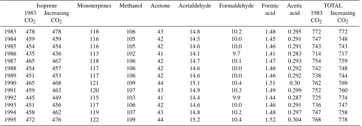
In this section, the impact of the variability in climate con-ditions and of increasing atmospheric CO2 concentrations
on biogenic emissions is investigated over the period 1983– 1995. As shown in Table 6, the total global emission of all biogenic compounds ranges from 717 TgC/yr in 1986 to 778 TgC/yr in 1995, that is a 8.5% increase between both extreme values, and has a variability of +/−16 TgC/yr over the 1983–1995 period. In order to asses the impact of atmo-spheric CO2mixing ratio increase on biogenic emissions, we
performed a second 1983–1995 simulation considering the 1983 CO2atmospheric level (342.7 ppmv) for the whole
Table 6. Interannual variability of biogenic emissions over the 1983-1995 period (TgC/yr).
Isoprene Monoterpenes Methanol Acetone Acetaldehyde Formaldehyde Formic Acetic TOTAL 1983 Increasing acid acid 1983 Increasing
CO2 CO2 CO2 CO2 1983 478 478 118 106 43 14.8 10.2 1.48 0.295 772 772 1984 459 459 116 105 42 14.5 10.0 1.45 0.291 747 748 1985 454 454 116 105 42 14.6 10.0 1.46 0.291 743 743 1986 435 436 113 102 41 14.1 9.7 1.41 0.283 714 717 1987 465 467 118 106 42 14.7 10.1 1.47 0.293 754 759 1988 454 457 117 106 42 14.6 10.0 1.46 0.292 742 748 1989 451 453 117 106 42 14.6 10.0 1.46 0.292 738 744 1990 465 468 121 109 44 15.1 10.4 1.51 0.30 762 769 1991 459 463 120 107 43 14.9 10.3 1.49 0.299 752 760 1992 445 449 115 103 41 14.4 9.9 1.44 0.287 725 734 1993 451 456 117 106 42 14.6 10.0 1.46 0.291 736 747 1994 458 462 119 107 43 14.8 10.2 1.48 0.297 747 758 1995 472 476 122 109 44 15.2 10.4 1.52 0.304 768 778
“constant CO2” simulation and the “increasing CO2”
simu-lation reaches 4 TgC/yr for isoprene and 10 TgC/yr for the total VOC, which corresponds to 0.8% and 1.3% difference, respectively, linked to an increase in foliar biomass under in-creasing atmospheric CO2conditions.
An important control on climate conditions in tropical re-gions is the occurrence of El Ni˜no and La Ni˜na events, which lead to major warming and cooling cycles in the eastern and central Pacific. The Southern Oscillation Index (SOI), de-fined as the pressure difference between Tahiti and Darwin, provides the intensity of El Ni˜no and La Ni˜na episodes. As shown in Table 6, biogenic emissions are generally higher during El Ni˜no years (1983, 1987, 1990–1991 and 1994– 1995), and lower during La Ni˜na years (1984–1985, 1988– 1989). A similar finding was obtained by Naik et al. (2004) over the period 1971–1990. However there is an exception for the 1992–1993 weak El Ni˜no event for which global bio-genic emissions are lower than average. For those two years, the El Ni˜no effect on the temperature increase in the western part of South America is very small (with a maximum in-crease of 0.4◦C in northern part of South America compared to 1983–1995 mean temperature of 26–28◦C in this region), and does not impact significantly on biogenic emissions lev-els, whereas a temperature decrease can be noted southward of Brazil and in Central Africa, leading to a decrease in biogenic emissions. The comparison between the SOI and the calculated monthly global isoprene emissions anomalies (Fig. 5) indicates a negative correlation. The correlation co-efficient (r) between the SOI and monthly global biogenic emissions anomalies, calculated for the period 1983–1995, is −0.28 for isoprene, −0.14 for monoterpenes and −0.01 for methanol. These values are in qualitative agreement with Naik et al. (2004) but of smaller absolute correlation (−0.54 for isoprene and −0.24 for monoterpenes for 1971–1990, in Naik et al., 2004). The correlation coefficients obtained
Comparison between the SOI and biogenic emissions anomaly
-40 -30 -20 -10 0 10 20 30 1983 1985 1987 1989 1991 1993 1995 SO I -6 -4 -2 0 2 4 6 Is opr e n e
Fig. 5. Comparison between the Southern Oscillation Index SOI (black line) and the simulated anomalies of global monthly biogenic isoprene emissions (grey line, TgC/month) for the 1983–1995 pe-riod.
Fig. 6. Square correlation coefficient (r2) between the Southern Oscillation Index and biogenic isoprene emissions for the 1983– 1995 period.
are rather small but it is however interesting to note that the correlation between biogenic emissions and SOI is some-what higher in tropical regions compared to other regions, as shown in Fig. 6 for isoprene.
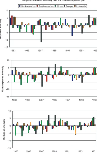
As indicated by Fig. 6, the variability in biogenic emis-sions over the 13 years of the simulation varies from one
Biogenic emission anomaly over the 1983-1995 period (%) -15 -10 -5 0 5 10 1983 1985 1987 1989 1991 1993 1995 Is o p re ne a n o m a ly
North America South America Africa Europe Indonesia
-15 -10 -5 0 5 10 1983 1985 1987 1989 1991 1993 1995 Mo n o te rp en es an o m aly -15 -10 -5 0 5 10 1983 1985 1987 1989 1991 1993 1995 M e th an o l an o m al y
Fig. 7. Variability of annual biogenic emissions anomaly based on 1983–1995 mean emissions calculated for North America, South America, Africa, Europe and Indonesia for isoprene (upper panel) , monoterpenes (middle panel) and methanol (lower panel).
region to another. To further illustrate this feature, Fig. 7 shows the annual emission anomaly in %, compared to 1983– 1995 mean emissions, calculated for isoprene, monoterpenes and methanol for 5 regions: North America (150 W–52 W, 12 N–70 N), South America (85 W–34 W, 60 S–15 N), Africa (18 W–51 E, 35 S–37 N), Europe (10 W–50 E, 35 N–72 N) and Indonesia (60 E–160 E, 11 S–40 N). Biogenic emissions variability is strongly affected by the evolution of environ-mental conditions such as radiation, temperature or leaf area index. In Europe, in relation to a strong air temperature vari-ability over the period 1983–1995, the emission anomaly has the largest variability from −11.5% to +6.8% for isoprene, from −8.1% to +7.2% for monoterpenes and from −5.6% to +7.2% for methanol. In 1987, biogenic emissions have a strong negative anomaly in Europe, where annual mean air temperature differs the most from 1983–1995 mean tem-perature compared to other regions studied, especially for
Fig. 8. PFTs distribution considered for the Tropical deforestation (upper panel) and European afforestation (lower panel) scenarios.
isoprene (−11.5%) and monoterpenes (−8.1%). The am-plitude of the isoprene emission anomaly is about 10% for North and South America and Africa, but smaller for Indone-sia (7.5%). Variation in the emission anomaly is lowest in Indonesia (−3.3% to +3%) and North America (−4.2% to +3.1%) for monoterpenes and in North (−2.9% to 2.8%) and South (−3.9% to +3.3%) America for methanol.
5 Impacts of tropical deforestation and European af-forestation on global biogenic emissions
5.1 Tropical deforestation
Figure 9 illustrates the change in total annual mean leaf area index between the tropical deforestation scenario and the 1983 control run (1983 simulation with non-modified present vegetation map). In the tropical regions with low
Table 7. Global biogenic emissions (TgC/yr) and changes (%) for the tropical deforestation simulation and European afforestation simulation compared to the control run (nc: no change).
TgC/yr (%) 1983 Control Run Tropical deforestation European afforestation
Global Tropics Europe Global Tropics Global Europe
Isoprene 478 396 15 339 (−29%) 257 (−35%) 497 (+4%) 33 (+126%) Monoterpenes 118 81 5 84 (−29%) 48 (−41%) 118 (−0.1%) 6 (+13%) Methanol 106 70 7 130 (+22%) 93 (+33%) 102 (−3.5%) 3 (−51%) Acetone 43 29 2 30 (−29%) 17 (−42%) 43 (−0.2%) 2 (+10%) Acetaldehyde 15 10 0.64 10 (−29%) 6 (−42%) 15 (nc) 0.7 (+16%) Formaldehyde 10 7 0.44 7 (−30%) 4 (−44%) 10 (nc) 0.5 (+14%) Formic acid 1.5 1 0.06 1 (−29%) 0.6 (−44%) 1.48 (nc) 0.07 (+14%) Acetic acid 0.29 0.20 0.013 0.21 (−27%) 0.12 (−40%) 0.29 (nc) 0.015 (+15%) TOTAL 772 595 30 602 (−22%) 426 (−20%) 787 (+2%) 46 (+54%)
precipitation, such as the southern part of Brazil, the LAI is quite small in the control run (1–3 m2/m2). Deforesta-tion leads to a small increase in LAI in this region between 1 and 1.5 m2/m2. In significant parts of Amazonia, Central Africa and Indonesia, a large decrease in LAI in the range 2–4.5 m2/m2is modelled.
Tropical deforestation has a major impact on biogenic emissions, as shown in Table 7. On a global basis, methanol emissions increase by 22%, in relation to crops coverage expansion, whereas isoprene and other VOC emissions de-crease by 27–30%. If we consider tropical regions only, a 33% increase in methanol emissions occurs and a 35–44% decrease is predicted for isoprene and other VOCs. The isoprene emission decrease calculated for East Asia reaches 26%, which is closed to the 30% decrease calculated by Steiner et al. (2002). Moreover, as illustrated in Fig. 9 by the zonal mean difference of biogenic emissions between the tropical deforestation simulation and the control run, the sea-sonality of emissions is also affected by the tropical defor-estation. The decrease in isoprene zonal mean emissions, governed by a reduction in both LAI and emission factors under tropical deforestation conditions, is significant all year long (−0.5×10⁻¹⁰ to −2×10⁻¹⁰kgC/m2/s) and peaks in March north of the Equator and in September south of the Equator (−2×10⁻¹⁰ to −3.5×10⁻¹⁰kgC/m2/s). Methanol zonal mean emissions increase by 0.5–4×10⁻¹¹kgC/m2/s throughout the year, and by 4–5×10⁻¹¹kgC/m2/s from Jan-uary to September between 0◦and 10◦S. A decrease in zonal
mean methanol emissions is also modelled north of the equa-tor in March, and south of the equaequa-tor in September (−0.5 to
−2.5×10⁻¹¹kgC/m2/s). This reduction in methanol emis-sions is due to the large decrease in LAI in these regions, and occurs despite the significantly larger methanol emission factors of crops compared to tropical trees (Table 1). These results illustrate the importance of tropical regions as a major and very sensitive biogenic emissions source, under pressure from rapid and strong land use change.
5.2 European afforestation
Under the European afforestation scenario, the total annual mean LAI tends to decrease by 1 m2/m2 over large regions of Europe, and up to 2 m2/m2 in Great-Britain, where the highest LAI decrease occurs. LAI increases locally by up to 2.5 m2/m2 in the centre of Europe, northward of the Black Sea (Fig. 10). This result, which can seem surprising, is linked to the fact that we turn perennial crops into a sum-mergreen vegetation, both characterized by a maximum LAI of 5 m2/m2. We know that perennial crops are not realis-tic and this is being changed in ORCHIDEE (Gervois et al., 2004). Nevertheless, this bias in the representation of crops only marginally affects the results discussed here.
Globally, emissions are not significantly affected by Eu-ropean afforestation: a 4% increase is calculated for iso-prene and a 3.5% decrease for methanol, and less than 0.2% for other VOCs is computed. However, at the European scale, the impact is very significant, with a 51% decrease in methanol emissions, an increase of 126% for isoprene and 10–15% for other VOCs, leading to an increase in total bio-genic emissions in Europe of 54%. The very large increase in the isoprene emission factor (multiplied by 9 compared to crops) leads to a large overall increase in biogenic emissions, despite the small decrease in LAI. The combined effect of total LAI and emission factor reduction leads to a large de-crease in methanol emissions, lasting through the year since methanol crops emissions also occur in winter in the control run while there is no emission by PFT 6 (summergreen trees) during winter. The change in zonal mean emissions, given in Fig. 10, shows a 0.5×10⁻¹⁰to 4.5×10⁻¹⁰kgC/m2/s increase in zonal mean isoprene emissions from April to November. Zonal mean methanol emissions decrease by 0.5×10⁻¹¹– 1.5×10⁻¹¹kgC/m2/s, between January and March and af-ter October, and by 1.5×10⁻¹¹–5×10⁻¹¹kgC/m2/s, during spring and summer. For both isoprene and methanol, the maximum change in zonal mean emissions occurs in July
Fig. 9. Impact of a tropical deforestation scenario on total annual
mean LAI (m2/m2) (upper panel), zonal mean isoprene (middle
panel) and methanol (lower panel) emissions compared to the 1983 control run.
between 42◦N and 52◦N. Even though global biogenic emis-sions are not significantly affected by European afforesta-tion, its impact on regional emissions is very large and could strongly influence tropospheric chemistry mechanisms both within and outside Europe.
The vegetation distribution change considered in our study is only intended to be a sensitivity experiment and probably overestimates the future changes. Nevertheless, the results obtained in the tropical deforestation and European reforesta-tion simulareforesta-tions underline the strong impact of vegetareforesta-tion distribution alteration on VOC biogenic emissions as well as the high dependency of emission levels to the evolution of land management.
Fig. 10. Impact of a European afforestation scenario on total
an-nual mean LAI (m2/m2)(upper panel), zonal mean isoprene
(mid-dle panel) and methanol (lower panel) emissions compared to the 1983 control run.
6 Conclusion
A biogenic emission scheme has been integrated in the global vegetation model ORCHIDEE in order to calculate biogenic emissions of isoprene, monoterpenes, methanol, acetone, ac-etaldehyde, formaldehyde, as well as formic and acetic acids at the global scale. In order to study the impact of climate and land use changes on biogenic emissions, several simula-tions are performed. Global mean emissions of 460 TgC/yr for isoprene, 117 TgC/yr for monoterpenes, 106 TgC/yr for methanol and 42 TgC/yr for acetone are calculated over the
period 1983–1995. Tropical regions are identified as the pri-mary source of global biogenic VOCs, contributing to 83% of isoprene, 69% of monoterpenes and 66% of methanol global annual emissions. The interannual simulation predicts a substantial variability in biogenic emissions over the 1983– 1995 period. The total global and annual emissions of the summed VOCs range from 718 TgC/yr (1986) to 778 TgC/yr (1995), i.e. an 8.4% variability over 1983–1995. The vari-ability in emissions is markedly different from one region to another. Among the regions studied, biogenic emissions vari-ation compared to 1983–1995 mean emissions was found to be the highest in Europe and the smallest in Indonesia (iso-prene and monoterpenes) and North America (methanol).
Two scenarios of land use change, tropical deforestation and European afforestation, have been considered to exam-ine the sensitivity of biogenic emissions to the vegetation distribution alteration. On the global scale, our calculations indicate that the tropical deforestation leads to a methanol emission increase by 22%, whereas isoprene and other VOCs emissions decrease by 27–30%. If we consider tropical re-gions only, a 33% increase is calculated for methanol emis-sions, and a 35–44% decrease is estimated for isoprene and other VOCs. Global emissions are not significantly affected by the European afforestation, but at the european scale, the impact is much more important, with a 51% decrease for methanol emissions and an increase of 126% for isoprene and 10–15% for other VOCs, leading to an increase in the total biogenic emissions in Europe of 54%.
Our results are generally consistent with previous studies. It should be noted that our study also takes into account fea-tures such as the leaf age for isoprene and methanol emis-sions. Based on a sensitivity test, we estimated that account-ing for the leaf age influence leads to a decrease in global emissions of 10% for isoprene and 27% for methanol. Fu-ture biogenic emission studies need to consider if grasses can be considered as a significant isoprene emitter or not as this could greatly affect regional isoprene emissions distribution. Indeed, we calculate that grasses contribute to nearly 20% of the isoprene global and annual emission whereas recent stud-ies such as Levis et al. (2003) and Naik et al. (2004) assume that the grass isoprene emission factor is negligible. De-pending on this choice, our emission estimates for land-use change scenarios, such as European afforestation and Tropi-cal deforestation, could be significantly different.
Air temperature above the canopy is used to calculate bio-genic emissions when a more accurate canopy energy bal-ance, estimating leaf temperature is not available. Pier and McDuffie (1997) observed, comparing measurements and model emissions, that calculating biogenic emissions based on air temperature leads to a slight underestimation of high emission rates. Hanson and Sharkey (2001b) pointed out that biogenic emission models should be adjusted to account for variation in response to temperature and light levels during vegetation growth, which could be done simply by altering the emission capacity (other coefficients used in light and
temperature emissions dependencies were not found to be sensitive to environmental growth conditions). Increasing globally the leaf temperature used in the biogenic emissions model by 1◦C leads to an increase in the global emission of 11% for isoprene and 9% for other compounds (478 TgC/yr to 529 TgC/yr for isoprene, 119 TgC/yr to 129 TgC/yr for monoterpenes, 106 TgC/yr to 116 TgC/yr for methanol and 43 TgC/yr to 47 TgC/yr for acetone) resulting in a substantial additional emission of VOCs to the atmosphere of 78 TgC/yr. The difficulty to estimate the leaf temperature and the canopy energy balance appears as a major uncertainty in calculating biogenic emissions. A next step for biogenic emissions mod-els improvement would be to calculate the leaf temperature for sunlit and shaded leaves, as suggested by the measure-ments of Harley et al. (1997).
The distribution, as well as the diversity, of vegetation throughout the world is under pressure from both direct anthropogenic changes, such as deforestation and agricul-ture expansion, driven by population growth, and indirect changes, also affected partly by human activities, includ-ing atmospheric CO2 and climate evolution. Alcamo et
al. (1996) suggested that in the next 50 years, land-cover conversion may occur predominantly in the tropical and sub-tropical regions, in response to projections of demographic growth and economic activity. The consequences of such changes not only on biogenic emissions but also on the tro-pospheric gas phase and particulate chemistry could be sig-nificant. The use of dynamic global vegetation models, for future scenarios, and more generally for climate and land use change studies, is an essential next step. Neverthe-less, important points, such as the pattern and dependency of emissions on environmental conditions for compounds other than isoprene and monoterpenes, and the response of foliar density and biogenic emission factors to CO2and
cli-mate change, are still under debate. Rosenstiel et al. (2003) showed that under increased atmospheric CO2 level from
430 ppmv to 800 and 1200 ppmv, the isoprene production was reduced by 21% and 41% while above-ground biomass accumulation was enhanced by 60% and 82%. We can rea-sonably consider that considering this influence in our study would not change significantly the estimates calculated over the 1983–1995 period, characterized by a 5% increase of the atmospheric CO2 but could however be subsequent on
longer time-scales. The influences of those various parame-ters could affect emissions levels significantly, and more in-formation is needed to reduce the estimates uncertainty and improve our understanding of biosphere-atmosphere interac-tions.
Acknowledgements. We thank J.-Y. Peterschmitt for his help in the
preparation of the global vegetation maps. Useful comments and discussions on this work by P. Friedlingstein, D. Serc¸a, G. Krin-ner, A. Guenther and S. Gervois are gratefully acknowledged. Computer time has been provided by the C.C.R.T under project
p24. This work was partly funded by the European projects
(GOCE-CT-2003-505539). G. Folberth acknowledges support provided by the Canadian Centre for Climate Modelling and Analysis, Meteorological Service of Canada.
Edited by: U. Lohmann
References
Alcamo, J., Kreileman, G. J. J., Bollen, J. C., vandenBorn, G. J., Gerlagh, R., Krol, M. S., Toet, A. M. C., and deVries, H. J. M.: Baseline scenarios of global environmental change, Global En-vironmental Change-Human and Policy Dimensions, 6(4), 261– 303, 1996.
Andreae, M. O. and Crutzen, P. J.: Atmospheric aerosols: bio-geochemical sources and role in atmospheric chemistry, Science, 276, 1052–1058, 1997.
Apel, E. C., Riemer, D. D., Hills, A., Baugh, W., Orlando, J., Faloona, I., Tan, D., Brune, W., Lamb, B., Westberg, H., Carroll, M. A., Thornberry, T., and Geron, C. D.: Mea-surement and interpretation of isoprene fluxes and isoprene, methacrolein, and methyl vinyl ketone mixing ratios at the PROPHET site during the 1998 Intensive, J. Geophys. Res., 107, D3, doi:10.1029/2000JD000225, 2002.
Baboukas, E. D., Kanakidou, M., and Mihalopoulos, N.: Car-boxylic acids in gas and particulate phase above the Atlantic Ocean, J. Geophys. Res.-Atmos., 105(D11), 14 459–14 471, 2000.
Barket, D. J., Grossenbacher, J. W., Hurst, J. M., Shepson, P. B., Olszyna, K., Thornberry, T., Carroll, M. A., Roberts, J., Stroud, C., Bottenheim, J., and Biesenthal, T.: A study of the NOx de-pendence of isoprene oxidation, J. Geophys. Res., 109, D11, doi:10.1029/2003JD003965, 2004.
Ciais, P., Reichstein, M., Viovy, N., Granier, A., Ogee, J., Allard, V., Aubinet, M., Buchmann, N., Bernhofer, C., Carrara, A., Cheval-lier, F., De Noblet, N., Friend, A. D., Friedlingstein, P., Grun-wald, T., Heinesch, B., Keronen, P., Knohl, A., Krinner, G., Loustau, D., Manca, G., Matteucci, G., Miglietta, F., Ourcival, J. M., Papale, D., Pilegaard, K., Rambal, S., Seufert, G., Sous-sana, J. F., Sanz, M. J., Schulze, E. D., Vesala, T., and Valentini, R.: Europe-wide reduction in primary productivity caused by the heat and drought in 2003, Nature, 437(7058), 529–533, 2005. Ciccioli, P., Brancaleoni, E., Frattoni, M., Marta, S., Brachetti, A.,
Vitullo, M., Tirone, G., and Valentini, R.: Relaxed eddy accu-mulation, a new technique for measuring emission and deposi-tion fluxes of volatile organic compounds by capillary gas chro-matography and mass spectrometry, J. Chromatogr. A, 985(1–2), 283–296, 2003.
Claeys, M., Graham, B., Vas, G., Wang, W., Vermeylen, R., Pashyn-ska, V., Cafmeyer, J., Guyon, P., Andreae, M. O., Artaxo, P., and Maenhaut, W.: Formation of secondary organic aerosols through photooxidation of isoprene, Science, 303(5661), 1173– 1176, 2004.
De Rosnay, P. and Polcher, J.: Modeling root water uptake in a complex land surface scheme coupled to a GCM, Hydrol. Earth Syst. Sci., 2, 239–256, 1998, mboxhttp://www.hydrol-earth-syst-sci.net/2/239/1998/.
Ducoudr´e, N., Laval, K., and Perrier, A.: SECHIBA, a new set of parameterizations of the hydrologic exchanges at the
land-atmosphere interface within the LMD atmospheric general cir-culation model, J. Climate, 6, 248–273, 1993.
Fehsenfeld, F., Calvert, J., Fall, R., Goldan, P., Guenther, A. B., Hewitt, C. N., Lamb, B., Liu, S., Trainer, M., Westberg, H., and Zimmerman, P.: Emissions of volatile organic compounds from vegetation and the implications for atmospheric chemistry, Global Biogeochem. Cycles, 6(4), 389–430, 1992.
Galbally, I. E. and Kirstine, W.: The production of methanol by flowering plants and the global cycle of methanol, J. Atmos. Chem., 43, 195–229, 2002.
Ganzeveld, L. and Lelieveld, J.: Impact of Amazonian defor-estation on atmospheric chemistry, Geophys. Res. Lett., 31, 6, doi:10.1029/2003GL019205, 2004.
Gervois, S., De Noblet-Ducoudr´e, N., Viovy, N., Ciais, P., Brisson, N., Seguin, B., and Perrier, A.: Including croplands in a global biosphere model: methodology and evaluation at specific sites, Earth Interactions, 8, Paper 16, 1–25, 2004.
Goldewijk, K. K.: Estimating global land use change over the past 300 years: The HYDE Database, Global Biogeochem. Cycles, 15(2), 417–433, 2001.
Greenberg, J. P., Guenther, A., Madronich, S., Baugh, W., Ginoux, P., Druilhet, A., Delmas, R., and Delon, C.: Biogenic volatile organic compound emissions in central Africa during the Ex-periment for the Regional Sources and Sinks of Oxidants (EX-PRESSO) biomass burning season, J. Geophys. Res., 104(D23), 30 659–30 671, 1999.
Griffin, R. J., Cocker, D. R., Seinfeld, J. H., and Dabdub, D.: Es-timate of global atmospheric organic aerosol from oxidation of biogenic hydrocarbons, Geophys. Res. Lett., 26(17), 2721–2724, 1999.
Guenther, A., Hewitt, C. N., Erickson, D., Fall, R., Geron, C., Graedel, T., Harley, P., Klinger, L., Lerdau, M., McKay, W. A., Pierce, T., Scholes, B., Steinbrecher, R., Tallamraju, R., Tay-lor, J., and Zimmerman, P.: A global model of natural volatile organic compound emissions, J. Geophys. Res., 100(D5), 8873– 8892, 1995.
Guenther, A., Baugh, B., Brasseur, G., Greenberg, J., Harley, P., Klinger, L., Serc¸a, D., and Vierling, L.: Isoprene emis-sion estimates and uncertainties for the Central African EX-PRESSO study domain, J. Geophys. Res., 104(D23), 30 625– 30 639, 1999a.
Guenther, A., Archer, S., Harley, P., Helmig, D., Klinger, L., Vier-ling, L., Wildermuth, M., Zimmerman, P., and Zitzer, S.: Bio-genic hydrocarbon emissions and landcover/climate change in a subtropical savanna, Phys. Chem. Earth, 24(6), 659–667, 1999b. Guenther, A., Geron, C., Pierce, T., Lamb, B., Harley, P., and Fall, R.: Natural emissions of non-methane volatile organic com-pounds, carbon monoxide, and oxides of nitrogen from North America, Atmos. Environ., 34, 2205–2230, 2000.
Guenther, A., Karl, T., Harley, P., Wiedinmyer, C., Palmer, P. I., and Geron, C.: Estimates of global terrestrial isoprene emis-sions using MEGAN (Model of Emisemis-sions of Gases and Aerosols from Nature), Atmos. Chem. Phys. Discuss., 6, 107–173, 2006, mboxhttp://www.atmos-chem-phys-discuss.net/6/107/2006/. Hall, F. G., Collatz, G., Los, S., Brown de Colstoun, E., and Landis,
D. (Eds.): ISLSCP Initiative II, 2005.
Hanson, D. T. and Sharkey, T. D.: Effect of growth conditions on isoprene emission and other thermotolerance-enhancing com-pounds, Plant Cell and Environment, 24(9), 929–936, 2001a.