HAL Id: hal-00455545
https://hal.archives-ouvertes.fr/hal-00455545
Submitted on 10 Feb 2010
HAL is a multi-disciplinary open access archive for the deposit and dissemination of sci-entific research documents, whether they are pub-lished or not. The documents may come from teaching and research institutions in France or abroad, or from public or private research centers.
L’archive ouverte pluridisciplinaire HAL, est destinée au dépôt et à la diffusion de documents scientifiques de niveau recherche, publiés ou non, émanant des établissements d’enseignement et de recherche français ou étrangers, des laboratoires publics ou privés.
elastomer
Nadir Kchit, Georges Bossis
To cite this version:
Nadir Kchit, Georges Bossis. Electrical resistivity mechanism in magnetorheological elastomer. Journal of Physics D: Applied Physics, IOP Publishing, 2009, 42, pp.105505. �10.1088/0022-3727/42/10/105505�. �hal-00455545�
magnetorheological elastomer
N Kchit, G Bossis
L.P.M.C. UMR-CNRS 6622, University of Nice Sophia Antipolis, 06108 Nice cedex 2, France.
E-mail: [email protected]
Abstract. Magnetorheological elastomers (MRE) are smart materials made by aligning magnetic microparticles inside a liquid polymer. Once the polymer is cured, this anisotropic structure is kept, giving to the composite new properties such as a large change of electrical resistivity with applied pressure. In order to understand the conduction mechanism in such composite, the influence of pressure on the electrical resistivity of metal powders without polymer was first investigated. It was found that the initial resistivity of metal powder at zero pressure is about 108
Ω.cm for pure nickel powder and 106
Ω.cm for silver coated nickel particle. The piezoresistivity of the powders follows a power law with a coefficient close to (-1) at high compression, which allows to determine the thickness of the oxide layer. The change of resistance with pressure was found to be an order of magnitude larger for a MRE composite than for the same volume fraction of fillers dispersed randomly in the polymer. The filler particles have a high surface roughness, and when particles are brought into contact under pressure, the electric current takes place via microcontacts between asperities. The model of tunnel resistance developed in this study includes the roughness parameters and the thickness of the oxide layer found with the powder and introduces the thickness of the polymer layer as a new parameter. This model well reproduces experimental curves for piezoresistivity of composites informing on the thickness of the insulating polymer layer strongly adsorbed on the surface of particles.
1. Introduction
Conductive polymer composite (CPC) materials result from the mixture of conductive particles dispersed in an insulating phase. The filler is usually a metal powder: carbon black, fiber of carbon black, metal fibers, etc.. and the insulating phase can be a thermosetting resin, thermoplastic, elastomer, etc.. The composite material combines both the intrinsic properties of the fillers (mechanical, electrical and thermal) and of the matrix (elasticity, easy to manipulate, low cost). The various conductive properties of CPC has allowed them to find a variety of industrial applications since the early sixties. They are used for example as protection devices against electromagnetic radiation and for the dissipation of electrostatic discharge [1], in microelectronics they are used as electrical conductive adhesive for electrical connections [2]. The control of
the conductivity of CPC is also interesting for applications like sensors; temperature sensor [3, 4], vapor sensor (artificial nose) [5, 6] and pressure sensor [7].
The conductivity of these composites depends strongly on the filler concentration and on the contact resistance between adjacent particles; When a sufficient amount of filler is loaded, the conductive particles get closer and can form a conducting path through the whole material. The corresponding filler content is called the percolation threshold. Beyond the percolation threshold the theory of percolation is commonly used to describe the increase of the conductivity [8, 9]. This theory does not apply below the threshold percolation. Effective medium theories have been derived to generalize the percolation theory [10]. Even if these theories can fit quite well the experimental conductivity of composites [11, 12], the conductivity of highly loaded composites is always much lower than the conductivity of the metal particles contrary to what is predicted by effective medium theory [11]. In fact, the approximation of effective media considers a percolated path as a single conductive filament; however it is well known that the contact resistance between particles is much greater than the intrinsic resistance of fillers. Therefore, the conductivity of composites is mainly governed by the resistance of the interface. Charge transport through this interface depends strongly on the surface (oxidation, roughness) and on the gap between particles. Accordingly, two types of resistances are possible: constriction resistance due to the convergence and divergence of current lines through a narrow contact zone and the tunnel resistance due to the presence of an insulating film that introduces a potential barrier impeding the flow of electrons [13, 14].
In metal-filled polymer composites, even at high volume fraction, the particles can be separated by thin polymer layers, whose thickness may vary from 10 to 100˚A depending on the physicochemical properties of the polymer matrix, on the nature of filler and on the conditions of composite preparation [15]. In the presence of this insulating layer, the constriction resistance can be neglected in comparison with tunnel resistivity. Furthermore, metal particles, especially the ferrous one, exhibit isolating properties due to the oxide layers formed on their particle surface. The change of thickness of the polymer layer and the change of the contact area between particles under different stresses (pressure, temperature, magnetic field) are at the origin of the specific properties of these composites like piezoresistance, thermoresistance and magnetoresistance.
In this paper we report a study of the piezoresistivity of a new composite known as magnetorheological elastomer MRE also known as field-structured composites (FSC)[16]. MRE consists in a dispersion of micron size magnetic particles inside an elastomer matrix. During the curing, the suspension is subjected to a strong magnetic field which creates an attractive interparticle force parallel to the field direction, thus arranging the homogeneous dispersion in a chain-like structure [17]. The magnetic particles used as fillers in these composites are of spherical shape with an important surface roughness. When particles are brought into contact, the charge transport takes place by tunnel effect through multiple contact spots corresponding to microcontact
between asperities [18]. In the next section we develop a model of contact resistivity which takes into account the roughness of particles. In section 3 we describe the preparation of the composites and the characterization of the filler particles. In section 4 we compare the experimental results concerning the piezoresistivity to the predictions of the model proposed in section 3. This comparison is first presented for the powder which allows us to determine the average thickness of the oxide layer; then, in a second part, we use the data obtained on the powder to compare the piezoresistivity of the composite material to the prediction of the model and from this comparison we deduce the thickness of the interfacial polymer.
2. Model for electrical contact resistance
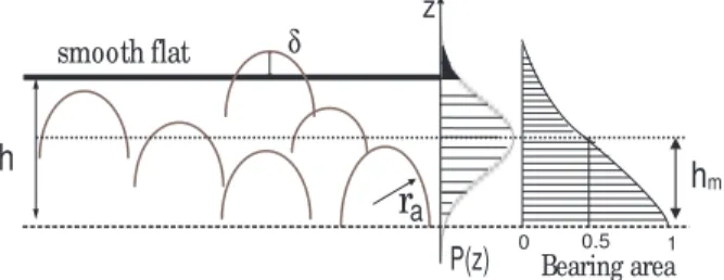
The contact between rough surfaces has been widely studied, and various statistical models of contact have been developed that are related to the first work of Greenwood and Williamson. Contact of two rough surfaces (standard deviation for roughness σp)
is equivalent to contact of a smooth flat surface with a rough surface having a standard deviation for roughness σ =√2σp [19, 20].
δ h smooth flat ra P(z) 0 0.5 1 hm z Bearing area
Figure 1. Contact of a rough surface with a flat one
The electrical contact resistance R between rough surfaces is the sum of the parallel microcontact resistances Ri corresponding to the ensemble of asperities in contact with
the flat one. The number of asperities on the rough surface is Na, with a Gaussian
distribution of asperity heights described by the function Ψ(z).
Ψ(z) = 1 σ√2πexp µ −(z − hm) 2 2σ2 ¶ (1)
The probability for an asperity to be in contact with the flat surface is equal to the probability that its height is greater than the plane separation h where h is the distance between the flat plane and the reference plane (cf:Eq1). If a summit height exceeds the separation h it will be compressed by δ = z − h and will give a contact area Ai = κπδra,
here ra is the radius of curvature of the asperity and κ is equal to 1 in the case of elastic
deformation and is equal to 2 in the case of fully plastic deformation. In general, even for the lowest applied forces, the metal particles deform plastically and we shall consider that κ equals 2.
The real contact area Ac between 2 particles with a separation h is then given by the integral:: Ac = 2πraNa Z ∞ h (z − h)Ψ(z)d(z) (2)
which can be written after a change of variable
Ac(h) = 2πraNa Z ∞ 0 x exp µ −(x + h − hm) 2 2σ2 ¶ dx (3)
The relationship between the real contact area and the contact load in the case of fully plastic deformation is given by [20]:
F = 2.8YsAc (4)
where Ys is the yield strength of the material.
The electrical contact resistance Rp is the sum of the constriction resistance Rc
and tunnel resistance Rt due to the presence of an insulating film. The ratio Rc/Rt
was examined for conductive particles indicating that the constriction resistance can be neglected in favor of the tunnel resistance [18]. Thus the contact resistance is the tunnel resistance given by:
Rp =
ρt
Ac
(5)
where ρt is the tunnel resistivity given in the case of low voltage (V∼= 0) and for a
rectangular barrier by Simmon’s equation [21] expressed in Ω.cm2
:
ρt(g, ϕ) = 32 × 10
−12g exp(gγ)
γ (6)
with γ = 1.024√ϕ expressed in (1/˚A), where ϕ is the height of potential barrier which can be obtained by subtracting the insulator’s work function from that of the conductor [26]. In the case of elastomer-nickel interface the value of ϕ is taken equal to 0.7 ev, g is the thickness of the insulating film between adjacent particles.
The effect of image forces, which decrease the area of the potential barrier by rounding off the corners and reducing its thickness, can be included in the formula (6).In this case the tunnel resistivity of a thin insulating film of thickness g, dielectric constant K and height of potential barrier ϕ is given by:
ρt(g, ϕ, K) = 31.6 × 10 −12∆g exp(1.024∆g√ϕL) √ϕL (7) ϕL= ϕ[1 − 11.5 gKϕ − 12ln( gKϕ 6 − 1)] (8) ∆g = g2− g1 = g − 12 k.ϕ (9)
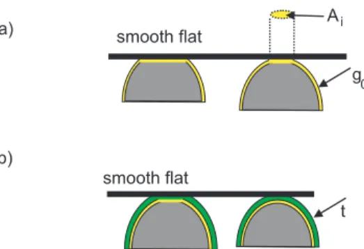
In the case of the powder alone, the thickness of the insulating film is just the one of the oxide layer g0 between particles: g = g0, whereas in the case of composites the
Figure 2. Sketch of a contact between one asperity and a flat plane in two case: (a) Powder: g0 the thickness of the oxide remains constant with pressure (b) composites:
variation of the thickness of soft layer t grafted on the surface of the asperity
thickness of the insulating film is the sum of the oxide and of the grafted polymer layer t on the surface of particles: g = g0+ t as is illustrated in Fig (2)
The oxides are much stiffer than the metal. Thus, when pressure is applied, the thickness of oxide g0 remains constant versus pressure. Therefore, for powder, g = g0
which means that ρt is constant, so from relation (5), the change of resistance is only
due to the increase of contact area with pressure. From Eqs (5) and (4), the contact resistance of compressed powder versus applied force follows a power law as:
R = 2.8ρt(g0)Ys
F (10)
But in the case of composites, both numerator and denominator of the equation (5) change with pressure: we have a change of ρtdue to the variation of the thickness of the
soft layer t and, as before, we have a variation of contact area Ac. Under pressure, the
interparticle separation changes from h0 (separation at zero pressure) to h and also the
thickness of soft layer changes from t0 to t. If ǫh and ǫg are respectively the deformation
of the average asperity height between two particles and the deformation of the soft layer, we can write:
(
h = h0(1 − ǫh)
t = t0(1 − ǫg)
However, both ǫh and ǫg are unknown; they must be expressed in terms of
macroscopic experimental deformation ǫ. In these expressions the deformations are counted as positive numbers; ǫh = h0 − h/h0, ǫg = t0 − t/t0. Assuming that,during
the compression, only the layer composed of the asperities and polymer is deformable, keeping constant the mean diameter d of particles, ǫh is given by:
ǫh = d + h0 h0 ǫ ≈ d h0 ǫ (11) Thus we have: h h0 = (1 − d h0 ǫ) (12)
We call Eh the modulus of the layer of thickness h formed by the mixture of
asperities and polymer and Eg the modulus of the thin polymer layer between two
asperities. The equality of stress imposes that: Ehǫh = Egǫg hence ǫg = Eh Eg d h0 ǫ (13)
In the lubrication approximation, the modulus Eh is related to the total modulus
E of the composite by [27]: E = 3 2φ d hEh therefore, from Eq (13): ǫg = 2 3φ h h0 E Eg ǫ (14)
and finally using Eq(12) we obtain:
ǫg = λ(1 − d h0 ǫ)ǫ (15) where λ = 2 3φ E Eg (16)
To summarize we find that h and t can be expressed in terms of the macroscopic strain ǫ as: h = h0(1 − d h0ǫ) t = t0[1 − λ(1 − d h0ǫ)ǫ]
Putting this expression for h in Eq (3) , the contact area becomes :
Ac(ǫ) = 2πraNa Z ∞ 0 x exp − (x + h0(1 − d h0ǫ) − hm) 2 2σ2 dx (17)
For the change of tunnel resistivity with the the thickness t of the polymer layer we use the simpler form Eq(6) of the tunnel resistivity:
ρt= 32 × 10 −12(g0+ t) exp(γ(g0+ t)) γ = 32 × 10−12g0+ t g0 g0 γ exp(γg0) exp(γt) = ρt(g0) g0+ t g0 exp(γt)
ρt(ǫ) = ρt(g0) g0+ t0[1 − λ(1 − d h0ǫ)ǫ] g0 exp[γt0(1 − λ(1 − d h0 ǫ)ǫ)] (18)
In Eq (17) ra, Na, σ and hmare the parameters of roughness given by AFM technique
(see table 1). The initial separation h0 between the two average planes-corresponding to
a bearing area of 0.5- is simply equal to 2hm in the case of particles slightly in contact.
Nevrtheless if initially the particles were pressed against each other then h0 would be a
parameter. The function ρt(g0) is given by Eq (7).
The MRE composite is formed by a number Nch of conductor paths binding the
two macroscopic electrodes, and each path contains M particles, so the total resistance of composite is given by [11]: R = (M/N )Rp. By introducing the volume fraction φ,
the total resistivity of composite ρc is:
ρc = π 6 d φ ρt Ac (19)
with ρt given by (18) and Ac(ǫ) by Eq (17) ; d is the mean diameter of particles.
The parameters of the model are g0, t0 and λ. The first one, g0, is the thickness
of the oxide layer which will be determine in the next section by measurement of the piezoresistivity of the powder. The second one,t0, is the remaining thickness of the
polymer layer between two asperities which are just entering into contact, the third one, λ, is related to the compression of the polymer layer. Its value will be determined from the fit of the model and compared with its estimated value given by Eq(16) where E is determined from the experimental stress-strain curves of composite and Eg is taken
from the stress-strain curve of the polymer alone without fillers. In subsection 4.2 the theoretical value of λ will be compared with the result of the fit.
3. Sample characterization
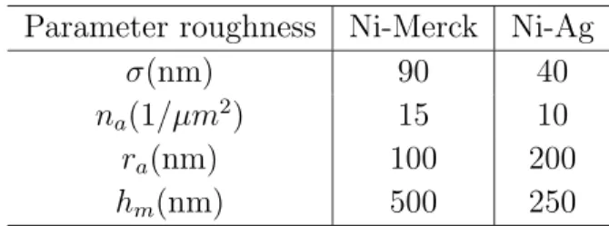
We have used two kinds of metal powder: nickel powder produced by Merck KgaA(Ni-Merck) and silver coated nickel particles (Ni-Ag) from Novamet corporation, with 15 % weight in proportion of silver which corresponds to about 0.47 µm of thickness. The average size of these two kinds of particles was about the same: 10µm. Both Ni-Merck and Ni-Ag are spherical with a rough surface Fig (3). The roughness is characterized with help of an AFM, the table (1) summarizes the parameters with σp the root mean
square of the height distribution, na is the density of summits (the number of local
maximums per unit area in µm2
), ra is the average radius of curvature of the asperities
and hm is the height of the plane corresponding to a half bearing area Fig (1); the
software gives the bearing area curve after removing the average curvature of the surface. The area where the asperities can come into contact depend on the radius of the particles compared to hm and can be obtained by using the Gaussian probability function Eq(1)
for the height of the asperities; for a diameter of 10µm we obtain a surface of 2µm2
for Ni-Ag and 2.7µm2
Parameter roughness Ni-Merck Ni-Ag σ(nm) 90 40 na(1/µm 2 ) 15 10 ra(nm) 100 200 hm(nm) 500 250
Table 1. Roughness parameters of nickel powder
The polymer used to make a MRE composite is the silicone RTV141A associated to RTV141B hardener from Rhodia. The powder is carefully mixed with the monomer, initially by hand and then in a mixer during 1 hour to break the maximum of the aggregates and to homogenize the mixture. This mixture was degassed under vacuum during 15 minutes to eliminate air bubbles and then poured into a cylindrical mold with two brass discs on each side which will be used as electrodes during measurements of resistance. The mold is placed between the poles of an electromagnet and the magnetic field is raised progressively till approximately 140 kA/m. Under the effect of this field, the particles align in the direction of magnetic field. The sides of the brass elements in contact with the sample were electroplated with nickel in order to ensure a good contact between particles and electrodes, because under a magnetic field the particles attract each other but they are also attracted by this nickel layer on the electrodes. To prevent the sedimentation of the particles the cylindrical mold was rotated during the curing process. The time of polymerization can take over 24 hours at ambient temperature but less than one hour when heating at 80◦
C. In this study the curing of composite was made at ambient temperature.
4. Experimental Results and discussion
4.1. Powder conductivity
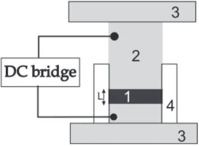
In order to get a better understanding of the piezoresistivity of these composites, we have begun by a study of the conductivity of the metal powder.The powder after being weighed, is introduced into a cylinder made of teflon (inner diameter 20 mm). A brass piston is fixed on the bottom of the cell. In the upper part of the cell, a brass plunger can slide vertically without friction with the wall of the container fig (4).
The dc electrical resistance was measured with a multimeter HP 3490A in the range of resistance from few ohms to 10 megohms. Another method known as four-probes technique was also used: the two terminal electrodes were connected to a current source and two other wires measured the voltage drop across sample. The main advantages of four-probes technique are to allow measurements of low resistances and also to change the intensity of the current in order to be sure that the powder exhibits a ohmic behavior. The pressure was applied on the sample by means of a Dynamic mechanical Analyser (VA450+) from Metravib fig (5): this device being equipped with capacitive
displacement sensor and force sensor in the range 0 to 450 N.
(a) Ni-Ag powder (b) Ni-Merck powder
Figure 3. Scanning electron microscopy of the two powders
Figure 4. Experimental device used for measurement of electrical resistance of powder with applied pressure: (1) powder, (2) brass piston, (3) holders, (4) insulating cylinder
Sample
Force sensor
Figure 5. Viscoanalyseur
Before rising the pressure on the powder, and just under the weight of the piston (0.3kPa) the resistivity is about 108
for Ni-Merck powder and 104
for Ag powder. Ni-Ag powder is more conductive than the Ni-Merck, this difference is due to the difference in oxide layer thickness on each type of particles.
The volume fraction of the powder is obtained by: φ = ρa
ρp
ρa is the apparent density of powder, and ρp is the density of nickel particle: 8.9
g/cm3
The volume fraction was 0.42 for Ni-Ag powder and 0.40 for Ni-Merck powder. These values are far from 0.64 for random packing of monodisperse spherical particles; it means that, due to the roughness of the particles, we have a loose packing with a lower coordination number than for a dense random packing
The stress-strain curves and pressure dependence of electrical resistance for nickel powders are presented in Fig (6) to (9)
0 0.005 0.01 0.015 0.02 0.025 0.03 0 1 2 3 4 5 6 7 8 9 10 Strain Stress
Figure 6. Stress-strain curve of Ni-Ag powder
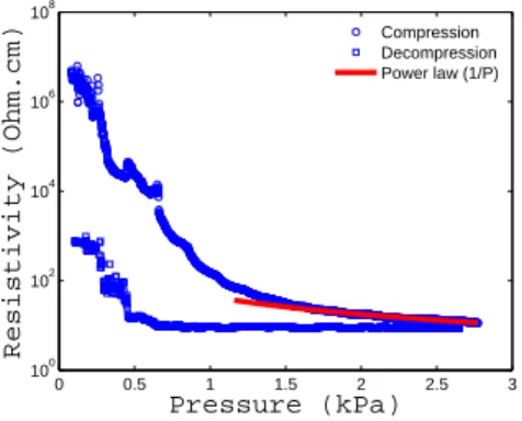
0 0.5 1 1.5 2 2.5 3 100 102 104 106 108 Pressure (kPa) Resistivity (Ohm.cm) Compression Decompression Power law (1/P)
Figure 7. The pressure dependence of electrical resistivity of NiAg powder,the solid line is a fit with Eq( 10)
During the compression of the Ni-Ag powder, there are two distinct intervals on the stress-strain curve, the first interval corresponds to a slight increase in pressure until 1.5 kPa, and a large increase of the strain Fig (6), and at the same time, the resistivity falls from a few megohm.cm to a few ten ohm.cm Fig (7). The high value of initial resistivity suggested that there are few contacts between asperities with a small contact area because the powder is not compacted and poorly organized in the cell. When pressure is applied the particles rearrange and fill the empty space and also increase their contact surface, hence the large increase of the deformation and the decrease of resistivity. In the second interval, a large increase in pressure -between 1.5 and 8 kPa-is recorded together with a low deformation from 0.02 to 0.028 and a small decrease of resistivity from 40 to 10 Ohm.cm. In this interval, the deformation recorded is due only
to the deformation of the asperities and not to their rearrangement; also the decrease of the resistance comes only from the increase of the contact area. It is worth noting that we observe an important hysteresis on the stress strain curve during decompression because the particles remain compacted after unloading which is also well confirmed by the non-return of resistivity to it’s initial value Fig (7).
0 0.005 0.01 0.015 0.02 0.025 0 20 40 60 80 Strain Stress (kPa)
Figure 8. Stress-strain curve of Ni-Merck powder
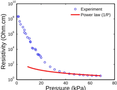
0 20 40 60 80 100 102 104 106 108 1010 Pressure (kPa) Resistivity (Ohm.cm) Experiment Power law (1/P)
Figure 9. The pressure dependence of electrical resistance of Ni-Merck powder; the solid line is a fit with Eq( 10)
The mechanical Fig (8) and electrical Fig (9) behavior of the Ni-Merck powder are similar Ni-Ag powder, the only difference is the sensitivity to pressure. The Ni-Merck powder must be compressed ten times more than the Ni-Ag powder in order to get the same value of resistance. This difference in resistivity is explained by a larger thickness of the oxide layer in Ni-Merck powder than in Ni-Ag powder.
Both for Ni-Ag powder and Ni-Merck powders, at the end of the compression, the piezoresistivity follows a power law with pressure P with a coefficient close to (-1), this behavior is described by the model Eq (10). Knowing the yield strength Ys (200 MPa
for silver, and 300 MPa for nickel) and using the tunnel resistivity ρt(g0) given by Eq(7)
4.2. MRE composite conductivity
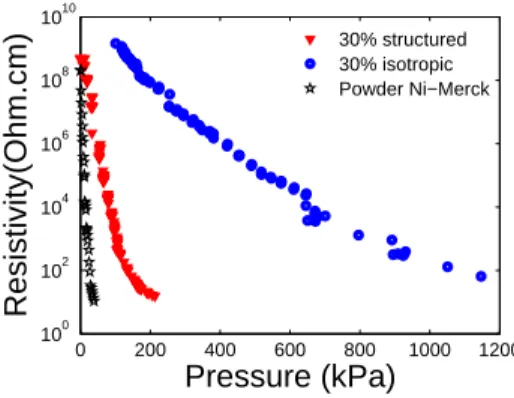
In Fig(10) we have compared the piezoresistivity of MRE composite where the particles are aligned in the direction of the applied magnetic field to the one of an isotropic composite at the same volume fraction. We have also added on the same figure the piezoresistivity of the powder; as already told the drop of resistance with pressure is larger for the powder, but it is not reproducible since, after releasing the compression, the resistance does not come back to its initial value contrary to the elastomer based composite. On the other hand, comparing the isotropic and structured composite we see that there is an order of magnitude of pressure sensitivity in favor of the structured one. The reason is that the magnetic force, during structuration, brings particles in closer contact, whereas in the isotropic composite the separation between the surfaces of neighbor particles and the connectivity depend mainly on the volume fraction of fillers. The larger sensitivity to the pressure in powder compared to the MRE composite is due to the presence of the polymer which rises the rigidity of the composite, so more pressure is needed for the composite to get the same drop of resistance.
0 200 400 600 800 1000 1200 100 102 104 106 108 1010 Pressure (kPa) Resistivity(Ohm.cm) 30% structured 30% isotropic Powder Ni−Merck
Figure 10. Piezoresistivity of structured and isotropic composites Ni-Merck compared to the first compression of powder
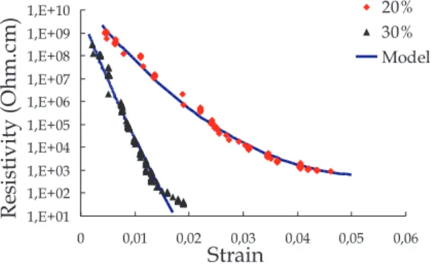
Figs (11) and (12) shows the experimental results for the piezoresistivity of MRE composites NiMerck and NiAg compared to the prediction of the model Eqs (17) -(19). The thickness of oxide layer of each particles founded in the case of a dry powder is used in order to calculate ρ(g0).
The table 2 summarizes the parameters needed for the best fit of the model. h0
is the initial mean separation distance between two adjacent particles. We can note that h0 is slightly smaller than 2hm (cf. table1); it is rather expected since the effect
of the applied magnetic field before curing is to bring particles in closer contact. The average thickness of the remaining insulating film, t0, is two times less in composite
Ni-Ag than in composite Ni-Merck; this is perhaps related to a larger adsorption energy of the polymer with Ni than with Ag. The initial modulus Eg of the elastomer itself
stress-strain curves of Fig(13). Hence from Eq(16) the value of the parameter λ can be calculated and compared to the values obtained from the fit of piezoresistivity curves. The agreement is quite reasonable (cf. table2) except for the volume fraction of 30% Ni-Merck where the value from the fit is about 3 times larger than the estimate. This discrepancy means that he model is likely less valid at high volume fraction. This is visible in Fig (11) where the fit for 30% is not as good as the other ones. We have used an hypothesis of an ideal structure composed of independent chains of particles which is certainly less and less true when the volume fraction of fillers increases, because the alignment of particles under magnetic field is only well formed at low volume fraction. If we put apart this high volume fraction it is noticeable that this piezoresistivity model is able to reproduce the decrease of resistance with strain with only one parameter which is the the initial thickness of the interfacial polymer layer (the initial distance h0 gives
the initial resistance at zero strain).
Figure 11. Piezoresistivity of MRE composite Ni-Merck for two volume fractions; solid line is the model from Eq(19)
Figure 12. Piezoresistivity of MRE composite Ni-Ag ; solid line is the model from Eq(19)
Composite h0 (nm) t0(˚A) E (Mpa) λ fit λ (Eq16)
Ni-Ag (5%) 480 10 0.7 15 14 Ni-Ag (10%) 380 9 1 9 11 Ni-Merck (20%) 905 20 4 25 20 Ni-Merck (30%) 900 20 8 80 30
Table 2. Parameters fits include in the model (19)
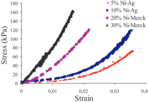
Figure 13. Stress-strain of MRE Ni-Merck and MER Ni-Ag
5. Conclusion
Some field structured composites have been synthesized from two kinds of magnetic particles: nickel and nickel coated with silver, dispersed in a silicone polymer. The roughness of these two types of particles was characterized with the help of an atomic force microscope. A model based on the tunnel resistance of microcontacts between the asperities was developed with the area of contact given by plastic deformation of asperities whose height distribution was represented by a Gaussian probability function. The two parameters of this model were the thickness of the oxide layer and the thickness of the polymer layer squeezed between two asperities. The first parameter was deduced from the fit of the resistivity versus pressure of the powders at high pressure. Then the resistivity of the composite versus pressure was measured for two different volume fractions and for the two types of particles. The thickness of the polymer layer between two asperities before they get deformed was deduced from a fit of the experimental curves and was shown to be in the range of 10 ˚A to 20 ˚A. The shrinkage of this polymer layer under applied pressure is well represented by a simple model based on the hypothesis that in field structured composites the local deformation is the macroscopic one amplified by the factor d/h0 where d is the average diameter and h0 the distance between the two
average surfaces. Unlike the powder, after a cycle of compression decompression the resistance comes back to its initial value and next cycles show no hysteresis; it is also worth noting that our experiments have shown that the sensitivity to pressure of a field structured composite was about ten times larger than the one of a usual composite.
Future research should be directed toward the inclusion of smaller particles with higher magnetic saturation like, for instance, nanoparticles of cobalt. It would likely improve the durability and the reproducibility of the piezoresistivity of these composites when cycled during a long time which is important for the use of these materials as pressure sensors.
References
[1] Bhattacharya S K 1992 Metal Filled Polymers (New York: Marcel-Dekker)
[2] Fulton J A, Moore R C, Lambert W R and Mottine J J 1989 Proc. 39th Electronic Components Conf. IEEE. 3971
[3] Carmona F and Mouney C J 1992 Mater. Sci. 27 5
[4] Feller J F, Linossier I and Grohens Y 2002 Mat. Lett. 57 64 [5] Barkauskas J 1997 Talanta. 44 1107
[6] Kim Y S, Ha S C, Yang Y, Kim Y J, Cho S M, Yang H and Kim Y T 2005Sens. Actuators. B. 108285
[7] Jin S, Mottine J, John J and Sherwood R C 1987 U.S. Patent. 4,644,101 [8] Kirkpatrick S 1973 Rev. Mod. Phys. 45 574
[9] Zallen R and Sher H 1971 Phys. Rev. B. 4 4471
[10] McLachlan D S, Blaszkiewicz M and Newnham R E 1990J. Am. Ceram. Soc. 73 2187 [11] Ruschau G R, Yoshikawa S and Newnham R E 1992J.Appl. phys. 72 953
[12] Celzard A, March J F, Payot F and Furdin G 2002 Carbon. 40 2801 [13] Holm R 1967 Electric Contacts Berlin: Springer
[14] Holm R 1950 J. Appl. Phys. 22 569
[15] Roldughin V I and Vysotskii V V 2000Progress in Organic Coatings 39 81
[16] Martin J E, Anderson R A, Odinek J, Adolf D and Williamson J 2003 Phys. Rev. 67 094207 [17] Coquelle E and Bossis G 2005 Journal of Advanced Science 17
[18] Kogut L, and Komvopoulos K 2004J. Appl. Phy. 95 576
[19] Johnson K L 1985 Contact Mechanics Cambridge University Press: Cambridge, UK [20] Zhao Y, Maietta D M and Chang L 2000 J. Tribo. 122 86
[21] Simmons J G 1963 J. Appl. Phys. 34 1793
[22] Yoshikawa S, Ota T and Newnham R 1990 J. Am. Ceram. Soc. 73 263
[23] Bloor D, Donnelly K, Hands P J,Laughlin P and Lussey D 2005 J. Phys. D: Appl. Phys. 38 2851 [24] Lundberg B and Sundqvist B 1986 J. Appl. Phys. 60 1074
[25] Ohe K and Naito Y 1971J. Appl. Phys. 10 99
[26] Zhang X W, Pan Y,Zheng Q and Yi X S 2001 Polym. Int. 50 229