HAL Id: inria-00589062
https://hal.inria.fr/inria-00589062
Submitted on 27 Apr 2011
HAL is a multi-disciplinary open access
archive for the deposit and dissemination of
sci-entific research documents, whether they are
pub-lished or not. The documents may come from
teaching and research institutions in France or
L’archive ouverte pluridisciplinaire HAL, est
destinée au dépôt et à la diffusion de documents
scientifiques de niveau recherche, publiés ou non,
émanant des établissements d’enseignement et de
recherche français ou étrangers, des laboratoires
A Subdivision Method for Computing Nearest Gcd with
Certification
Guillaume Chèze, André Galligo, Bernard Mourrain, Jean-Claude Yakoubsohn
To cite this version:
Guillaume Chèze, André Galligo, Bernard Mourrain, Jean-Claude Yakoubsohn. A Subdivision Method
for Computing Nearest Gcd with Certification. Theoretical Computer Science, Elsevier, 2011, 412 (35),
pp.4493-4503. �10.1016/j.tcs.2011.04.018�. �inria-00589062�
A Subdivision Method for Computing Nearest Gcd with
Certification
Guillaume Ch`ezea, Andr´e Galligob,c, Bernard Mourrainc, Jean-Claude Yakoubsohna aInstitut Math´ematique de Toulouse, ´equipe MIP
Universit´e Paul Sabatier 118 route de Narbonne 31062 Toulouse, France [email protected] [email protected]
bLaboratoire J.A. Dieudonn´e,
UMR CNRS 6621, Universit´e de Nice Sophia-Antipolis, Parc Valrose, 06108 Nice Cedex 02
[email protected] cGALAAD, INRIA M´editerran´ee
2004 route des Lucioles BP 93, 06902 Sophia Antioplis
France
Abstract
A new subdivision method for computing the nearest univariate gcd is described and analyzed. It is based on an exclusion test and an inclusion test. The exclusion test in a cell exploits Taylor expansion of the polynomial at the center of the cell. The inclusion test uses Smale’s
α-theorems to certify the existence and unicity of a solution in a cell.
Under the condition of simple roots for the distance minimization problem, we analyze the complexity of the algorithm in terms of a condition number, which is the inverse of the distance to the set of degenerate systems.
We report on some experimentation on representative examples to illustrate the behavior of the algorithm.
1. Introduction
Computing an approximate gcd of two polynomials is a fundamental and difficult problem in symbolic-numeric computation. It has been extensively studied in the Computer Algebra community, following different strategies: [6, 22, 19, 8, 13, 11, 2, 10, 3, 4, 20, 26, 15, 14, 18, 24]. . . . The problem is usually formulated as finding a perturbation of a pair of polynomials (f, g) within a given ball of radius ε, such that the perturbed pair (p, q) has a non-trivial exact gcd (of highest possible degree) in this ball.
In our approach, we reformulate the problem as an optimization problem: Given the poly-nomial pair (f, g) of a given degree, we look at the nearest polypoly-nomial pair (p, q) of the same degree which has a non-trivial exact gcd. The ε-approximate gcd problem has a solution iff this nearest pair with a non-trivial gcd is within a distance ε.
This paper is an extended version of the conference paper [7]. In the first section, we present the optimization problem that we are going to solve, we state our complexity main
result and mention the related approaches in the literature for approximate gcd computation. In section 2, we describe the main ingredients of our subdivision method. In section 3, we analyze its complexity using α-theory. Finally, in section 4, we report of some experimentation to illustrate the behavior of the algorithm.
1.1. A minimization problem
As usual, we denote by Rd[z] and Cd[z] the vector spaces of univariate polynomials of degree
less or equal to d, with coefficients in R and C. We denote by f = (f0, . . . , fd)T the coefficients
of the polynomial f (z) =Pdk=0fkzk∈ Rd[z]. The 2-norm of f is ||f ||2=
Pd
k=0fkf¯k.
We address the nearest gcd problem, i.e. the following minimization problem:
Problem 1.1 Given two degree d polynomials f (z) and g(z), find two degree d polynomials p(z) and q(z) with a non trivial gcd, which are solutions of the minimization problem
min p,q∈Cd[z] Resultantd(p,q)=0
||f − p||2+ ||g − q||2, (1)
Here Resultantd(p, q) is the resultant of p and q when they are considered as polynomials of
degree d. We recall that Resultantd(p, q) = 0 if and only if gcd(p, q) is non-trivial or deg (p) < d
and deg (q) < d. In the last case p and q have a common root at infinity, see Example 2 in Section4.
In our formulation of the nearest gcd problem, we look for the nearest pair (p, q) of degree at most d with a non-trivial gcd. In Example 1 in Section 4 we will see that if deg f = 7 and deg g = 8 then we can find p and q with degree 8. Thus the degree of p can be bigger than the degree of f .
N.K. Karmarkar and Y.N. Lakshman in [15] reduced that problem to another minimization problem : Problem 1.2 minz∈P(C) f (z)f (z) + g(z)g(z) Pd k=0zkzk . (2)
Moreover, a global minimum z0of (1.2) is a root of a nearest gcd and determines the polynomials
p and q of (1.1) by the formulas:
p(z) = f (z) −Pdf (z0) k=0z0kzk0 d X k=0 z0kzk q(z) = g(z) −Pdg(z0) k=0z0kz0k d X k=0 z0kzk.
We observe that with the change of variables z = X + iY , the problem amounts to minimize a homogeneous rational bivariate function
F(z) = F (X, Y ) = N (X, Y ) D(X, Y ).
1.2. Notations
We denote by G(X, Y ) = (G1(X, Y ), G2(X, Y )) the couple of numerators of the gradient
∇F (X, Y ). We denote by Pµ= N − µD where µ ∈ R and F = ND.
For G(X, Y ) = (G1(X, Y ), G2(X, Y )) with Gk(X, Y ) = deg GXk l=0 X i+j=l Gk;i,jXiYj∈ C[X, Y ], k = 1, 2,
we define the (Bombieri) norm kGkB by:
kGk2 B = X k=1,2 deg GXk l=0 X i+j=l Gk;i,jGk;i,j i!j! deg Gk! .
AF := {(xi, yi) | i = 1, .., n } is the set of global minima of F (X, Y ). We assume that this
set is finite.
ZH is the set of zeroes of a polynomial function H(X, Y ) and d(x, y, ZH) is the Euclidean
distance from (x, y) ∈ R2 to Z
H. The function H(X, Y ) will be specialized to Pµ(X, Y ) or to
Gi(X, Y ), i = 1, 2.
Let S or S(x, y, r) be a square centered at (x, y) and of radius r.
1.3. Our approach
We use a bisection algorithm, based on an exclusion test and an inclusion test (see below), applied simultaneously to:
1- the polynomial Pµ(X, Y ) = N (X, Y ) − µD(X, Y ) 2- the system G(X, Y ) = (G1(X, Y ), G2(X, Y )).
Our bisection algorithm will iteratively update a list of retained squares and a list of ap-proximate global minima of F . We prove a complexity result in Section3.
We use G1 and G2 to compute local extrema. The polynomial Pµ is used to exclude “bad”
squares. Indeed, during our algorithm µ is a candidate for the minimum of F and we set
µ = N (x0, y0)/D(x0, y0) where (x0, y0) is a center of a square. Thus, if Pµ(x, y) > 0 in a square
S then F (x, y) > µ, and we cannot find a global minimum in S.
We follow the approach initiated by S. Smale and his co-worker in a series of papers (see e.g. [5] and the references therein) relying on their celebrated α and γ-theorems.
In section2we will briefly review some of these notions and recall the definitions of α, β, γ, we also set γ(G, AF) := max(x,y)∈AF γ(G; x, y). After that, we provide a precise quantitative
definition for a point (x, y) to be, in our setting, an approximate global minimum of F (x, y). Then thanks to the γ−theorem, the approximation is sufficiently good to imply that a Newton iteration converges quadratically towards a global minimum.
To state our result on the complexity analysis of the subdivision method, we need the following notations:
• σF := min 1
(x,y)∈AFdF(DG(x,y),Σ) where dF is the Frobenius distance and Σ is the set of
singular matrices.
• N is the maximal number of connected components of U² := V²(G1) ∩ V²(G2), for all
² > 0;
• for all ² > 0, ² K is bounding the radius of a connected component of U².
• J (G, F, r0) :=
l
log2(K r0γ(G,AF)
δ0 )
m
where r0> 0 and δ0is the smallest positive root of
(13 − 3√17) (2u2− 4u + 1)2− 4u = 0.
Theorem 1.3 (Global minimum) Assume that all the elements of AF are regular points of
the system G(x, y) = 0 and are contained in some square S0:= S(x0, y0, r0).
Denote by Rj the set of retained squares at step j. Then, for j ≥ J = J (G, F, r0), all the points
of Rj are approximate global minima of F (x, y). That is to say the Newton iteration applied to
G from a point in Rj converges quadratically to a global minimum of F .
Theorem 1.4 (Complexity analysis) For the same notations and assumptions as in above theorem, we have the following properties:
1- The number of exclusion tests is bounded by 1 + J N K2. 2- When d tends to infinity, J belongs to O
³
d log(r0) + log(σF) + log(||G||B) + log(K) +
log(d)´. The number of exclusions steps belongs to O³N K2(d log(r
0)+log(σF)+log K + log(||G||B)) ´ . Remark: 1. σF = min 1
(x,y)∈AFdF(DG(x,y),Σ) is related to the condition number of the system. That is
why we keep this constant in the big O notation.
Unfortunately, we do not know how to bound this constant in terms of the degree of f and g. The computation of this kind of bound is a difficult problem.
1. ]AF ≤
X
(p,q) solution of Problem1.1
deg gcd(p, q).
Thus if Problem1.1has a unique solution then ]AF ≤ deg gcd(p, q) ≤ d.
2. In this paper, in order to apply α and γ−theorems, we suppose that all the elements of
AF are regular points of the system G(x, y) = 0. We could avoid this hypothesis, instead
of using α and γ−theorems, by relying on the tools developed in [12].
1.4. Other approaches in the literature
The nearest GCD problem has been studied with different approaches and with other for-mulations by many authors.
1.4.1. Algebraic approach via Euclid’s algorithm, resultant and subresultant
The first papers, see for example Brown [6], on the complexity of Euclid’s algorithm only works with exact coefficients. Then the numerical case has been successively considered by Sch¨onhage [22], Noda and Sasaki [19], Corless, Gianni, Trager and Watt [8], Hribernig and Stetter [13], Emiris, Galligo and Lombardi [11], Beckermann, Labahn [2]. These authors con-sider the so-called near GCD or the ²-GCD problem. The singular value decomposition was first applied to the Sylvester matrix, in [8], and later applied to the subresultant matrices, in [10,11] in order to get a certification when a condition (depending on the level of accuracy) is satisfied. An efficient implementation is done in [21].
1.4.2. Pad´e approximation and structured matrices approach
See the book of Bini and Pan [3] and the bibliography therein, and more recently Boito, Bini [4].
1.4.3. Rootfinding and cluster root approach
Pan [20] and, more recently, Zeng [26] use root finding and least squares methods.
1.4.4. Optimization approach
The resolution of problem1.2is the main and the most “time-consuming” step of the method propose in [15] that we aim to improve. The authors rely on techniques from Arnon-McCallum [1] and Manocha-Demmel [16]. The second paper is based on resultant for expressing the in-tersection of two curves and on numerical computation of eigenvalues and eigenvectors by QR iterations. Therefore the expected running time is in O(p3) where p is the product of degrees
of two curves, hence the complexity of the algorithm is at least in O(d6).
Kaltofen and his co-workers [14] determine approximate GCDs from methods based on structured total least square (STLN). The STLN is an iterative method of the family of Gauss-Newton methods. The authors describe its application to the case of the Sylvester matrix associated to the input polynomials f and g, then show its interest and efficiency by producing the results of experiments. However, since the starting point of their Gauss-Newton like method is not precised, the method can diverge. This is an important drawback.
Nie-Demmel-Gu [18] uses a sum of squares (SOS) technique, the resolution relies on semi definite programming (SDP). For the nearest GCD problem, this yields linear matrix inequal-ities (LMI) whose size s is O((d + 2)(d + 1)) whose complexity of resolution by projective algorithm is in O(s3) [17]. So, one ends up with a complexity in O(d6).
More recently, Terui [24] uses a generalization of the gradient-projection method proposed by Tanabe [25]. Then he obtains a fast algorithm for solving a constrained minimization problem related to the approximate gcd problem. Unfortunately, there exists no complexity results for this approach. Furthermore, in this method the degree of the approximate gcd is given in input.
2. The proposed bisection method
2.1. Principles
We propose a bisection method, described below, to approximate the global minima of the function F (X, Y ) defined in the introduction. In the next section, a procedure for computing an
initial square is given ; so we suppose here that a square S(x0, y0, r0) containing all the global
minima is known.
The bisection method is based on an exclusion test and an inclusion test. An exclusion test, denoted hereafter by E(F, S) or E+(F, S), is defined on the set of squares and returns true if
the function F has no zero in the square S or false if it might have a zero. Examples of exclusion tests are provided in section3.
An inclusion test I(G, S) is needed to numerically prove the existence of a local minimum: it takes G = (G1, G2) and a square S then returns true if there exists a ball B(x∗, y∗, r∗),
containing S, which contains one zero of G, in that case it also returns (x∗, y∗, r∗), otherwise it
returns false.
Our definition of approximate minima is based on γ-theorem and α-theorem of Smale [23], [5], [12], applied to the system G(x, y). We first introduce some quantities and the corre-sponding classical notations:
• β := β(G; x, y) = ||DG(x, y)−1G(x, y)|| • γ := γ(G; x, y) = supk≥2 `1 k!||DG(x, y) −1DkG(x, y)||´1/(k−1) • α := α(G; x, y) = βγ.
• γ(G; AF) = max(x,y)∈AFγ(G; x, y).
Smale’s γ−theorem [5] states:
Theorem 2.1 Let (x∗, y∗) be a zero of G and suppose that DG(x∗, y∗) is invertible. If
k(x, y) − (x∗, y∗)kγ(G, x∗, y∗) ≤ 3 −
√
7 2
then the Newton iteration from (x, y) converges quadratically to (x∗, y∗).
This leads to the following definition and quantitative results on the convergence of Newton scheme.
Definition 2.2 The point (x, y) is an approximate global minimum of F (x, y) if
d((x, y), AF) ≤ 3 −
√
7 2γ(G, AF).
Under this condition, the γ−theorem asserts that the Newton iteration from any point in the ball B(x∗, y∗, 3−√7
2γ(G,AF)) where (x
∗, y∗) ∈ A
F, converges quadratically towards (x∗, y∗).
The following result gives a sufficient condition for a point to be a good starting point for the Newton iteration. This result is called α-theorem.
Theorem 2.3 If α < (13 − 3√17)/4 then G has one and only one zero in the open ball
B(x, y, σ(x, y)) with σ(x, y) =1 + α − √ 1 − 6α + α2 4γ ≤ 2 −√2 2γ .
and the Newton iteration from (x, y) converges to (x∗, y∗). Furthermore, we have
k(x∗, y∗) − Nk G(x, y)k ≤ 5 −√17 4γ ³ 1 2 ´2k−1 , where Nk
G(x, y) is the k-th iterate of the Newton iteration applied to G with starting point (x, y).
The following result gives a radius r∗ of a ball centered in (x∗, y∗) such that every point in
B(x∗, y∗, r∗) satisfies the hypothesis of the α-theorem.
Proposition 2.4 Let (x∗, y∗) be a zero of G and suppose that DG(x∗, y∗) is invertible. Let δ
0
be the smallest positive root of u −13 − 3 √ 17 4 Ψ(u) 2, where Ψ(u) = 2u2− 4u + 1. If k(x, y) − (x∗, y∗)kγ(G, x∗, y∗) ≤ δ0 then α(G, x, y) ≤ 13 − 3 √ 17 4 .
Remark: 0.07 ≤ δ0≤ 0.08.
Proof. We use the following inequality, see [23]
α(G, x, y) ≤ u
Ψ(u)2,
where u = k(x, y) − (x∗, y∗)kγ(G, x∗, y∗). Furthermore, we have u/Ψ(u)2≤ (13 − 3√17)/4 for
u ∈ [0; δ0] and this gives the desired result.
In our complexity study we will need a bound on γ(G, AF). The following proposition will
be useful.
Proposition 2.5 Let deg G = max(deg G1, deg G2), (x, y) ∈ S(0, 0, r0), Then
γ(G; x, y) ≤ kGkBkDG(x, y)−1k(deg G)2(1 + 2r02)(deg G−2)/2.
Proof. We set some notations: k(x, y)k1= (1 + x2+ y2)1/2, ∆(ai) is the diagonal matrix with
coefficients ai.
By [23, Proposition 3], we have the following bound:
γ(G; x, y) ≤ C(G; x, y)deg G
3/2
2k(x, y)k1 ,
where C(G; x, y) = kGkBkDG(x, y)−1∆(deg (Gi)1/2k(x, y)kdeg G1 i−1)k.
We use the following classical inequality kABk ≤ kAkkBk to conclude.
Let a threshold ² > 0 be given, the output of this bisection method will be a set (eventually empty) Z = {(x∗
i, yi∗, r∗i, µ∗i)}, such that : 1- the (x∗
i, yi∗)’s are approximate global minima of F (x, y) and µ∗i = F (x∗i, y∗i). 2- the ball B(x∗
i, yi∗, r∗i) contains one and only one zero of G(x, y) where ri∗= σ(x∗i, y∗i). 3- If i 6= j then B(x∗
j, yj∗, rj∗) ∩ B(x∗i, yi∗, r∗i) = ∅ and |µ∗i − µ∗j| < ².
2.2. Computation of an initial square
Lemma 1 in [15] gives us a bound for the initial square:
Lemma 2.6 Let f =Pd1
k=0fkzk, g =
Pd2
k=0gkzk, where fd1 6= 0 and gd2 6= 0. Let F be the
rational bivariate function corresponding to the approximate gcd problem. Let (x, y) ∈ AF then
k(x, y)k ≤ 5 max³ kfk 2 f2 d1 ,kgk 2 g2 d2 ´ . 2.3. Sketch of algorithm
The algorithm consists of an initialization followed by a while loop with an internal for loop. We call step k, the k-th step of the while loop.
Proposition 2.7 Assume there exists ² > 0 such that for all square S(x, y, ²) ⊂ S0 we have : 1- the inclusion test is true if S(x, y, ²) contains a zero of G.
2- the exclusion test is true if S(x, y, ²) does not contain a zero of G. Then we have :
Algorithm 2.1: Approximate gcd
Input: F = N/D, G = (G1, G2), an initial square S0 and a threshold ² > 0, as described
above.
¦ Create a set of squares L := {S0}, a set of solutions Z := ∞ and a value (the minimum
to be updated) µ := F(∞).
¦ While L is not empty do
• Compute δ = minF (xi, yi) where the (xi, yi)’s are the centers of squares of L.
• If δ < µ then µ := δ.
• For each square S of L perform the exclusion tests E+(P
µ, S), E(G1, S) and E(G2, S).
If at least one of these exclusion tests is true then remove S from L ; else, perform an inclusion test I(G, S).
• If it returns false then divide S in 4 equal squares ;
else an approximate local minimum (x∗, y∗) is provided, it is the unique zero of G(x, y)
in the ball B(x∗, y∗, r∗).
– If µ∗= F (x∗, y∗) > µ + ² then remove S ;
else update the set Z as follows:
∗ If µ∗= F (x∗, y∗) < µ then put µ := µ∗. For each element (x∗
i, yi∗, r∗i, µ∗i) of Z
do
· If µ < µ∗
i and |µ − µ∗i| > ² then remove the solution (x∗i, yi∗, r∗i, µ∗i) from Z ;
· If for any element (x∗
i, yi∗, r∗i, µi∗) of Z, |µ − µ∗i| < ² and (x∗, y∗) is not in
the ball B(x∗
i, y∗i, r∗i) then add (x∗, y∗, r∗, µ∗) to Z.
1- The algorithm stops.
2- Let µ(²) be the value of µ at the end of the algorithm with input ². Then lim²→0µ(²) =
min(x,y)∈S0F (x, y).
Proof. The point 1 holds by construction under these assumptions. For point 2, the radius
r(²) of the retained squares in the last iteration decreases. Hence from the continuity of F , we
obtain lim²→0µ(²) = min(x,y)∈S0F (x, y).
3. Complexity analysis
3.1. Exclusion test
Let H be a polynomial in R[X, Y ] and denote by DkH(x, y) the homogeneous part of degree
k of the Taylor expansion of H at the point (x, y).
Let S(x0, y0, r0) be a square. To define an exclusion function E(H, S), we rely on the
following expression and lemma:
MH(x0, y0, r0) = |H(x0, y0)| − X k≥1 ||DkH(x 0, y0)|| k! r k 0.
Lemma 3.1 If MH(x0, y0, r0) > 0 then the closed square ¯S(x0, y0, r0) does not contain any
zero of the polynomial H(x, y).
Proof. The proof follows from Taylor formula and a simple inequality.
A key to analyze the complexity of the algorithm of section2is the following lemma, see [9].
Lemma 3.2 Let H ∈ R[X, Y ] be a polynomial of degree e, consider the associated algebraic variety ZH= {(x, y) ∈ R2 : H(x, y) = 0}.
Let Le=2
1/e− 1
√
2 and mH(x, y) be the function implicitly defined by
MH(x, y, mH(x, y)) = 0.
Then mH(x, y) is related to the distance d(x, y, ZH) by the following inequalities:
Le.d(x, y, ZH) ≤ mH(x, y) ≤ d(x, y, ZH).
The exclusion tests to be used for the algorithm of section2are defined for a polynomial P by:
1- E(P, S) is true if MP(x, y, r) > 0, 2- E+(P, S) is true if M
P(x, y, r) > 0 and P (x, y) > 0.
Since the degree of Pµis 2d and the degree of the Gi’s is 4d − 2, we get: if Pµ(x, y) > 0 then
mPµ(x, y) ≥ L2d.d(x, y, ZPµ) and mGi(x, y) ≥ L4d−2.d(x, y, ZGi).
Remark: deg Gi≤ 4d − 2 because the coefficient of the term of degree 4d − 1 is 2dfd2+ 2dg2d−
2df2
d− 2dg2d= 0.
Proposition 3.3 Let H(X, Y ) = Pµ(X, Y ) or H(X, Y ) = Gi(X, Y ), i = 1, 2. Let S :=
S(x, y, r). The logical relation
E(H, S) is true means mH(x, y) > r,
so S does not contain any zero and is excluded in the bisection algorithm. Otherwise E(H, S) is false means mH(x, y) ≤ r,
and S may contain zeros. In this case S will be divided into four squares each of them with a radius r/2.
3.2. Inclusion test
Our inclusion test is based on Smale’s α-theory. The test is true if :
1- α(G; x, y) < 13 − 3 √
17
4 ,
and
2- S(x, y, r) ⊂ B¡x, y, σ(x, y)¢, in other words r√2 < σ(x, y), see Theorem2.3.
3.3. Proof of theorem1.3
Consider a retained square S := S(xl, yl,2r0k) at step k. We have µ := µkand Pµ(xl, yl) ≥ 0.
If E(Pµ, S) is false and E(Gi, S) is false, it means, by Proposition 3.3, that Pµ(xl, yl) = 0
or mPµ(xl, yl) ≤
r0
2k and mGi(xl, yl) ≤
r0
2k.
From Lemma3.2, we deduce that
if Pµ(xl, yl) > 0 then L2d.d(xl, yl, ZPµ) ≤ m(xl, yl) ≤
r0
2k.
Hence if Pµ(xl, yl) > 0, then for each (x, y) ∈ S we have
d(x, y, ZPµ) ≤ ||(x, y) − (xl, yl)|| + d(xl, yl, ZP µ) ≤ σkrk
where σk= (1 + 1/L2d) and rk:= 2r0k. In the same way,
d(x, y, ZGi) ≤ ||(x, y) − (xl, yl)|| + d(xl, yl, ZGi)
≤ ωkrk, i = 1, 2.
where ωk = (1 + 1/L4d−2). For H(x, y) ∈ R[x, y] and ² > 0, let
V²(H) = {(x, y) ∈ R2, st. ∃(u, v) ∈ C2, H(u, v) = 0, d((x, y), (u, v)) < ²}.
V²(H) is called the tubular neighborhood of the solution set of H(x, y) = 0 at distance ε.
By the previous inequalities, if Pµ(xl, yl) > 0 then we have
S ⊂ Uk := Vσk(Pµ) ∩ Vωk(G1) ∩ Vωk(G2).
Notice that AF ⊂ ∩k≥0Uk. Let κkrk be half the maximal diameter of a connected component
Uk. The area of Uk is bounded by π νkκ2kr2k where νk is the number of connected components
of Uk. For k big enough, this number of connected components is the number of real roots of
When k tends to infinity, the connected components of Uktend to the real roots of G1(x, y) =
G2(x, y) = 0 with Pµ(x, y) > 0 and κk tends to
p
2 (1 + cos(α)) where α is the angle between the tangents of the curves G1(x, y) = 0 and G2(x, y) = 0, at the root. Let K bound all the
possible κk.
Let J be the first J such that K rJ ≤ δ0
γ(G, AF), then for k ≥ J, all the points of the
retained squares are approximated zeros of the set AF, by Proposition2.4 and Theorem 2.3.
An upper bound for J is given in the theorem.
3.4. Proof of theorem1.4
To compute an upper bound for the number of exclusion tests, we notice that at step k, Uk
contains the union of the kept squares (whose exclusion test is false), their number is denoted by qk. Since the area of this union is qkr2k and must be less or equal to the area of Uk, we get
qk≤ π νkδ2k≤ π N K2.
Now, let pkbe the number of excluded squares at step k. As we know the relation 4qk−1= pk+qk
with p0= 0, q0= 1 holds, the number of exclusion tests until step j is bounded by
j X k=0 pk+ qk = 1 + 4 j−1 X k=0 qk ≤ 1 + j π N K2.
The last part of Theorem 1.4 comes from Proposition 2.5 which gives: for (x, y) ∈ AF,
log γ(G; x, y) belongs to O³log³d2r4(d−1)
0 ||G||B||DG−1(x, y)|| ´ ´ or to O³log(d) + d log(r0) + log(||G||B) + log(σF) ´ . 4. Examples
Our algorithm have been implemented in Matlab 7 (we use an Intel Xeon 3 Ghz processor) and we have perform some experiments to show its behavior. Currently, our algorithm is slower than other methods (e.g. [4, 14, 24]) due to the bound on the initial square given in Lemma 2.6. Nevertheless, our algorithm is certified. In the following we give examples and timings.
4.1. Increasing the degree
We consider the following example taken from the work of D. Rupprecht [21]. In his Ph.D. thesis, he developed a technique which allowed him to certify the degree of an approximate gcd but only if the required precision ε belongs to some intervals. There are small gaps between these intervals and the numerical computation of an approximate gcd is sensitive.
In our formulation of the nearest gcd problem, we look for the nearest pair (p, q) of degree
d with a non-trivial gcd. f = (z2 − 1.001) (z2 + 1.00000001) (z3 + 2 z2 − 2.999999 z + 1) = 1.000000000000000 z7 + 2.000000000000000 z6 − 3.000998990000000 z5 +0.998000020000000 z4 − 0.998000041009990 z3 − 2.003000010020000 z2 +3.002999029029990 z − 1.001000010010000 g = (z2 − 0.999)(z2 + 1.00000003)(z4 + 3z − 1.0000002) = 1.000000000000000z8 + 0.001000030000000 z6 + 3.000000000000000 z5 −1.999000229970000 z4 + 0.003000090000000 z3 − 0.001000030200006 z2 −2.997000089910000 z + 0.999000229770006
The nearest perturbed pair (p, q) with a non-trivial gcd that we compute is: p = (0.000000001537219 + 0.000000006148875 i) z8 +(0.999999993851125 + 0.000000001537219 i) z7 +(1.999999998462781 − 0.000000006148875 i) z6 +(−3.000998983851125 − 0.000000001537219 i) z5 +(0.998000021537219 + 0.000000006148874 i) z4 +(−0.998000047158864 + 0.000000001537219 i) z3 +(−2.003000011557218 − 0.000000006148874 i z2 +(3.002999035178864 − 0.000000001537219 i) z +(−1.001000008472781 + 0.000000006148874 i) q = (1.000000000000000 + 0.000000008719619 i) z8 +(−0.000000008719619 − 0.000000000000000 i) z7 +(0.001000030000000 − 0.000000008719619 i) z6 +(3.000000008719619 + 0.000000000000000 i) z5 +(−1.999000229970001 + 0.000000008719619 i) z4 +(0.003000081280381 − 0.000000000000000 i) z3 +(−0.001000030200006 − 0.000000008719619 i) z2 +(−2.997000081190381 + 0.000000000000000 i) z +(0.999000229770005 + 0.000000008719619 i)
The order of the perturbation is 10−8 and the degree of the corresponding gcd is 1.
Note that in this example, even if f is of degree 7, we allow a perturbation of degree 8 (which is the degree of g).
4.2. Solution at infinity
Here, we show that the global minimum can be reached at infinity. We consider:
f = z2− 4z + 3,
g = z2+ 4z + 3. In this situation, we have:
F (X, Y ) = N (X, Y ) D(X, Y ) = 2
9 + 22X2+ 10Y2+ (X2+ Y2)2
1 + X2+ Y2+ (X2+ Y2)2 .
Figure1shows the graph of F . Notice that there are no global minima of F in C. Indeed, we have
lim
k(x,y)k→∞F (x, y) = F(∞) = 2,
N (X, Y ) − 2D(X, Y ) = 16 + 42X2+ 18Y2> 0.
Then the global minimum is reached at infinity.
In this situation the initial square given by Lemma 2.6 is [−130, 130]2, and our algorithm
excludes this square after 10 iterations. That is to say, the size of the smallest excluded square is 130/210. The cpu-time in this example is 0.06 seconds.
In this situation, we have F(∞) = 2. Furthermore, with z0 = ∞ and the formula recalled
in Subsection1.1, we obtain p = −4z+3 and q = 4z+3. Notice that deg (p) < 2 and deg (q) < 2. Remark: We compute F(∞) in the following way: F(∞) = Fr(0), where Fr(z) = zdeg (F)F(1/z).
Figure 1: F has no global minima in C.
4.3. Example 3
Here, we consider:
f = 9z3− 18z2+ 3z + 1,
g = −37z3+ 63z2− 30z + 3.
We illustrate the algorithm step by step. The smallest perturbation that we obtain is: p(z) = 9.059z3− 17.875z2+ 3.26z + 1.544,
q(z) = −36.916z3+ 63.174z2− 29.636z + 3.758, and the common root is z = 0.479.
Step 1. We begin in Figure2(a) with a big square and we divide it in four squares.
(a) (b) (c)
(d) (e) (f)
Figure 2: Subdivision steps
Step 2. As we cannot exclude any squares and all the inclusion tests are false we divide each square in four squares (Figure2 (b)).
During the algorithm we compute F for each center of each square. The point in the figure corresponds to the center where F is minimum. Furthermore, the value of F at this point is equal to the real number µ defined in our algorithm.
Step 3. In Figure2 (c), we cannot exclude any squares and the inclusion tests are false. Step 4. At this step, see Figure2 (d), we can exclude a lot of squares.
Step 5. In Figure2(e), we see that we can exclude a lot of squares and one inclusion test is true. So with the Newton’s method applied to G we can compute the global minima. That is to say we apply Newton’s method with the black point as a starting point and we get the red
point (on the x-axis) as the global minimum.
Step 6. In this last step, we can exclude the last squares and we find the global minimum, see Figure2 (f).
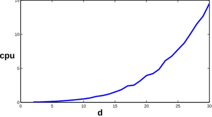
4.4. Random examples
We have carried out the following tests:
• f and g are polynomials of degree d with random coefficients. Our results are given in
Figure3, and cpu denotes the cpu-time needed in seconds to performs our algorithm.
• f (z) = (z − 1)f1(z) + 10−3²1(z), g(z) = (z − 1)g1(z) + 10−3²2(z), where f1 and f2 are
random polynomials with degree d − 1, ²1 and ²2 are random polynomials with degree
d. In these examples our algorithm gives an approximate gcd near z − 1. Our results
are given in Figure4, and cpu denotes the cpu-time needed in seconds to performs our algorithm.
Here random means that we use the Gaussian distribution with mean 0 and variance 1.
0 5 10 15 20 25 30 0 5 10 15 cpu d
Figure 3: Random examples
0 5 10 15 20 25 30 0 2 4 6 8 10 12 cpu d Figure 4: f = (z − 1).f1+ 10−3²1, g = (z − 1).g1+ 10−3²2
5. Acknowledgments
The authors thank Prof. Lihong Zhi for her comments during the presentation at SNC’09 about cases with roots at infinity (Example 2). The authors also thank the referees for their com-ments, which helped to increase the quality of the paper. B. Mourrain is partially supported by Marie-Curie Initial Training Network SAGA, [FP7/2007-2013], grant [PITN-GA-2008-214584].
[1] Dennis S. Arnon and Scott McCallum. A polynomial-time algorithm for the topological type of a real algebraic curve. J. Symbolic Comput., 5(1-2):213–236, 1988.
[2] Bernhard Beckermann and George Labahn. When are two numerical polynomials rela-tively prime? J. Symbolic Comput., 26(6):677–689, 1998. Symbolic numeric algebra for polynomials.
[3] D. Bini and V. Y. Pan. Polynomial and matrix computations, Vol 1 : Fundamental
Algo-rithms. Birkh¨auser, Boston, 1994.
[4] Dario A. Bini and Paola Boito. Structured matrix-based methods for polynomial ²-gcd: analysis and comparisons. In ISSAC 2007, pages 9–16. ACM, New York, 2007.
[5] Lenore Blum, Felipe Cucker, Mike Shub, and Steve Smale. Complexity and real computa-tion: a manifesto. Internat. J. Bifur. Chaos Appl. Sci. Engrg., 6(1):3–26, 1996.
[6] W. S. Brown. On Euclid’s algorithm and the computation of polynomial greatest common divisors. J. Assoc. Comput. Mach., 18:478–504, 1971.
[7] G. Ch`eze, J.-C. Yakoubsohn, A. Galligo, and B. Mourrain. Computing Nearest Gcd with Certification. In Symbolic-Numeric Computation (SNC’09), pages 29–34, Kyoto Japon, 08 2009. ACM New York, NY, USA.
[8] R.M. Corless, P.M. Gianni, B.M. Trager, and S.M. Watt. The singular value decomposition for polynomial systems. In A.H.M Levelt, editor, Proc. Internat. Symp. Symbolic Algebraic
Comput. (ISSAC ’95), pages 195–207, 1995.
[9] J. P. Dedieu, X. Gourdon, and J. C. Yakoubsohn. Computing the distance from a point to an algebraic hypersurface. In The mathematics of numerical analysis (Park City, UT,
1995), volume 32 of Lectures in Appl. Math., pages 285–293. Amer. Math. Soc., Providence,
RI, 1996.
[10] I.Z. Emiris, A. Galligo, and H. Lombardi. Numerical Univariate Polynomial GCD, vol-ume 32 of Lectures in Applied Math., pages 323–343. AMS, 1996.
[11] I.Z. Emiris, A. Galligo, and H. Lombardi. Certified approximate univariate GCDs. J. Pure
& Applied Algebra, Special Issue on Algorithms for Algebra, 117 & 118:229–251, May 1997.
[12] M. Giusti, G. Lecerf, B. Salvy, and J.-C. Yakoubsohn. On location and approximation of clusters of zeros of analytic functions. Found. Comput. Math., 5(3):257–311, 2005.
[13] V. Hribernig and H. J. Stetter. Detection and validation of clusters of polynomial zeros.
J. Symbolic Comput., 24(6):667–681, 1997.
[14] Erich Kaltofen, Zhengfeng Yang, and Lihong Zhi. Structured low rank approximation of a Sylvester matrix. In Symbolic-numeric computation, Trends Math., pages 69–83. Birkh¨auser, Basel, 2007.
[15] N. K. Karmarkar and Y. N. Lakshman. On approximate GCDs of univariate polynomials.
J. Symbolic Comput., 26(6):653–666, 1998. Symbolic numeric algebra for polynomials.
[16] Dinesh Manocha and James Demmel. Algorithms for intersecting parametric and algebraic curves: I simple intersections. ACM Trans. Graph., 13(1):73–100, 1994.
[17] Yurii Nesterov and Arkadii Nemirovskii. Interior-point polynomial algorithms in convex
programming, volume 13 of SIAM Studies in Applied Mathematics. Society for Industrial
and Applied Mathematics (SIAM), Philadelphia, PA, 1994.
[18] Jiawang Nie, James Demmel, and Ming Gu. Global minimization of rational functions and the nearest GCDs. J. Global Optim., 40(4):697–718, 2008.
[19] Matu-Tarow Noda and Tateaki Sasaki. Approximate GCD and its application to ill-conditioned algebraic equations. In Proceedings of the International Symposium on
Com-putational Mathematics (Matsuyama, 1990), volume 38, pages 335–351, 1991.
[20] Victor Y. Pan. Computation of approximate polynomial GCDs and an extension. Inform.
and Comput., 167(2):71–85, 2001.
[21] D. Rupprecht. El´ements de G´eom´etrie Alg´ebrique Approch´ee: ´etude du PGCD et de la
factorisation. PhD thesis, Universit´e de Nice - Sophia Antipolis, Jan. 2000.
[22] Arnold Sch¨onhage. Quasi-gcd computations. J. Complexity, 1(1):118–137, 1985.
[23] Michael Shub and Steve Smale. Complexity of B´ezout’s theorem. I. Geometric aspects. J.
Amer. Math. Soc., 6(2):459–501, 1993.
[24] Akira Terui. An Iterative Method for Calculating Approximate GCD of Univariate Poly-nomials. In ISSAC 2009, pages 351–358. ACM, New York, 2009.
[25] K. Tanabe. A geometric method in nonlinear programming. J. Optim. Theory Appl., 30(2):181–210, 1980.
[26] Zhonggang Zeng The approximate GCD of inexact polynomials. Part I: a univariate algo-rithm. Preprint 2004.