CO
2
non-LTE limb emissions in Mars’ atmosphere
as observed by OMEGA/Mars Express
A. Piccialli1, M. A. López-Valverde2, A. Määttänen3, F. González-Galindo2, J. Audouard4,5, F. Altieri6, F. Forget7, P. Drossart1, B. Gondet4, and J. P. Bibring4
1LESIA, Observatoire de Paris, CNRS, UPMC, Univ. Denis Diderot, Meudon, France,2IAA, Glorieta de la Astronomía, Granada, Spain,3Université Versailles St-Quentin; Sorbonne Universités, UPMC Univ. Paris 06; CNRS/INSU, LATMOS-IPSL, Guyancourt, France,4IAS, Orsay University, Orsay, France,5Department of Geosciences, State University of New York at Stony Brook, Stony Brook, USA,6IAPS – INAF, via del Fosso del Cavaliere, Rome, Italy,7Laboratoire de météorologie dynamique, CNRS/UPMC, Paris, France
Abstract
We report on daytime limb observations of Mars upper atmosphere acquired by the OMEGA instrument on board the European spacecraft Mars Express. The strong emission observed at 4.3 μm is interpreted as due to CO2fluorescence of solar radiation and is detected at a tangent altitude in between 60 and 110 km. The main value of OMEGA observations is that they provide simultaneously spectral information and good spatial sampling of the CO2emission. In this study we analyzed 98 dayside limbobservations spanning over more than 3 Martian years, with a very good latitudinal and longitudinal coverage. Thanks to the precise altitude sounding capabilities of OMEGA, we extracted vertical profiles of the non-local thermodynamic equilibrium (non-LTE) emission at each wavelength and we studied their dependence on several geophysical parameters, such as the solar illumination and the tangent altitude. The dependence of the non-LTE emission on solar zenith angle and altitude follows a similar behavior to that predicted by the non-LTE model. According to our non-LTE model, the tangent altitude of the peak of the CO2emission varies with the thermal structure, but the pressure level where the peak of the
emission is found remains constant at ∼0.03 ± 0.01 Pa, . This non-LTE model prediction has been corroborated by comparing SPICAM and OMEGA observations. We have shown that the seasonal variations of the altitude of constant pressure levels in SPICAM stellar occultation retrievals correlate well with the variations of the OMEGA peak emission altitudes, although the exact pressure level cannot be defined with the spectroscopy for the investigation of the characteristics of the atmosphere of Venus (SPICAM) nighttime data. Thus, observed changes in the altitude of the peak emission provide us information on the altitude of the 0.03 Pa pressure level. Since the pressure at a given altitude is dictated by the thermal structure below, the tangent altitude of the peak emission represents then an important piece of information of the atmosphere, of great value for validating general circulation models. We thus compared the altitude of OMEGA peak emission with the altitude of the 0.03 Pa level predicted by the Laboratoire de météorologie dynamique (LMD)-Mars global circulation model and found that the peak emission altitudes from OMEGA present a much larger variability than the tangent altitude of the 0.03 Pa level predicted by the general circulation model. This variability could be possibly due to unresolved atmospheric waves. Further studies using this strong CO2limb emission data are proposed.
1. Introduction
The upper atmosphere of a terrestrial planet is a region difficult to sound, both by in situ and remote sound-ing [Müller-Wodarg, 2005]. This atmospheric region is characterized by nonlocal thermodynamic equilibrium (non-LTE) that occurs when collisions between atmospheric species are not rapid enough to keep their energy levels’ populations following a known function (Boltzmann statistics). The CO2non-LTE emission at 4.3 μm in
the upper layers of the atmosphere is a good example. It is a feature common to the three terrestrial planets with an atmosphere (Venus, Earth, and Mars), and it provides a useful tool to gain insight into the atmospheric processes at these altitudes [Lopez-Puertas and Taylor, 2001]. Non-LTE emissions were first modeled in the Earth’s upper atmosphere in CO2bands at 15 and 4.3 μm [Curtis and Goody, 1956] and were later observed
on several planets in different spectral bands. Ground-based observations of CO2laser bands at 10 μm in
the atmospheres of Venus and Mars [Deming et al., 1983] were interpreted as non-LTE emissions by several
RESEARCH ARTICLE
10.1002/2015JE004981
Key Points:
• We analyzed 3 Martian years of CO2 fluorescence emission in Mars’ upper atmosphere
• Observations are mainly affected by solar illumination conditions and the altitude of the emission
• According to non-LTE model, the peak of the emission occurs at a constant pressure level of 0.03 Pa
Correspondence to:
A. Piccialli,
arianna.piccialli@obspm.fr
Citation:
Piccialli, A., M. A. López-Valverde, A. Määttänen, F. González-Galindo, J. Audouard, F. Altieri, F. Forget, P. Drossart, B. Gondet, and J. P. Bibring (2016), CO2non-LTE limb emissions in Mars’ atmosphere as observed by OMEGA/Mars Express, J. Geophys. Res. Planets,
121, doi:10.1002/2015JE004981.
Received 18 NOV 2015 Accepted 26 MAY 2016
Accepted article online 31 MAY 2016
©2016. American Geophysical Union. All Rights Reserved.
atmospheric models developed in the 1980s [Deming and Mumma, 1983]. On Jupiter, Saturn, and Titan non-LTE emissions were identified in the CH4band at 3.3 μm [Drossart et al., 1999]. More recently, the CO2
non-LTE emission at 4.3 μm was detected in the upper atmosphere of Mars and Venus by the PFS (Planetary Fourier Spectrometer) and OMEGA (Visible and Infrared Mapping Spectrometer) experiments on board the European spacecraft Mars Express (MEx) [Formisano et al., 2006; Drossart et al., 2006; López-Valverde et al., 2005] and by VIRTIS (Visible and Infrared Thermal Imaging Spectrometer) on board the European Venus Express (VEx) [Gilli et al., 2009, 2015]. These observations led to the review and extension of a comprehensive non-LTE model for the upper atmospheres of Mars and Venus [López-Valverde et al., 2005, 2011]. According to these models, during daytime the solar radiation in several near-IR bands from 1 to 5 μm produces enhanced state populations of many CO2vibrational levels which either reemit in the same wavelength (solar fluorescence) or cascade down to lower states emitting photons in diverse 4.3 μm bands (indirect solar fluorescence). The OMEGA/MEx experiment, combining imaging and spectroscopy in the near infrared, is acquiring a very large data set of dayside limb observations of the upper atmosphere of Mars. The main value of OMEGA observa-tions is that they provide simultaneously accurate imaging of the CO2emissions and their spectral signature. For the first time, the altitudes and the vertical variation of these emissions can be directly evaluated from the spectral images and compared with a non-LTE model. In the present paper, we analyze the CO2non-LTE emis-sion observed by OMEGA/MEx at 4.3 μm in Mars upper atmosphere. We describe the principal characteristics of the OMEGA instrument and the OMEGA limb observations used in this work in section 2. In sections 3 and 5 we compare the observations to a theoretical non-LTE model and a Martian General Circulation Model with a double objective: to validate the non-LTE model and to gain some insight into the representation of the upper atmosphere given by the general circulation model (GCM). A comparison to SPICAM nighttime stellar occultations is given in section 4. The conclusions are presented in section 6.
2. Observations
2.1. OMEGA Data
The OMEGA (Observatoire pour la Minéralogie, l’Eau, les Glaces et l’Activité) instrument is the imaging spec-trometer on board the European spacecraft Mars Express orbiting Mars since December 2003 [Wilson and
Chicarro, 2004]. A detailed description of the OMEGA instrument as well as its scientific objectives can be
found in Bibring et al. [2004]. The OMEGA instrument provides hyperspectral images with a wavelength range from 0.35 up to 5.1 μm sampled in 352 channels (named spectels). In order to cover the whole spec-tral range, OMEGA is composed of three specspec-tral channels: visible and near-infrared (VNIR) covering the 0.35–1.06 μm range with a mean resolution of ∼7 nm [Bellucci et al., 2006], short-wavelength IR (SWIR) cov-ering the 0.93–2.7 μm range with a mean spectral resolution of ∼13.5 nm, and long-wavelength IR (LWIR) covering the 2.6–5.1 μm range with a mean spectral resolution of ∼20 nm. The data products have three dimensions, two spatial (x and y), and one spectral (𝜆) and are usually referred as “cubes.” The x direction of each cube is perpendicular to the spacecraft ground track and it is limited by the total field of view of the slit of 8.8∘. In order to acquire the x direction, the VNIR channel, having a 2-D detector (CCD), operates in a push broom mode: the total field of view of the slit is recorded at the same instant along the CCD rows, while on the CCD columns the dispersed spectrum (𝜆 dimension) is recorded. On the contrary, the SWIR and LWIR channels, having a linear array sensor, work in a whiskbroom mode: the spectrum of each pixel along the slit is recorded individually on the linear sensor and the whole slit is scanned pixel by pixel thanks to a scanning mirror. The
y direction is built through the motion of the spacecraft for all three spectral channels. The integration time
for each spectrum can be 50 or 100 ms for the VNIR channel and 2.5 or 5 ms for the other two channels. The signal-to-noise ratio (S/N) of the data varies with the observation conditions (spacecraft altitude, illumina-tion geometry, and albedo of the surface) but is typically>100 for most of the spectels [Langevin et al., 2007]. OMEGA’s pixels instantaneous field of view (IFOV) is 1.2 mrad (0.07∘) that corresponds to a spatial resolution of ∼1–9 km/pixel, depending on the distance of the spacecraft from the planet. In the OMEGA limb scans, the instrumental IFOV is usually equal or smaller than the sampling step in altitude. The pointing accuracy dur-ing science operations is typically ∼10 mdeg corresponddur-ing to ∼0.1–1.2 km, dependdur-ing on the distance of the spacecraft from the planet. The total field of view of 8.8∘ can be sampled in 128 pixels when the distance between the probe and the planet is higher than ∼5000 km. As the probe approaches the orbit periaxis, its speed increases and the image pixel total number in the x dimension that can be acquired decreases in order to avoid under sampling of the images. In fact, the scanning mirror of the SWIR and LWIR channels takes a cer-tain time to scan the field of view defined by the slit. The x dimension of each cube can thus be 16 (at periaxis),
Figure 1. (left) Radiometric offset (space-view signal) for the cube 647_1. (right) Average vertical profile of OMEGA
radiances at 4.30μm, the curves±1𝜎are also shown. The red line represents the radiometric offset; the dashed red line is twice this value.
32, 64, or 128 pixels. The nominal acquisition temperature for the LWIR detector is 78 K; hence, we selected only data with a detector temperature lower than this value. Throughout the mission, several spectels have been affected by cosmic ray degradation of the detector. Unreliable spectels, relevant to this study, are usu-ally found in the channels 220–222(4.42–4.46 μm) for pixels 79< x < 97 in all cubes with 128 pixels and orbit
>500. The IR channels observe an internal lamp at the beginning of every orbit, performing an in-flight
radio-metric calibration follow-up. Since the beginning of the mission, the LWIR calibration level (OBC for On Board Calibration) has undergone important variations with regard to its nominal value measured before launch. These OBC variations strongly affect the radiance derived from the raw data in the LWIR spectral range, con-taining the CO2non-LTE emissions. An empirical correction of this problem was developed by Jouglet et al.
[2009] and applied to the entire data set. Audouard et al. [2014] confirmed that this method enables the use of most of the LWIR radiance data set for scientific studies. The nominal noise level, due to the dark current of the detectors (radiometric offset), is estimated for each cube and at each wavelength by averaging all the spectra of a cube in the altitude range of 200–300 km (Figure 1). It is converted to physical units in Figure 1(left), using the calibration function, in order to enable a comparison with the entire signal (Figure 1, right). In addition to this dark current that is subtracted from every cube, the data noise is dominated by the detector read noise which is 1.85 Digital Unit (the raw data electronic units) for each wavelength. All OMEGA spectra considered in this paper are corrected for the radiometric offset by removing this nominal noise level at each wavelength.
2.2. Geometric Correction of LWIR
The SWIR and LWIR channels do not technically have the same line of sight, causing a geometrical shift between SWIR and LWIR observations of a few pixels. This is important because the 4.3 μm data correspond to the LWIR channel but are georeferenced with regard to the SWIR data. The shift must therefore be accounted for in order to improve the altitude accuracy of the LWIR 4.3 μm data. Moreover, this shift has been found to change as a function of the OBC (Y. Langevin, personal communication, 2014), likely being caused by an unknown thermomechanical issue of OMEGA. The geometric information corresponding to the radiance data (such as altitude of the pixel and coordinates) is contained in the “geocub” array provided by the OMEGA reading software distributed by European Space Agency (ESA). In practice, the geocube information is only relevant for the SWIR channel data and the LWIR data are shifted by a maximum of ±5 pixels (<10 km in tan-gent altitude) and only in the y direction. We have developed a semi-automatic procedure to coregister LWIR data onto SWIR’s by the mean of a correlation between spectels #105 (SWIR) and #133 (LWIR). We confirm that for the entire OMEGA data set, the shift in mrad between the two IR channels is correlated to the OBC and specifically as
Shift(LWIR to SWIR)= 2.7803 + 1.5464 × 10⁻³× OBC − 1.9821 × 10⁻⁶× OBC2, (1)
where OBC is the level 1 On Board Calibration of the calibration lamp for spectel #195. We chose spectel #195 as reference because it has been yielding excellent quality data throughout the entire mission. For nadir observations, the LWIR pixels must be shifted by this angular value in order to be coregistered with the accu-rate and reliable SWIR geocube information. The sign of this shift is originally negative and changes at orbits
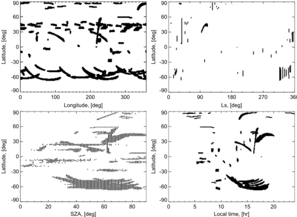
Figure 2. Coverage of OMEGA dayside limb spectra analyzed in this work. (top left) Latitude versus longitude; (top right)
latitude versus solar longitude (Ls) ; (bottom left) latitude versus SZA; (bottom right) latitude versus local time.
#171, #1343, #2295, #3400, #4500, #5600, #6690, #7650, #8810, #9700, and #10900. For this study, we have performed a manual verification of the sign of the shift for all our limb observations due to the uncertainty of the direction of the observation. The geocube information of our limbs’ LWIR data is now accurate to within the nearest pixel.
2.3. OMEGA Limb Observations
OMEGA works usually in nadir pointing to map the surface of Mars, but part of its operation time is also dedi-cated to probe the Martian atmosphere in limb viewing. For this study we used 98 dayside limb cubes acquired during the limb scans starting from the beginning of the mission in January 2004 up to orbit 7718 acquired in
Figure 3. OMEGA limb images at wavelengths of 2.30μm, 4.26μm, and 4.30μm from the cube 1619_4. The x dimension for this cube is 64 pixels. The 4.26μm and 4.30μm images are shifted in the y axis with regard to the 2.30μm image to account for the geometric correction.
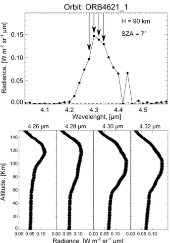
Figure 4. (top) OMEGA spectrum from orbit 4621_1 corresponding to a tangent altitude of 90 km and a SZA of7∘. The dashed line represents the radiometric offset. Arrows mark the wavelengths selected for the bottom panel. (bottom) Vertical profiles of OMEGA radiances at 4.26, 4.28, 4.30, and 4.32μm formed by combining all pixels from this cube.
January 2010 (Martian years ∼27–29). We have removed observations that were measured with a nonnomi-nal detector temperature and those whose OBC (On Board Calibration of the LWIR channel at the beginning of every orbit) was not correct (<335 digital units). In addition, we restricted our study to data with a solar zenith angle (SZA)< 90∘ (dayside). The coverage of OMEGA limb observations used for this study as function of longitude, latitude, solar longitude, SZA, and local time is shown in Figure 2. As can be seen from Figure 2 (top left), each OMEGA cube can cover several longitudes and latitudes. The data selected for this study present a very good latitudinal coverage of both hemispheres and they are spanning over more than 3 Martian years.
An example of OMEGA limb 2-D image at three different wavelengths is given in Figure 3. At 2.30 μm, only the surface of the planet and the atmospheric aerosols are visible. This wavelength has been used for sur-face/mineralogy mapping on Mars extensively in the past, including IRS/Mariner 6 and 7 and ISM/Phobos 2 [Erard and Calvin, 1997]. The strong non-LTE emission of the Martian atmosphere becomes clearly visible above the limb at a tangent altitude of about ∼90 km at 4.26 μm and 4.30 μm. These emissions do not show up clearly in nadir observations since their relative contribution is much smaller in nadir geometry [López-Valverde et al., 2005; Peralta et al., 2015]. Each pixel of Figure 3 is associated to one individual spectrum. Figure 4 (top) displays a typical OMEGA spectrum (from one single pixel) taken at the limb in the 4.3 μm region corresponding to a tangent altitude of 87 km and a SZA of 60∘. The spectrum was extracted from orbit 4621_1 at a latitude of∼−16∘. The intensity of the signal is well above the noise level in the wavelength range 4.20–4.50 μm and it exhibits a strong emission at 4.30 μm identified as CO2fluorescence
[Drossart et al., 2006], a non-LTE situation where the emission varies strongly with altitude and with SZA. At wavelengths smaller and greater than 4.30 μm, the intensity of the fluorescence decreases. At about 4.42 μm (spectel 220) there is a bad data value, present in the whole OMEGA data set (spectels 220–222).
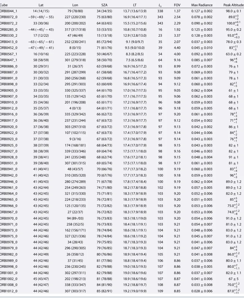
Table 1. List of the Cubes Analyzed in This Worka
Cube Lat Lon SZA LT Ls FOV Max Radiance Peak Altitude
ORB0044_1 14(14∕15) 79 (78/80) 34 (34/35) 13.7 (13.6/13.9) 338 1.37 0.127 ± 0.002 98.0 ± 0.1 ORB0072_0 −59 (−69∕ − 55) 227 (220/230) 75 (63/80) 16.9 (16.4/17.1) 343 2.54 0.078 ± 0.002 89.0+3 −2 ORB0072_2 33 (30/36) 200 (200/202) 64 (63/65) 15.5 (15.2/15.6) 343 2.29 0.090 ± 0.002 100.0+0−4.1 ORB0285_0 −44 (−45∕ − 43) 317 (317/318) 53 (53/55) 10.8 (10.7/10.8) 16 1.92 0.125 ± 0.003 95.0 ± 0.2 ORB0330_2 17 (12/22) 47 (46/49) 15 (13/18) 12.9 (12.8/13.0) 23 3.37 0.128 ± 0.003 93.0+4−0.3 ORB0413_0 −63 (−65∕ − 61) 232 (230/241) 85 (72/94) 9.1 (9.0/9.7) 35 2.07 0.037 ± 0.003 78.0 ± 0.3 ORB0452_0 −47 (−49∕ − 41) 8 (0/15) 71 (61/76) 9.5 (9.0/10.0) 39 4.40 0.045 ± 0.010 83+11 −3 ORB0567_1 16 (10/16) 225 (223/228) 50 (46/67) 8.3 (8.2/8.5) 54 4.00 0.092 ± 0.003 63.0 ± 0.2 ORB0647_1 58 (58/59) 301 (279/318) 58 (50/70) 7.5 (6.5/8.6) 64 9.16 0.085 ± 0.007 96+4 −6 ORB0886_0 30 (29/31) 31 (26/37) 63 (59/68) 16.9 (16.5/17.2) 93 8.99 0.072 ± 0.003 76 ± 1 ORB0887_0 30 (30/32) 291 (287/299) 61 (58/68) 16.7 (16.4/17.2) 93 9.08 0.069 ± 0.003 79 ± 1 ORB0891_0 31 (30/33) 260 (256/268) 62 (59/68) 16.8 (16.5/17.3) 93 9.09 0.061 ± 0.003 78 ± 1 ORB0898_0 33 (32/34) 295 (291/303) 63 (60/69) 16.9 (16.6/17.4) 94 9.12 0.060 ± 0.003 82+1 −5 ORB0905_0 33 (33/35) 330 (325/337) 64 (61/70) 17.0 (16.7/17.5) 95 9.05 0.062 ± 0.004 61 ± 1 ORB0907_0 34 (33/35) 135 (129/142) 65 (61/70) 17.1 (16.7/17.5) 95 9.06 0.062 ± 0.003 68 ± 1 ORB0910_0 35 (34/36) 201 (196/208) 65 (61/71) 17.2 (16.9/17.7) 96 9.08 0.059 ± 0.003 68 ± 1 ORB0912_0 35 (35/37) 4 (0/13) 64 (61/71) 17.1 (16.8/17.7) 96 9.18 0.059 ± 0.005 68 ± 1 ORB0916_0 36 (36/39) 335 (329/342) 66 (62/72) 17.3 (16.9/17.7) 97 9.20 0.061 ± 0.003 78+1−3 ORB0917_0 36 (36/40) 237 (231/244) 67 (63/72) 17.3 (16.9/17.7) 97 9.12 0.054 ± 0.002 71+4 −1 ORB0920_0 37 (36/38) 303 (297/310) 67 (63/72) 17.3 (16.9/17.8) 97 9.13 0.042 ± 0.002 86 ± 1 ORB0922_0 37 (37/38) 107 (102/115) 67 (63/73) 17.4 (17.0/17.9) 97 9.14 0.044 ± 0.006 84+1 −2 ORB0923_0 37 (37/38) 9 (3/16) 67 (63/72) 17.3 (16.9/17.8) 97 9.14 0.043 ± 0.003 76+4−1 ORB0925_0 38 (37/39) 174 (168/181) 68 (64/73) 17.4 (17.0/17.9) 98 9.15 0.043 ± 0.003 82 ± 1 ORB0927_0 38 (38/39) 339 (333/346) 69 (64/74) 17.5 (17.1/18.0) 98 9.16 0.046 ± 0.003 82 ± 1 ORB0928_0 39 (38/41) 241 (235/248) 68 (62/74) 17.6 (17.2/18.1) 98 9.15 0.048 ± 0.004 91 ± 1 ORB0931_0 39 (38/40) 307 (301/315) 69 (65/74) 17.5 (17.1/18.0) 98 9.17 0.061 ± 0.003 81 ± 1 ORB0941_0 41 (40/41) 48 (43/57) 70 (66/76) 17.7 (17.3/18.2) 100 9.19 0.060 ± 0.003 83+1−4 ORB0942_0 41 (40/42) 310 (305/320) 70 (67/76) 17.7 (17.3/18.3) 100 9.18 0.059 ± 0.003 96+1−3 ORB0946_0 41 (40/43) 280 (274/289) 71 (67/78) 17.8 (17.4/18.4) 100 9.19 0.062 ± 0.004 89.0 ± 1.2 ORB0961_0 43 (42/44) 254 (249/263) 74 (71/80) 18.2 (17.8/18.8) 102 9.19 0.057 ± 0.005 89.0 ± 1.2 ORB0964_0 43 (42/45) 321 (315/330) 75 (71/81) 18.3 (17.9/18.9) 103 9.20 0.052 ± 0.006 82.0 ± 1.2 ORB0965_0 43 (42/45) 224 (218/233) 76 (72/81) 18.3 (17.9/18.9) 103 9.20 0.051 ± 0.005 85+5−4 ORB0966_0 43 (42/45) 125 (120/135) 75 (72/82) 18.3 (17.9/18.9) 103 9.20 0.053 ± 0.006 75.0+1.2 −7 ORB0967_0 43 (42/45) 27 (22/37) 76 (72/82) 18.3 (17.9/18.9) 103 9.20 0.053 ± 0.006 74.0+1−8.2 ORB0970_0 44 (42/45) 94 (89-/03) 76 (73/83) 18.5 (18.1/19.0) 103 9.20 0.054 ± 0.006 91.0 ± 1.2 ORB0971_0 44 (42/45) 258 (352/5) 76 (73/83) 18.4 (18.1/19.1) 103 9.21 0.054 ± 0.007 81.0 ± 1.2 ORB0973_0 44 (42/46) 162 (156/171) 78 (74/84) 18.6 (18.1/19.1) 104 9.21 0.048 ± 0.006 83.0 ± 1.2 ORB0975_0 44 (42/46) 327 (321/336) 78 (74/84) 18.6 (18.1/19.2) 104 9.21 0.045 ± 0.007 91.0 ± 1.2 ORB0978_0 44 (42/46) 34 (28/43) 79 (75/85) 18.7 (18.3/19.3) 104 9.21 0.041 ± 0.006 83.0 ± 1.2 ORB0979_0 44 (42/46) 296 (290/305) 79 (76/85) 18.7 (18.3/19.3) 104 9.21 0.047 ± 0.007 84+3 −4 ORB0982_0 44 (42/49) 26 (358/12) 80 (76/86) 18.9 (18.4/19.4) 105 9.21 0.041 ± 0.008 86.0+1−2.2 ORB0989_0 44 (42/46) 37 (31/45) 81 (77/86) 18.8 (18.4/19.4) 106 8.86 0.037 ± 0.006 80.0 ± 1.1 ORB0998_0 44 (42/46) 236 (230/245) 82 (79/88) 19.0 (18.5/19.5) 107 8.86 0.038 ± 0.005 80.0+7−1.1 ORB1001_0 44 (42/46) 302 (297/311) 82 (79/88) 19.0 (18.6/19.6) 107 8.86 0.037 ± 0.007 82.0 ± 1.1 ORB1002_0 45 (43/47) 202 (198/213) 81 (78/88) 18.9 (18.6/19.6) 107 8.87 0.041 ± 0.006 67 ± 5 ORB1008_0 44 (42/47) 338 (333/347) 84 (81/90) 19.2 (18.8/19.7) 108 8.87 0.033 ± 0.008 70.0+1−5.2 ORB1012_0 44 (42/46) 307 (303/317) 85 (82/91) 19.2 (19.0/19.9) 109 8.85 0.028 ± 0.006 87.0+1.2 −11
Table 1. (continued)
Cube Lat Lon SZA LT Ls FOV Max Radiance Peak Altitude
ORB1023_0 4 (41/46) 313 (309/322) 89 (86/94) 19.6 (19.3/20.2) 110 8.86 0.018 ± 0.009 84.0 ± 1.2 ORB1084_0 79 (79/80) 207 (198/217) 72 (71/74) 4.1 (3.5/4.7) 118 3.09 0.069 ± 0.001 85 ± 1 ORB1402_0 86 (86) 348 (348/351) 82 (82) 5.9 (5.9/6.1) 162 1.59 0.055 ± 0.002 81.0+4.0 −0.1 ORB1619_4 −51 (−52∕ − 51) 323 (317/329) 60 (57/63) 8.6 (8.2/9.0) 196 6.50 0.111 ± 0.003 99.0+0.5 −1 ORB2505_3 16 (10/16) 227 (225/229) 41 (26/61) 9.6 (9.4/9.7) 345 3.35 0.113 ± 0.003 69.0+3−0.0.2 ORB2547_2 27 (26/28) 49 (46/53) 59 (57/62) 8.4 (8.2/8.6) 352 4.20 0.089 ± 0.002 85.0+4.0 −0.2 ORB2648_0 47 (47/48) 220 (218/223) 61 (60/63) 8.6 (8.4/8.7) 6 6.35 0.091 ± 0.003 85.0 ± 0.1 ORB2958_0 30 (27/31) 143 (143/144) 30 (29/31) 14.3 (14.3/14.4) 46 8.79 0.076 ± 0.003 105.0 ± 1.1 ORB2996_0 46 (46/50) 51 (47/62) 58 (56/66) 16.2 (16.0/17.0) 51 9.59 0.053 ± 0.002 72+21−10 ORB3024_0 49 (48/53) 180 (174/188) 56 (52/61) 16.0 (15.6/16.6) 54 9.18 0.058 ± 0.001 83+15−14 ORB3769_2 −9 (−11∕ − 6) 2 (359/5) 66 (63/69) 7.7 (7.5/7.9) 150 5.24 0.062 ± 0.001 98+2 −6 ORB4062_2 0 (0) 217 (217/218) 84 (84/85) 17.6 (17.6/17.7) 195 2.06 0.025 ± 0.002 92.0 ± 0.2 ORB4483_1 −4 (−10∕ − 2) 259 (254/261) 25 (4/52) 13.1 (12.8/13.2) 268 2.37 0.153 ± 0.003 107.0+2 −0.1 ORB4621_1 −16 (−19∕ − 12) 25 (20/28) 6 (0/17) 11.7 (11.3/11.8) 292 2.91 0.151 ± 0.001 104.0 ± 0.1 ORB4706_3 −9 (−12∕ − 7) 309 (304/312) 22 (19/28) 10.5 (10.1/10.7) 306 3.65 0.140 ± 0.003 96+0.2 −3 ORB4768_0 −44 (−59∕ − 40) 18 (14/43) 29 (23/48) 12.4 (12.1/14.1) 316 3.85 0.135 ± 0.003 103 ± 0.2 ORB4768_0 −64 (−66∕ − 59) 93 (43/104) 70 (49/74) 17.5 (14.1/18.1) 316 2.00 0.075 ± 0.005 91+2 −0.2 ORB4781_0 −45 (−63∕ − 41) 182 (178/223) 30 (25/52) 12.4 (12.1/15.1) 318 3.85 0.132 ± 0.003 102+1 −0.2 ORB4781_0 −63 (−65∕ − 57) 259 (200/279) 71 (53/80) 17.6 (13.6/18.9) 318 2.01 0.074 ± 0.005 86.0 ± 0.3 ORB4787_0 −50 (−64∕ − 45) 317 (311/3) 35 (30/54) 12.6 (12.2/15.7) 319 3.50 0.129 ± 0.003 101.0 ± 0.2 ORB4787_0 −59 (−64∕ − 57) 39 (337/54) 75 (55/79) 18.1 (13.9/18.6) 319 1.79 0.064 ± 0.003 88.0 ± 0.3 ORB4810_0 2 (1/4) 166 (162/168) 44 (42/48) 9.0 (8.7/9.1) 323 5.09 0.114 ± 0.004 98.0 ± 0.1 ORB4822_0 −45 (−62∕ − 40) 117 (113/159) 31 (26/50) 12.3 (12.0/15.0) 325 4.16 0.127 ± 0.003 98.0 ± 0.2 ORB4822_0 −59 (62∕ − 55) 191 (133/202) 70 (51/75) 17.1 (13.2/17.9) 325 2.24 0.072 ± 0.003 87.0+0−2.3 ORB4858_0 −47 (−59∕ − 43) 186 (180/233) 36 (31/55) 12.3 (11.8/15.4) 330 4.14 0.122 ± 0.003 96 ± 0.2 ORB4858_0 −54 (−59∕ − 49) 258 (208/275) 71 (56/80) 7.1 (13.7/18.2) 330 2.25 0.071 ± 0.003 83.0 ± 0.3 ORB4890_0 −48 (−57∕ − 46) 288 (281/333) 39 (35/56) 12.3 (11.8/15.3) 335 4.14 0.117 ± 0.002 92.0 ± 0.2 ORB4890_0 −50(−57∕ − 46) 238 (328/11) 71 (57/78) 17.0 (14.9/17.7) 335 2.23 0.066 ± 0.002 87.0 ± 0.3 ORB4931_0 −44(−54∕ − 41) 218 (211/263) 37 (34/51) 11.9 (11.4/14.8) 341 4.79 0.117 ± 0.003 97.0+1 −0.2 ORB4931_0 −49(−54∕ − 46) 282 (239/290) 65 (52/69) 16.1 (13.2/16.6) 341 2.83 0.075 ± 0.003 79.0+1−0.2 ORB4956_0 −41(−49∕ − 38) 280 (274/302) 35 (29/46) 11.5 (11.1/13.0) 345 5.36 0.112 ± 0.004 91.0+1−0.2 ORB4956_0 −49(−50∕ − 47) 338 (297/347) 60 (47/64) 15.4 (12.6/16.0) 345 3.36 0.083 ± 0.003 86.0 ± 0.2 ORB4973_0 −39(−48∕ − 36) 48 (43/81) 34 (33/47) 11.4 (11.0/13.5) 348 5.71 0.116 ± 0.003 109.0 ± 0.3 ORB4973_0 −48(−49∕ − 46) 106 (81/115) 58 (48/62) 15.2 (13.5/15.8) 348 3.61 0.083 ± 0.003 81.0 ± 0.4 ORB5006_0 27 (21/29) 86 (80/107) 33 (32/43) 13.1 (12.6/14.4) 352 6.19 0.117 ± 0.002 92 ± 1 ORB5006_0 16 (14/22) 118 (106/121) 52 (44/55) 15.2 (14.4/15.4) 352 4.24 0.095 ± 0.002 81 ± 1 ORB5023_0 28 (23/30) 206 (201/228) 33 (16/37) 13.0 (12.5/14.3) 355 5.91 0.120 ± 0.003 94+2 −1 ORB5023_0 17 (11/26) 239 (219/248) 50 (38/59) 15.1 (13.7/15.7) 355 4.03 0.098 ± 0.003 75 ± 2 ORB5330_0 18 (7/49) 219 (218/225) 62 (62/64) 16.3 (16.1/16.6) 36 1.94 0.072 ± 0.004 78 ± 1 ORB5330_0 50 (41/56) 226 (224/229) 65 (65/67) 16.7 (16.6/16.9) 36 1.68 0.073 ± 0.003 92.0+2−0.2 ORB5851_0 −29 (−29∕ − 25) 256 (252/260) 64 (50/81) 9.2 (9.0/9.5) 102 6.81 0.073 ± 0.004 79.0+0.1 −1 ORB6071_1 86 (85/88) 85 (70/95) 74 (73/76) 23.4 (23.9/0.0) 131 2.76 0.065 ± 0.004 92.0 ± 2 ORB6104_1 80 (80/81) 116 (107/129) 74 (72/76) 5.3 (4.7/6.1) 136 3.29 0.069 ± 0.003 97.0 ± 1 ORB6126_1 76 (76/77) 80 (72/89) 75 (73/77) 5.5 (4.9/6.0) 139 3.59 0.067 ± 0.002 80 ± 1 ORB6146_0 78 (78/79) 88 (80/96) 78 (76/80) 19.1 (18.5/19.6) 142 2.88 0.059 ± 0.003 86.0+0.1 −4 ORB6586_0 −53 (−58∕ − 47) 238 (230/244) 53 (45/58) 14.8 (14.3/15.2) 211 3.35 0.134 ± 0.003 100+1−3 ORB7554_4 −59 (−61∕ − 56) 343 (353/0) 67 (63/70) 13.5 (13.3/13.7) 13 4.75 0.085 ± 0.003 96.0+5−0.3
Table 1. (continued)
Cube Lat Lon SZA LT Ls FOV Max Radiance Peak Altitude
ORB7586_4 −53 (−56∕ − 50) 8 (6/11) 63 (58/73) 13.1 (13.0/13.3) 17 4.75 0.086 ± 0.003 85+2−4 ORB7597_4 −51 (−54∕ − 49) 338 (337/341) 61 (58/64) 13.0 (12.9/13.1) 19 4.75 0.089 ± 0.003 97+3 −1 ORB7604_4 −50 (−53∕ − 47) 352 (351/355) 60 (55/63) 12.9 (12.8/13.1) 20 4.75 0.094 ± 0.002 82 ± 3 ORB7619_4 −48 (−50∕ − 44) 279 (279/281) 58 (51/61) 12.7 (12.7/12.8) 22 4.75 0.096 ± 0.001 99+2 −3 ORB7679_0 86 (86/87) 286 (285/291) 76 (76) 7.7 (7.6/8.0) 30 2.20 0.066 ± 0.002 83.0+0−1.2 ORB7686_0 86 (86/87) 277 (277/282) 77 (76/77) 6.1 (6.1/6.4) 31 2.19 0.065 ± 0.002 86.0+0.2 −2 ORB7694_0 86 (86/87) 168 (162/175) 77 (77/78) 4.6 (4.1/5.0) 32 2.21 0.063 ± 0.002 85.0 ± 0.2 ORB7697_0 86 (86/87) 223 (217/231) 77 (77/78) 4.4 (3.9/4.9) 32 2.22 0.062 ± 0.002 86.0 ± 0.2 ORB7701_0 85 (85/87) 165 (157/173) 78 (78/79) 3.3 (2.8/3.9) 33 2.21 0.060 ± 0.002 85.0 ± 0.2 ORB7708_0 86 (86/87) 192 (186/200) 77 (77) 4.2 (3.7/4.6) 34 2.32 0.062 ± 0.002 84.0 ± 0.2 ORB7715_0 86 (86/87) 212 (207/220) 76 (76/77) 4.5 (4.1/5.0) 34 2.40 0.061 ± 0.002 85.0+1−0.2 ORB7718_0 86 (86/87) 274 (268/281) 76 (76) 4.7 (4.3/5.2) 35 2.46 0.059 ± 0.002 83.0 ± 0.2
aIn the table are reported the average values of the latitude (deg), longitude (deg), solar zenith angle (deg), local time (h), solar longitude (deg), field of view
(km), maximum radiance±1𝜎(W m−2sr−1μm), and tangent altitude of the peak emission (km). Values in parentheses correspond to the intervals of latitudes,
longitudes, local times, and SZAs for each cube. Errors on the tangent altitude of the peak emission are also given; see text for details.
OMEGA observations allow to determine the tangent altitudes of the non-LTE emission at each wavelength. Notice that in the case of limb observations, the altitude of the pixel central point is replaced with the alti-tude of the central tangent point above the surface of Mars. Figure 4 (bottom) displays the vertical profiles of OMEGA radiances at four different wavelengths obtained with all the spectra of the 4621_1 cube. A peak in the emission is clearly observed at each wavelength, the altitude of the peak decreases with wavelength from about 120 km to 95 km.
2.4. Vertical Radiance Profiles at 4.30𝛍m
One of the quantities that has been analyzed in detail is the peak altitude of the non-LTE emission at 4.30 μm. This altitude depends on the structure of the whole atmosphere below and represents a strong validation tool for atmospheric models.
The OMEGA detector array is not always aligned with the limb horizon of Mars at the tangent point, and there-fore, building individual vertical profiles cannot be done simply from individual rows of pixels. For each cube, we averaged the radiances at every level of a fixed altitude grid in order to determine accurately the average tangent altitude of the peak of the non-LTE emission at 4.30 μm. The possible error sources on the determina-tion of the peak emission tangent altitude are (1) the pointing error and (2) the real variability in the radiance within each cube. The pointing error generally varies between few hundreds of meters and 1 km depending on the distance of the spacecraft from the planet. To estimate the second type of uncertainty for each cube we made a series of test creating synthetic vertical radiance profiles by superimposing a random value within the noise on the radiance. We then determined the peak emission altitude for all synthetic vertical profiles within each cube, and we assumed as error on the tangent altitude the minimum and maximum values obtained for each series of profiles. The error on the peak emission altitude ranges from 1 to 2 km up to ∼20 km in few spe-cial cases (see Table 1). Figure 5 (top) shows an example of vertical profile obtained by combining the radiance at 4.30 μm of all pixels from the cube 7619_4 together with the average profile (red line). At this wavelength the radiance reaches a maximum value of 0.09 W m−2sr−1μm at 99 km. Notice that the latitude, local time (LT),
solar zenith angle (SZA), and solar longitude (Ls) vary within each cube. In most cases, such variations are small for the solar zenith angle and the local time; therefore, extracting a representative average profile of the whole cube does make sense. However, for some cubes the geometry of observation allowed to scan the limb twice yielding two “profiles” with different SZA and LT. This is the case, for example, of cube 4768_0 (Figure 5, bottom). Since non-LTE radiances are strongly dependent on solar illumination conditions, as predicted by the non-LTE model [López-Valverde and López-Puertas, 1994a], radiances from cube 4768_0 can easily be split in two separate vertical profiles corresponding to an average SZA of 29∘ and 70∘. As the SZA increases, the peak intensity decreases from 0.13 W m−2sr−1μm at 103 km to 0.07 W m−2sr−1μm at 91 km. Notice that the
Figure 5. Vertical profiles obtained by combining the OMEGA radiance (black crosses) at 4.30μm of all the pixels from cubes (top) 7619_4 and (bottom) 4768_0. Cube 4768_0 presents two vertical profiles corresponding to an average SZA of 29∘and 70∘. Red lines represent the vertical average profiles used to determine the tangent altitudes at which the emissions reach their maximum.
The analyzed cubes are listed in Table 1, together with details on observation, such as the Lsand the field of
view (FOV). In addition, Table 1 contains for each cube the values of the maximum radiance at 4.30 μm, the tangent altitude where this maximum occurs (the peak emission) and the corresponding values of latitude, longitude, SZA, and LT.
3. Vertical Variation and Model Interpretation
The non-LTE model used for this study is described by López-Valverde and López-Puertas [1994a, 1994b]. This model has been tested and updated against a few PFS/MEx spectra for the Mars atmosphere [López-Valverde
et al., 2005, 2011; Gilli et al., 2011] and against a few CO2spectra from VIRTIS/VEx in Venus [López-Valverde
et al., 2007]. According to the model, and for a given reference atmosphere, two factors mostly affect the
non-LTE radiances: (1) the thermal structure (affecting the tangent altitude of the peak emission) and (2) the solar illumination conditions, or SZA, especially affecting the intensity of the emission. Therefore, we analyze the behavior of the emission as function of these two parameters and compare the observations to simulated non-LTE emissions.
Three reference atmospheres were used to perform the radiance simulations compared to the OMEGA data. They are shown in Figure 6 and correspond to a “cold” and a “warm” atmospheric state, in addition to a profile extracted from the LMD Mars GCM simulation obtained for the conditions of the OMEGA cube 1619_4. We used the peak altitude of the non-LTE emission at 4.30 μm as key parameter to compare the model to the data. As first approximation, this altitude is linked to a well-defined pressure layer. With the main goal to determine this pressure level, we therefore performed non-LTE simulations for 16 different input atmospheres that
Figure 6. Vertical profiles of the atmospheric thermal structure used in the simulations, extracted from the LMD Mars
GCM, version 5, as a function of (left) altitude and (right) pressure. The profile labeled 1619 corresponds to a location and season close to the OMEGA cube ORB1619_4, specifically latitude = 51∘S, longitude = 37∘W, SZA = 60∘, andLs= 9∘. The location of the peak emission at 4.30μm is also shown.
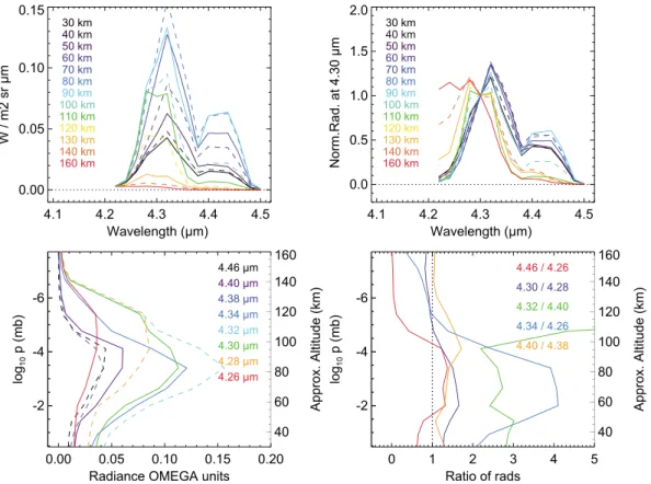
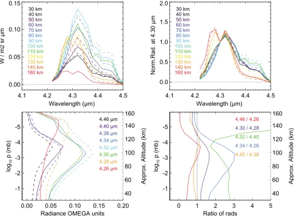
Figure 7. Non-LTE model simulations of the CO2spectra in the 4.3μm region for the cold reference atmosphere. (top left) Averaged spectra in 10 km boxes at 13 different altitudes. (top right) The 13 spectra but normalized at the 4.3μm value at each tangent altitude. (bottom left) Variation with tangent altitude of eight individual wavelengths. (bottom right) Vertical profiles of five different ratios between pairs of wavelengths, as indicated. See text.
Figure 8. Same as Figure 7 but for the warm model atmosphere. See text.
represent extreme cases and include the cold and warm scenarios mentioned above. We derived an average value for the pressure level of the peak emission that corresponds to 0.03 ± 0.01 Pa. If SZA is varied between 0∘ and 80∘, an additional 0.01 Pa variation around the 0.03 Pa is obtained. We will use this reference pressure level throughout this work.
3.1. Vertical Variation
Figure 7 presents simulations obtained with the non-LTE model and a line-by-line radiative transfer code of the CO2limb emission in the 4.3 μm region at 13 different tangent altitudes, from 30 to 160 km, using the cold
reference atmosphere of Figure 6. This reference atmosphere is a standard thermal structure with a tropo-sphere near convective equilibrium, a relatively cold mesotropo-sphere, and a surface temperature and pressure of 214 K and 6.7 mbar, respectively (Figure 6). The simulations were performed at high spectral resolution, then degraded to a 14 cm−1resolution, and then sampled at the OMEGA wavelength points. Figures 7 (top left) and
7 (bottom left) show what we consider is a typical variation with tangent altitude, with a signal increasing with tangent altitude at all wavelengths from 30 to about 80–90 km, peaking around 80 km, and then decreas-ing with tangent altitude. The decrease with tangent altitude is particularly significant in the 4.38–4.50 μm region, whose emission decreases below OMEGA noise levels above about 110 km. However, the emission between 4.24 and 4.34 μm is still significant at 130 km. The specific CO2rovibrational bands that contribute
to the emission are the same than those identified by López-Valverde et al. [2005] in their study of PFS and infrared space observatory (ISO) nadir observations. The 4.38–4.50 μm region is dominated by the second hot bands of the 636 isotope, while the strongest emission around 4.30 μm contains contributions from many bands, dominated by the second hot bands of the main isotope and diverse bands from the 2.0 μm system (direct solar pumping around 2.0 μm and radiative cascading to lower states).
The shape of the 4.3 μm spectra changes with tangent altitude, as shown in Figure 7 (top right), where the spectra are normalized to the 4.30 μm value. We see that from 30 to about 90 km the spectral shape does not change significantly, which indicates that the major contributing bands are near saturation at tangent alti-tude below the peak. Above the peak, the isotopic 636 bands (4.40–4.44 μm) are optically thin and decrease strongly with tangent altitude, following the exponential decrease in density, but the second hot bands of the main isotope 626 are still optically thick. They dominate the limb emission between 100 and 130 km,
Figure 9. Same as Figure 7 but using the reference profile 1619 from Figure 6. These results should be compared to the
measurements in Figure 10. See text for details.
with a double peak structure at 4.28 and 4.32 μm, where the lines of the P and R branches of these bands are strongest. This double peak is clearer in Figure 8. Higher up, the 626 fundamental band is the only important contribution and a double peak with a central dip at 4.25 μm appears at 160 km, which is the center of this band. A similar behavior is observed in the Venus atmosphere [Gilli et al., 2009].
The vertical profiles at eight different wavelengths are shown in Figure 7 (bottom left). Figure 7 (bottom right) shows diverse radiance ratios between several pairs of wavelengths. These variations with tangent altitude should be compared to the OMEGA data and may represent a strong test for the non-LTE model.
The peak of the whole 4.3 μm emission occurs around 0.03 ± 0.01 Pa, which corresponds to 85 km for this particular Mars atmosphere. This altitude is very dependent on the thermal structure (scale heights) below the peak. The pressure level of the peak emission, however, is highly independent on the actual thermal structure. This is because this CO2emission corresponds to a fluorescent mechanism, dictated by the solar flux and its
penetration into the atmosphere, i.e., its primary factor is the column density of CO2above the peak. To illustrate the impact of the thermal structure, Figure 8 shows the results for a very different model atmo-sphere, the warm reference atmosphere; it has a similar tropoatmo-sphere, surface temperature, and pressure, but it is ∼50 K warmer above ∼60 km, i.e., much denser and warmer in the whole mesosphere (Figure 6). The characteristics of the altitude variation in the two regions, 4.24–4.34 and 4.38–4.50 μm, are similar but two major differences appear (see Figures 7–9). The first is that the peak altitudes in the warm model are about 20 km higher than in cold model, although the emission pressure is basically the same, in consonance with the warmer atmosphere. The second is the absence of the spectral dip at 4.38 μm, i.e., it does not show a clear separation between the isotopic components. The absence of the dip for the warmer atmosphere might be due to the larger 636 isotopic bands emission for this case. This is, however, not conclusive, because our model systematically underestimates the 636 isotopic components (see below).
Figure 9 shows the simulations for cube ORB1619_4. The reference atmosphere “1619” is almost an interme-diate case between the cold and warm scenarios (Figure 6). The spectral dip at 4.38 μm is present, but it is less
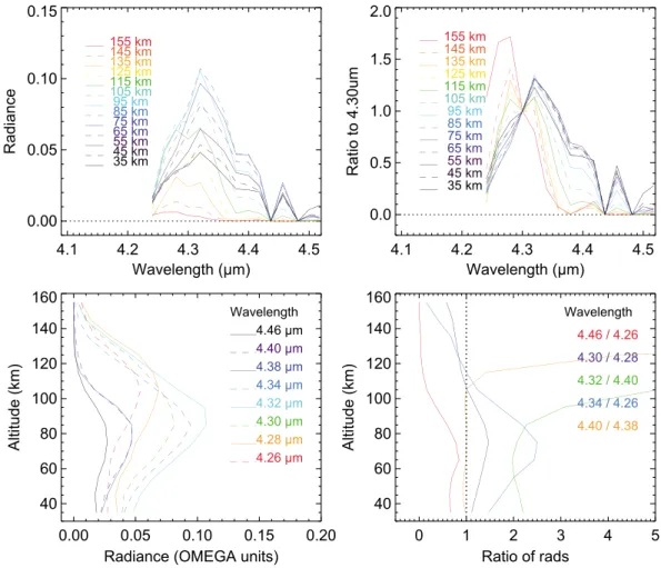
Figure 10. Same as Figure 7 but with OMEGA data from orbit 1619_4 (see text).
strong than in the cold scenario (Figure 7). Similarly, the double peak structure at 4.28 and 4.32 μm is less clear than in Figure 8.
Figure 10 shows the tangent altitude variation of OMEGA radiance observations from one particular orbit (ORB1619_4; Date = 21 April 2005, Lat = −51∘, Long = 323∘, SZA = 60∘), after averaging the data in 10 km boxes to reduce noise to some degree. The measurements have been corrected by subtracting the radiation offset and 1-point spectral shift was applied. This figure can be directly compared to Figures 7–9. The major features and characteristics of the observations are reproduced by the model. In particular, the increase in the intensity of the whole 4.3 μm emission with tangent altitude up to some height in the mesosphere (in this example/orbit the peak is around 72 km) and a fast decrease above the peak. The spectral shape of the whole band is also changing with tangent altitude in good agreement with the model: it presents a maximum at 4.32 μm up to about a few scale heights above the peak of whole band at ∼85 km (Figure 10, top right). Above this point, starting from 95 km, spectra show the double peak at 4.28 and 4.32 μm. One difference (see Figure 9) is the bump around 130 km in the simulations which is absent in the measurements, especially prominent in the 4.28 and 4.32 μm wavelengths, i.e., in the second hot bands of the CO2major isotope. Perhaps the main difference between data and model is the relative magnitude of the emission in the 4.38–4.48 μm region, larger in the data than in the model at mesospheric altitudes. Even the simulation for the warm atmosphere used in Figure 8 produces a slightly lower emission. The more realistic atmospheric structures used in Figure 7 and 9 show, in addition, the dip at 4.38 μm which is not observed in the data. Perhaps some CO2band or set of weak bands are missing in the model [López-Puertas et al., 1998].
Let us recall that these simulations, especially the one in Figure 9, combine results from the GCM and from the non-LTE model, and it is difficult to draw conclusions about only one of them from a comparison like this. However, systematic studies like this but extended to the whole data set and comparisons to many warm and
Figure 11. Study of the variation with SZA in OMEGA observations. (top) Spectra for different SZA values at a fixed
tangent altitude (∼80 km) from different orbits and cubes, as indicated. (bottom) Cross section in tangent altitude and SZA of the 4.30μm emission from OMEGA orbit 647, cube 1.
cold cases are needed to determine biases in the models. The final goal, beyond the scope of this paper, will be the retrievals of the density and the thermal structure from these spectra.
3.2. SZA Variation
Figure 11 compares several individual spectra acquired from different orbits and cubes at a tangent altitude of 80 km and with a latitude ranging from −16∘ to 31∘ in order to study their dependence on SZA. As expected, the solar illumination plays an important role in the non-LTE excitation. The SZA in Figure 11 (top) varies from 7∘to 84∘ producing a decrease in the non-LTE emission. The decrease is not homogeneous because mixing different orbits includes atmospheric variability that changes the emission altitude. The decrease with SZA is clearer in Figure 11 (bottom), which only combines data from one data cube and orbit.
Figure 12 shows a similar study but with results from the model simulations for the cold reference atmosphere. In this case, the same model atmosphere is used for all the SZA calculations. Notice that the particular thermal structure affects important aspects like the altitude and the radiance of the peak emission, respectively, at ∼80 km and about 0.13 W m−2sr−1μm−1, for SZA = 60∘ in this case. Figure 12 (top) shows spectra at four
Figure 12. Study of the SZA effect on the model simulations for the cold model, to be compared to Figure 11.
(top) Spectra at SZA = 0, 60, 80, and 88∘for two tangent altitudes, 80 and 110 km, as indicated. (bottom) Cross section versus tangent altitude and SZA of the 4.30μm emission; same units as in Figure 11 (see text).
Figure 13. Tangent altitude of peak emission in OMEGA observations at 4.30μm in terms of solar zenith angle (SZA). The color scale indicates the intensity of the emission at 4.30μm.
Figure 14. Tangent altitude of the peak emission in OMEGA observations (black dots) at 4.30μm as function of Solar Longitude (Ls) compared to the altitude of constant pressure levels derived from SPICAM stellar occultations (blue dots). Panels correspond to different SPICAM pressure levels as follow: (top) pressure level = 0.01 Pa; (middle) pressure level = 0.02 Pa; and (bottom) pressure level = 0.03 Pa.
different SZAs and at two tangent altitudes, near the mesospheric peak and above the peak emission. The shape in the second case does not change with SZA, while in the first case there is a slight modification in the spectral shape: at higher SZA (lower solar illumination) the 636 isotopic emission is a little less prominent and the dip at 4.38 μm tends to disappear. This variation is difficult to be confirmed with OMEGA since the extraction of a pure SZA variation from one orbit is not possible. Figure 12 (bottom) shows a general pattern of a decrease of the radiance toward higher SZA, specially rapid at the peak emission altitude, and this is observed in both data and model. Another interesting prediction of the non-LTE model at the 4.30 μm spectel is that the decrease of radiance with SZA is slower around 115 km, i.e., a few scale heights above the peak altitude. This tends to create a vertical profile with a double peak: a main peak around 80 km and a secondary peak around 120 km.
Figure 13 shows the variation of the tangent altitude and magnitude of the peak emission with SZA observed by OMEGA at 4.30 μm. The data correspond to the values in Table 1 and again, contain a large spatial and temporal variability. The clear trend in the peak altitude observed in the data is absent in the non-LTE
simulations in Figure 12 when using a fixed atmospheric profile. However, we expect the OMEGA data to show a variation larger than that in the non-LTE model for two reasons. First, because of possible uncertain-ties in the non-LTE model and its evaluation of the SZA variation, although we believe this to be a small effect. Second, because there are atmospheric changes associated to the SZA and the local time which are not included in the simulations in Figure 12. This is what is found in Figure 13. The trend observed may partially contain a SZA intrinsic effect and mostly an atmospheric variability due to local time effects. In addition to this trend, Figure 13 shows, at each SZA value, a clear variability that cannot be explained in terms of non-LTE alone but must be associated to changes in the atmospheric thermal state in space and time. In the next sections we will analyze this latter variability in more detail.
4. Comparison to SPICAM/Mars Express Stellar Occultations
The ultraviolet spectrometer SPICAM on board Mars Express measures density and temperatures profiles of the upper atmosphere of Mars (between 60 and 130 km) using the stellar occultation technique. One Martian year of observations (MY27), from 14 January 2004 to 11 April 2006, was analyzed by Forget et al. [2009]. Figure 14 compares the altitude of OMEGA peak emission with the altitudes of the 0.01 (top), 0.02 (middle), and 0.03 Pa (bottom) levels derived from SPICAM stellar occultations. For this figure 468 SPICAM stel-lar occultations were used, all acquired on the nightside for latitudes in between −50∘ and 50∘. The uncertainty in the altitude of the pressure levels as deduced from the SPICAM observations primarily result from the uncer-tainty on the CO2densities and temperatures. At the pressure levels used here, the point to point uncertainties
are estimated to be around 10% [see Forget et al., 2009], which convert in less than 1.5 km here assuming a scale height of 7 km. The absolute altitude may also be affected by a systematic bias due to uncertainties in the CO2spectroscopy, up to 2 km. As can be seen in Figure 14, a better agreement seems to occur at 0.01 Pa;
however, direct comparison between the two data set is not easy since SPICAM measurements are acquired on the nightside, unlike the OMEGA data. The atmospheric pressures observed by SPICAM mainly vary with seasons. The altitude of a constant pressure level is minimum around the southern winter solstice (Ls= 90∘)
and maximum around the Mars perihelion (Ls = 251∘). The altitude of OMEGA peak emission shows a
simi-lar seasonal variability, with a minimum around the Mars aphelion and maximum in the perihelion. However, the peak emission altitudes from OMEGA are more scattered than the pressure level altitudes retrieved from SPICAM, especially near the southern winter solstice (Ls∼ 100∘). Most of the OMEGA data for this Lscorrespond to the same Martian year (MY27), to high SZA (61–89∘) and similar latitude (30–45∘) (See Table 1). The compar-ison to SPICAM observations illustrates very well that the OMEGA peak emission altitude is indeed correlated with the variation of pressure level altitudes; however, since SPICAM stellar occultations are performed dur-ing nighttime, we cannot conclude which pressure level exactly correlates the best with the emission durdur-ing daytime.
5. Comparison With a GCM Model
According to the non-LTE simulations presented above, the tangent altitude of the limb peak emission varies with the atmospheric conditions but the pressure of the layer is approximately fixed at about 0.03 ± 0.01 Pa. Therefore, the altitude variability of the peak emission should be closely tied to the altitude variations produced by the atmospheric expansion and contraction.
In this section we compare the OMEGA observed peak altitudes with the altitude of the 0.03 Pa pressure level predicted by a Mars global climate model (MGCM) in its latest version extending from the surface to the exobase [González-Galindo et al., 2013, 2015]. This version takes into account the observed day-to-day variability of the UV solar flux and of the lower atmospheric dust load for Martian years 24 to 31. For each OMEGA observation, corresponding to Martian years 26 to 30, we have extracted from the corresponding MGCM simulation the altitude of the 0.03 Pa isobar at the time, location, and SZA of the observations and compared to the observed value. To evaluate the variability predicted by the model, we extracted also the altitude of the isobar in a range of ±5∘ in latitude and longitude and Ls, and ±0.5 local hours.
Figure 15 (top) displays the latitude-local time variation of the peak emission altitude at 4.30 μm using OMEGA observations. For comparison, Figure 15 (bottom) shows the same plot obtained from the GCM. Both the model and the data show the highest altitudes around noon, consistent with the expected higher tempera-tures in the lower atmosphere. However, the range of measured tangent altitudes (between 61 and 109 km) is clearly much larger than the MGCM predicted altitude variability (76 to 91 km).
Figure 15. (top) Variation in the OMEGA data of the altitude of the peak emission at 4.30μm as a function of latitude and local time. (bottom) Altitude of the 0.03 Pa level (proxy of the non-LTE peak emission at 4.30μm) predicted by the MGCM for a simulation with solar activity and the dust load appropriate for each OMEGA observation. The color bars are the same in the two figures. See text.
Figure 16 compares the altitude of OMEGA peak emission with the altitude of the 0.03 Pa level predicted by the MGCM as function of solar longitude (top), latitude (middle), and SZA (bottom). Error bars for the GCM results show the variability predicted by the model (both geographical and temporal) around the simulated point, calculated as explained above.
Both the model and the data show a similar seasonal variability of the altitude of the peak, being minimum around aphelion and maximum in the perihelion season. This is the expected behavior from the atmospheric contraction/expansion caused by the temperature variability in the lower atmosphere. Similarly, the altitude of the peak decreases with increasing SZA in the data and in the model. On the other hand, there is no clear
Figure 16. Comparison of the variation of the peak emission at 4.30μm in the OMEGA data (black dots), and the altitude of the 0.03 Pa level of MGCM (red dots) - proxy of the non-LTE peak emission at 4.30μm - as a function of (top) solar longitude, (middle) latitude, and (bottom) SZA. Model simulations use the same conditions of solar flux and dust loading appropriate for each OMEGA observation. See text.
evidence of latitudinal variability in the data or in the model. Although the mean altitude is correctly predicted by the model (the mean altitude difference is 1.2 km, with a standard deviation of 8.6 km), again the data show a much larger variability than the simulations.
It has to be taken into account that the horizontal cell grid size of the GCM is of about 200 km. Small-scale processes, such as gravity waves, cannot be resolved in these simulations. Gravity waves propagating to the mesosphere can produce temperature and density oscillations that modify the altitude of a given pressure level. Gravity waves are known to be particularly prominent in the mesosphere, and their typical vertical wave-length is about 10 km [Spiga et al., 2012], similar to the standard deviation of the altitude difference between the GCM and the OMEGA data. However, the OMEGA profiles are also obtained by averaging over a relatively large horizontal distance (see Figure 2), so the effects of small-scale gravity waves should be substantially smoothed by the averaging.
The present OMEGA versus GCM comparison is made assuming that the CO2 4.3 μm peak emission is
located precisely at the 0.03 Pa level. Small departures from this assumption associated to non-LTE modeling uncertainties could produce some variability in the GCM values, possibly small but difficult to estimate.
6. Conclusions
This paper reports 3 Martian years of observations of CO2non-LTE limb emissions with the OMEGA instrument
on board Mars Express. The strong emission at 4.3 μm by CO2, produced by solar pumping, is clearly detected
in the upper atmosphere between 60 and 110 km of tangent altitude. OMEGA observed this CO2emission in
the Martian atmosphere for the first time in imaging mode allowing to evaluate directly the tangent altitude of this emission from the spectral images. As predicted by the non-LTE model used for this study, mainly two parameters affect the observed emission: (1) the thermal structure (affecting the tangent altitude of the peak emission) and (2) the solar illumination conditions, or SZA, especially affecting the intensity of the emission. The spectral shape of the CO2band changes with altitude in good agreement with the model. The intensity of
the emission increases with altitude up to a certain height in the mesosphere (between 60 and 110 km) then followed by a fast decrease. The main difference between the data and the model occurs in the spectral region of 4.38–4.48 μm, where the intensity of observations is larger than that predicted by the model. In spite of the very comprehensive non-LTE model used in this work, these differences may be in part explained by the possible absence of a number of CO2weak bands not included in the model yet. The solar illumination plays
an important role in the non-LTE excitation: an increase of SZA produces a decrease in the non-LTE emission, as expected by the non-LTE model. According to non-LTE simulations, the altitude of the limb peak emission varies with atmospheric conditions, but the pressure level where the peak is found remains approximately constant at ∼0.03 ± 0.01 Pa. We compared the OMEGA peak emission altitude seasonal variations to those of pressure level altitudes retrieved from SPICAM stellar occultations and it showed a remarkable correlation, corroborating our hypothesis on the fixed pressure level of maximum emission. However, because SPICAM observations are from the nighttime, the absolute value of the pressure level that would correlate the best with the daytime OMEGA peak emission altitudes cannot be confirmed with this comparison. Therefore, we compared the altitude of OMEGA peak emission with the altitude of the 0.03 Pa level predicted by the MGCM. Data show a much larger variability than the simulations, possibly due to the presence of atmospheric waves unresolved in the GCM.
OMEGA/MEx continues acquiring new data. The analysis of this extended database will allow to constrain the high variability observed in Mars’ upper atmosphere. Going further from here, OMEGA limb observations will be used to retrieve densities and temperatures applying retrieval methods similar to those described in Jurado-Navarro et al. [2015] for the Earth’s upper mesosphere and in Gilli et al. [2015] for the Venus lower thermosphere. Density variations are not well known on Mars at these altitudes, the only information being obtained from aerobraking observations at a fixed local time and more recently by the Mars Express ultra-violet spectrometer SPICAM [Forget et al., 2009]. However, most data acquired by SPICAM were obtained at nighttime, thus not allowing to study the diurnal cycle in detail. OMEGA dayside observations will add new information in this direction.
References
Audouard, J., F. Poulet, M. Vincendon, J.-P. Bibring, F. Forget, Y. Langevin, and B. Gondet (2014), Mars surface thermal inertia and heterogeneities from OMEGA/MEX, Icarus, 233(0), 194–213, doi:10.1016/j.icarus.2014.01.045.
Bellucci, G., F. Altieri, J. P. Bibring, G. Bonello, Y. Langevin, B. Gondet, and F. Poulet (2006), OMEGA/Mars Express: Visual channel performances and data reduction techniques, Planet. Space Sci., 54, 675–684, doi:10.1016/j.pss.2006.03.006.
Bibring, J.-P. et al. (2004), OMEGA: Observatoire pour la Minéralogie, l’Eau, les Glaces et l’Activité, in Mars Express: The Scientific Payload, vol. 1240, edited by A. Wilson and A. Chicarro, pp. 37–49, ESA Spec. Publ. Div., Noordwijk, Netherlands.
Curtis, A. R., and R. M. Goody (1956), Thermal radiation in the upper atmosphere, Proc. R. Soc. London, Ser. A, 236, 193–206, doi:10.1098/rspa.1956.0128.
Deming, D., and M. J. Mumma (1983), Modeling of the 10μm natural laser emission from the mesospheres of Mars and Venus, Icarus, 55, 356–368, doi:10.1016/0019-1035(83)90108-2.
Deming, D., F. Espenak, D. Jennings, T. Kostiuk, M. Mumma, and D. Zipoy (1983), Observations of the 10-μm natural laser emission from the mesospheres of Mars and Venus, Icarus, 55, 347–355, doi:10.1016/0019-1035(83)90107-0.
Drossart, P., T. Fouchet, J. Crovisier, E. Lellouch, T. Encrenaz, H. Feuchtgruber, and J. P. Champion (1999), Fluorescence in the 3μm bands of methane on Jupiter and Saturn from ISO/SWS observations, in Proceedings of the Universe as Seen by ISO, ESA Spec. Publ. Ser. SP-427, vol. 427, edited by P. Cox and M. Kessler, 169 pp., ESTEC, Noordwijk, Holland.
Drossart, P., M. A. López-Valverde, M. Comas-Garcia, T. Fouchet, R. Melchiorri, J. P. Bibring, Y. Langevin, and B. Gondet (2006), Limb observations of infrared fluorescence of CO2from OMEGA/Mars Express, in Mars Atmosphere Modelling and Observations, edited by F. Forget et al., 611 pp., Cent. Natl. d’Etudes Spatiales, Granada, Spain.
Acknowledgments
We wish to thank the two anonymous reviewers for their careful reading of the manuscript and their suggestions for making this a stronger paper. A.P. acknowledges funding from the European Union Seventh Framework Programme (FP7/2007-2013) under grant agreement 246556. A.M. and F.A. are thankful to the ESTEC faculty for supporting this research with the visit-ing programme. We are thankful to L. Maltagliati for fruitful discussions and valuable suggestions. This work has received funding from the European Union’s Horizon 2020 Programme (H2020-Compet-08-2014) under grant agreement UPWARDS-633127. OMEGA data are publicly available via the ESA Planetary Science Archive. This work was supported by the CNES. It is based on observations with OMEGA embarked on Mars Express.
Erard, S., and W. Calvin (1997), New composite spectra of Mars, 0.4–5.7μm, Icarus, 130, 449–460, doi:10.1006/icar.1997.5830.
Forget, F., F. Montmessin, J.-L. Bertaux, F. González-Galindo, S. Lebonnois, E. Quémerais, A. Reberac, E. Dimarellis, and M. A. López-Valverde (2009), Density and temperatures of the upper Martian atmosphere measured by stellar occultations with Mars Express SPICAM,
J. Geophys. Res., 114, E01004, doi:10.1029/2008JE003086.
Formisano, V., et al. (2006), The planetary fourier spectrometer (PFS) onboard the European Venus Express mission, Planet. Space Sci., 54, 1298–1314, doi:10.1016/j.pss.2006.04.033.
Gilli, G., M. A. López-Valverde, P. Drossart, G. Piccioni, S. Erard, and A. Cardesín Moinelo (2009), Limb observations of CO2and CO non-LTE emissions in the Venus atmosphere by VIRTIS/Venus Express, J. Geophys. Res., 114, E00B29, doi:10.1029/2008JE003112.
Gilli, G., M. A. López-Valverde, B. Funke, M. López-Puertas, P. Drossart, G. Piccioni, and V. Formisano (2011), Non-LTE CO limb emission at 4.7μm in the upper atmosphere of Venus, Mars and Earth: Observations and modeling, Planet. Space Sci., 59, 1010–1018, doi:10.1016/j.pss.2010.07.023.
Gilli, G., M. A. López-Valverde, J. Peralta, S. Bougher, A. Brecht, P. Drossart, and G. Piccioni (2015), Carbon monoxide and temperature in the upper atmosphere of Venus from VIRTIS/Venus Express non-LTE limb measurements, Icarus, 248, 478–498,
doi:10.1016/j.icarus.2014.10.047.
González-Galindo, F., J.-Y. Chaufray, M. A. López-Valverde, G. Gilli, F. Forget, F. Leblanc, R. Modolo, S. Hess, and M. Yagi (2013),
Three-dimensional Martian ionosphere model: I. The photochemical ionosphere below 180 km, J. Geophys. Res. Planets, 118, 2105–2123, doi:10.1002/jgre.20150.
González-Galindo, F., M. A. López-Valverde, F. Forget, M. García-Comas, E. Millour, and L. Montabone (2015), Variability of the Martian thermosphere during eight Martian years as simulated by a ground-to-exosphere global circulation model, J. Geophys. Res. Planets, 120, 2020–2035, doi:10.1002/2015JE004925.
Jouglet, D., F. Poulet, Y. Langevin, J.-P. Bibring, B. Gondet, M. Vincendon, and M. Berthe (2009), OMEGA long wavelength channel: Data reduction during non-nominal stages, Planet. Space Sci., 57, 1032–1042, doi:10.1016/j.pss.2008.07.025.
Jurado-Navarro, Á. A., M. López-Puertas, B. Funke, M. García-Comas, A. Gardini, G. P. Stiller, and T. V. Clarmann (2015), Vibrational-vibrational and vibrational-thermal energy transfers of CO2with N2from MIPAS high-resolution limb spectra, J. Geophys. Res. Atmos., 120, 8002–8022, doi:10.1002/2015JD023429.
Langevin, Y., J.-P. Bibring, F. Montmessin, F. Forget, M. Vincendon, S. Douté, F. Poulet, and B. Gondet (2007), Observations of the south seasonal cap of Mars during recession in 2004–2006 by the OMEGA visible/near-infrared imaging spectrometer on board Mars Express,
J. Geophys. Res. Planets, 112, E08S12, doi:10.1029/2006JE002841.
Lopez-Puertas, M., and F. W. Taylor (2001), Non-LTE Radiative Transfer in the Atmosphere, 504 pp., Ser. on Atmos., Oceanic and Planet. Phys., vol. 3, World Sci. Publ. Co., Singapore.
López-Puertas, M., G. Zaragoza, M. Á. López-Valverde, and F. W. Taylor (1998), Non local thermodynamic equilibrium (LTE) atmospheric limb emission at 4.6μm: 2. An analysis of the daytime wideband radiances as measured by UARS improved stratospheric and mesospheric sounder, J. Geophys. Res., 103, 8515–8530, doi:10.1029/98JD00208.
López-Valverde, M. A., and M. López-Puertas (1994a), A non-local thermodynamic equilibrium radiative transfer model for infrared emission in the atmosphere of Mars. 2: Daytime populations of vibrational levels, J. Geophys. Res., 99, 13,117–13,132, doi:10.1029/94JE01091. López-Valverde, M. A., and M. López-Puertas (1994b), A non-local thermodynamic equilibrium radiative transfer model for ingrared
emissions in the atmosphere of Mars. 1: Theoretical basis and nighttime populations of vibrational levels, J. Geophys. Res., 13,093–13,115, doi:10.1029/94JE00635.
López-Valverde, M. A., M. López-Puertas, J. J. López-Moreno, V. Formisano, D. Grassi, A. Maturilli, E. Lellouch, and P. Drossart (2005), Analysis of CO2non-LTE emissions at 4.3μm in the Martian atmosphere as observed by PFS/Mars Express and SWS/ISO, Planet. Space Sci., 53, 1079–1087, doi:10.1016/j.pss.2005.03.007.
López-Valverde, M. A., P. Drossart, R. Carlson, R. Mehlman, and M. Roos-Serote (2007), Non-LTE infrared observations at Venus: From NIMS/Galileo to VIRTIS/Venus Express, Planet. Space Sci., 55, 1757–1771, doi:10.1016/j.pss.2007.01.008.
López-Valverde, M. A., M. López-Puertas, B. Funke, G. Gilli, M. Garcia-Comas, P. Drossart, G. Piccioni, and V. Formisano (2011), Modeling the atmospheric limb emission of CO2at 4.3μm in the terrestrial planets, Planet. Space Sci., 59, 988–998, doi:10.1016/j.pss.2010.02.001. Müller-Wodarg, I. (2005), Planetary Upper Atmospheres, in Advances in astronomy, R. Soc. Ser. Adv. Sci., edited by J. M. T. Thompson,
pp. 331–353, Imperial College Press, London.
Peralta, J., M. A. López-Valverde, G. Gilli, and A. Piccialli (2015), Dayside temperatures in the Venus upper atmosphere from Venus Express/VIRTIS nadir measurements at 4.3μm, Astron. Astrophys., 585(A53), 7, doi:10.1051/0004-6361/201527191.
Spiga, A., F. González-Galindo, M.-Á. López-Valverde, and F. Forget (2012), Gravity waves, cold pockets and CO2clouds in the Martian mesosphere, Geophys Res. Lett., 39, L02201, doi:10.1029/2011GL050343.