Bézier curves and C2 interpolation in Riemannian Symmetric Spaces

(1)

HAL Id: hal-02289874

https://hal.archives-ouvertes.fr/hal-02289874

Submitted on 17 Sep 2019

HAL is a multi-disciplinary open access

archive for the deposit and dissemination of

sci-entific research documents, whether they are

pub-lished or not. The documents may come from

teaching and research institutions in France or

abroad, or from public or private research centers.

L’archive ouverte pluridisciplinaire HAL, est

destinée au dépôt et à la diffusion de documents

scientifiques de niveau recherche, publiés ou non,

émanant des établissements d’enseignement et de

recherche français ou étrangers, des laboratoires

publics ou privés.

Bézier curves and C2 interpolation in Riemannian

Symmetric Spaces

Chafik Samir, Ines Adouani

To cite this version:

Chafik Samir, Ines Adouani. Bézier curves and C2 interpolation in Riemannian Symmetric Spaces.

4th International Conference on Geometric Science of Information, Aug 2019, Toulouse, France.

�10.1007/978-3-030-26980-7_61�. �hal-02289874�

(2)

Bézier curves and C

interpolation in Riemannian

Symmetric Spaces

Chafik Samir1 _{and Ines Adouani}2

1 _{CNRS LIMOS (UMR 6158), UCA, France}

2 _{Higher Institute of Applied Sciences and Technology of Sousse, University of Sousse, Tunisia.}

Abstract. We consider the problem of interpolating a finite set of observations at given time instant. In this paper, we introduce a new method to compute the optimal intermediate control points that define a C2 _{interpolating Bézier curve.}

We prove this concept for interpolating data points belonging to a Riemannian symmetric spaces. The main property of the proposed method is that the control points minimize the mean square acceleration. Moreover, potential applications of fitting smooth paths on Riemannian manifold include applications in robotics, animations, graphics, and medical studies.

Keywords: Riemannian Bézier curves · Regression on Riemannian manifolds · Curve fitting · Mean square acceleration · Special orthogonal group.

1 Introduction

The problem of constructing smooth interpolating curves in non-linear spaces, or mani-folds plays an important role in a wide variety of applications. For instance, interpolation in the rotation group SO(3) has immediate application not only in computer graphics and animation of 3D objects [3, 10], [5], but also in applications ranging from robot motion planning to machine vision [2,4,13]. Such applications encourage us to further search for some eﬃcient methods to generate smooth interpolating curves on non-linear spaces.

Motivated by potential applications in engineering science and technology, our goal is to develop a new framework for generating C2 _{Bézier curves on Riemannian}

mani-folds that interpolates a given ordered set of points at specified time instants. While quite general, we will focus on a special class of Riemannian symmetric spaces. The task of con-structing interpolating curve on SO(n) has attracted the attention of several authors. One of the most widely cited approaches is the work of Shoemake [12] on SO(3), who adopts a re-parametrization of the rotation matrices based on unit quaternion representation. Shoemake’s approach can essentially be viewed as a generalization of the de Casteljau’s algorithm for Bézier curves to SU(2) in which two elements of SO(3) are interpolated by the geodesic that joins them. Although this algorithm seems computationally eﬃcient, unfortunately the resulting curve depends on the choice of local system coordinates. A few years later, taking into account the Shoemake algorithm, a more careful geometric analysis of unit-quaternion-based method was introduced by Barr et al. [3], Hart et al. [7], Ge and Ravani [6], and Nielson et al. [9]. Despite the fact of producing an intrinsic curves, these approaches does not generalize to higher-dimensional manifold.

(3)

2 Chafik Samir and Ines Adouani

In this paper, we present a novel framework to treat the interpolation problem in the setting of Riemannian geometry and Bézier curve approach. We show that it makes sense to define a C2 _{interpolating Bézier curve on Riemannian symmetric spaces as the}

result of a least squares minimization and a recursive algorithm. In particular, we will focus on a special class of Riemannian symmetric spaces: the special orthogonal group SO(n). Indeed, working in such Riemannian manifold allow nice properties to solve the issues above. The key point to give explicit solution for the interpolation problem and ensures the C2_{diﬀerentiablity condition at joint points is the use of global symmetries in}

these last points. In fact, we will first derive equations for control points of a C2 _Bézier

curve on the Euclidean space Rm_{. Then, building upon prior works [2, 11], we use these}

equations to find the control points of a C1 _{interpolating Bézier curve on Riemannian}

manifolds as a generalization of the Bézier based fitting in the Euclidean space and by means of methods of Riemannian geometry. These results are suﬃcient to give explicit formula for control points of the C2_{interpolating Bézier curve on SO(n). The proposed}

method will be shown to enjoy a number of nice properties and the solution is unique in many common situations.

The rest of the paper is organized as follows. In section 2, we present our new algo-rithm to construct a C2 _{Bézier curve on the Euclidean space. This will help with the}

visualization of its main features and motivate its generalization on SO(n). In section 3, the generalization of our approach on the Lie group SO(n) is prescribed. We conclude the paper with numerical examples and a conclusion .

2 C

2

_{Interpolating Bézier Curves on R}

m

In this section, we first describe our approach on the Euclidean space Rm_{. For simplicity}

we will assume that the time instants are ti= i. In this work, we only use Bézier curves

of degree 2 and 3 such that the segment joining p0and p1, as well as the segment joining

pN 1and pNare Bézier curves of order two, while all the other segments are Bézier curves

of order three. Explicitly, the Bézier curve k of degree k 2 {2, 3} are expressed in Rm

with a number of control points bi, represented as their coeﬃcients in the Bernstein basis

polynomials by :

2(t; b0, b1, b2) = b0(1 t)2+ 2b1(1 t)t + b2t2,

3(t; b0, b1, b2, b3) = b0(1 t)3+ 3b1t(1 t)2+ 3b2t2(1 t) + b3t3.

Moreover, we assume that there exists two artificial control points (bbi , bb+i )on the left and

on the right hand side of the interpolation point pi for i = 1, ..., (N 1). Consequently,

the Bézier curve on Rm _{is given by:}

(t) = 8 > > < > > : 2(t; p0, bb1, p1), if t 2 [0, 1] 3(t (i 1); pi 1, bb+i 1, bbi, pi), if t 2 [i 1, i], i = 2, ..., N 1 2(t (N 1); pN 1, bb+N 1, pN), if t 2 [N 1, N] Then is C1 _{on [t}

i, ti+1], for i = 0, ..N 1. To ensure that is C1 at knots pi, for

i = 1, ..N 1, we shall make the following assumption: ˙_ki(bi₀, ..., bi_ki; t i + 1)|t=i= ˙ki+1(bi+1₀ , ..., bi+1

(4)

This diﬀerentiability condition allows us to express bb+ i in terms of bbi as: bb+ 1 = 5 3p1 2 3bb1, (2) bb+ i = 2pi bbi , i = 2, ..., N 2 (3) bb+ N 1= 5 2pN 1 3 2bbN 1, (4)

We are left with the task of computing the control points bbi , for i = 1, ..., N 1, that

generate the C1 _{Bézier curve . In [11], we have shown that solutions of the problem of}

minimization of the mean square acceleration of the Bézier curve are exactly the control points of the curve:

min bb₁,...,bb_N ₁E(bb1, ..., bbN 1) :=bb₁,...,bminb_N ₁ Z 1 0 k ¨ 0 2(t; p0, bb1, p1)k2+ N_X2 i=1 Z 1 0 k ¨ i 3(t; pi, bbi, bbi+1, pi+1)k2+ Z 1 0 k ¨ N 1 2 (t; pN 1, bbN 1, pN)k2 (5)

It turns out that the optimal solution Y = [bb1, ..., bbN 1]T 2 R(N 1)⇥mof (5) is the unique

solution of a tridiagonal linear system

Y = A 1CP = DP with

j=N +1_X j=0

dij= 1. (6)

where A is a tridiagonal sparse square matrix of size (N 1)⇥ (N 1)with a dominant diagonal, C a matrix of size (N 1)⇥(N +1) and P the matrix of pi’s of size (N +1)⇥m

given by: A(1,1:2)= [16 6] (7) A(2,1:3)= [6 36 9] (8) A(i,i 1:i+1)= [9 36 9], (9) A(n 1,n 2:n 1)= [9 36] (10) C(1,1:2)= [16 6] (11) C(2,2:3)= [6 36 9] (12) C(i,i:i+1)= [9 36 9], i = 3, ..., n 2 (13) C(n 1,n 1:n+1)= [9 36] (14)

Now, let us assume that is C1_{, so that (1) is met and the solution Y given by (6)}

is obtained. The additional C2 _{condition for a C}1 _{curve is the equality of the second}

derivative at the joint point pi, for i = 1, ..., N 1:

¨_ki(bi₀, ..., bi_ki; t i + 1)|t=i= ¨ki+1(bi+1₀ , ..., bi+1

ki+1; t i)|t=i i = 0, ..., N 2.

It is obvious that with this C2_{condition the position of the control points bb}

i and bb+i that

generate the curve will be modified. Therefore, it is more convenient to use another notation. Let us denote by bi and b+i the new control points on the left and on the right

(5)

of on respective intervals and taking into account that is C1_{, we shall replace b}+ 1 by

(2), b+

i by (3), and b+N 1by (4). We deduce that :

b2 = 1 3p0 1 2b1 + 8 3p1, (15a) b_i+1= b+_{i 1}+ 4pi 4bi , i = 2, ..., N 2 (15b) pN = 2pN 1+ 2b+N 1 6bN 1+ 3b+N 2, (15c)

We see at once that points that will be modified by the additional C2 _{condition are bb} i

and hence bb+

i, for i = 2, ..., N 1. The point bb1 remains invariant and consequently it will

be the case for bb+

1. We thus get b1 = bb1, with bb1 is the first row of the matrix Y obtained

as a solution of the optimization problem (5). However, the endpoint pN is aﬀected as

we can deduce from Eqn. (15c). Nevertheless, it follows that giving the control point b1

allows us to find all the other control points including b2 with Eqn. (15a) and hence b + 2

with (3), then bi+1 for i = 2, ..., N 2 with (15b) and therefore b+i, for i = 3, ..., N 2

with (3) and b+

N 1with (4).

3 C

2

_{Interpolating Bézier Curves On SO(n)}

Our objective in this section is to work out concretely the extension of our approach used to find control points that define a C2 _{Bézier curve in the Euclidean space to the}

Riemannian manifold SO(n). In other words, given R0, ..., RN a set of (N + 1) distinct

points in SO(n) and 0 = t0 < t1 < ... < tN = N an increasing sequence of time

instants, we present a conceptually simple framework to construct a C2 _{Bézier curve}

: [0, N ]! SO(n) such that (tk) = Rk, k = 0, ..., N. For the most part of Riemannian

manifolds, the generalization of our approach is not straightforward. For the case treated here, of the Lie group SO(n), since it is a symmetric space and all the important geometric functions have nice, closed-form expressions, the problem of finding a C2_{Bézier curve that}

interpolates a given set of points in such space can be completely solved.

Let us start by briefly sketch the diﬀerential structure of SO(n). We illustrate this with the geometric toolbox described in table.1. For more details concerning the diﬀerential geometry of SO(n), see [8], [1].

Table 1: Geometric toolbox for the Riemannian manifold SO(n) Set: SO(n) ={R 2 Rn⇥n| RT_{R = I}

nand det(R) = 1}

Tangent spaces: TRSO(n) ={H 2 Rn⇥n| RHT+ HRT = 0}

Inner product: < H1, H2>R=trace(H1TH2)

Exponential: ExpR(H) =ExpI(RTH) = R exp(RTH).

Logarithm: LogR1(R2) = R1log(R

T 1R2)

The shortest geodesic arc joining R1to R2 in SO(n) can be parameterized explicitly

by:

(6)

and we write:

˙↵(t, R1, R2) := @

@u|u=t↵(t, R1, R2). Furthermore, for each R12 SO(n), there exists a symmetry

'R1: SO(n) ! SO(n), R2 ! R1R

T 2R1

that reverses geodesics through R1. It is easy to check that 'R1 is an isometry and thus

SO(n) turns into a Riemannian symmetric space. For R1, R22 SO(n), let us denote by

(dExpR1)H the derivative of ExpR1 at H 2 TR1SO(n)and by (d'R1)R2 the derivative of

the geodesic symmetry 'R1 at R2. Then, the following result can be easily proved and

will be very important for the derivation of the results presented along this section. Lemma 1. Let R12 SO(n).

i) (d'R1)

1

R2 = (d'R1)'_R1(R2), for all R22 SO(n)

ii) (dExpR1)

1

H = (dExpR1) H (d'R1)Exp_R1(H), for all H 2 TR1SO(n)

Let us now denote by k(t, V0, ..., Vk)the Bézier curve of order k 2 {2, 3} on SO(n)

with a number of control points Vifor i = 0, ..., k. Furthermore, similar to the Euclidean

case, we will suppose that there exists two artificial control points ( bZi , bZi+)on the left

and on the right hand side of the interpolation point Ri for i = 1, ..., (N 1). Hence, the

Bézier Curve : [0, N] ! SO(n) is defined by:

(t) = 8 > > < > > : 2(t; R0, bZ1, R1), if t 2 [0, 1] 3(t (i 1); Ri 1, bZi 1+ , bZi , Ri), if t 2 [i 1, i], i = 2, ..., N 1 2(t (N 1); RN 1, bZN+ 1, RN), if t 2 [N 1, N]

In order to obtain equations that govern the control points of the C2 _{Bézier curve on}

SO(n), one should begin to compute ( bZ_i , bZ_i+), for i = 1, ..., N 1, control points of the Bézier curve that ensure the C1 _{diﬃrentiablity condition of} _{at knots R}

i on SO(n).

To do this, our main idea is to treat the fitting problem on the tangent space TRiSO(n)

at a point Ri2 SO(n) as for the Euclidean case. Consequently, for each i = 1, ..., N 1,

we would like to transfer the data R0, ..., RN in each tangent space TRiSO(n) using

Riemannian logarithmic map. The mapped data are then given by Q = (Qi

0, ..., QiN)with

Qi

k=LogRi(Rk)for k = 0, ..., N. Applying our approach used to define a C

2_{Bézier curve}

on the Euclidean space Rm_{in each tangent space T}

RiSO(n), for i = 1, ..., N 1, provides

a natural and intrinsic method to compute control points ( bZi , bZi+) of the desired C1

Bézier curve on SO(n).

Theorem 1. Let R0, ..., RN be a finite sequence of distinct points in the special orthogonal

group SO(n) with RT

iRk, i 6= k, suﬃciently close to In. For each i = 1, ..., N 1, Q =

(Qi

0, ..., QiN) are the corresponding mapped data in the tangent space TRiSO(n) at Ri

defined by Qi

k=LogRi(Rk)for k = 0, ..., N. Set t0= 0 < ... < tN = N a sequence of time

instants. Then, there exists a unique matrix Xi = [(B11) , ..., (BN1 1) ]T 2 Rn(N 1)⇥n

containing the (N 1) control points that generate the C2_{Bézier curve}

i, in each tangent

space TRiSO(n) and a matrix ˜Q = [ ˜Q

i

0, ..., ˜QiN]T of size n(N + 1) ⇥ n containing the new

(7)

Algorithm 1 Construction of the C1_{interpolating Bézier curve on SO(n).}

Input: N 3, R = [R0, ..., RN]Ta matrix of size n(N+1)⇥n containing the (N+1) interpolation

points on SO(n). Output: bZand ˜R.

1: for i = 1 : N 1do 2: Calculate Q = [Qi

0, ..., QiN]T a matrix of size n(N + 1) ⇥ n containing the (N + 1)

inter-polation points on TRiSO(n):

3: for k = 0 : N do

4: Qik=LogRi(Rk) = Rilog(R

T iRk)

5: Calculate Xi = [(B1i) , ..., (BNi 1) ]T a matrix of size n(N 1)⇥ n containing the

(N 1)control points of the C2 Bézier curve i on TRiSO(n), and ˜Q = [ ˜Q

i

0, ..., ˜QiN]T a

matrix of size n(N + 1) ⇥ n containing the new interpolation points on TRiSO(n)using the

prescribed method on section 2.

6: Calculate control point bZi with bZi =ExpRi((B

i i) )

7: Calculate the new interpolation points ˜Rk=ExpRi( ˜Q

i k).

8: end for 9: end for

10: return bZand ˜R,

Proposition 1. Under the same hypotheses of Theorem 1, there exists a unique matrix Z = [ bZ1, ..., bZN 1]T 2 Rn(N 1)⇥n, containing the (N 1) control points that generate

the Bézier curve interpolating the points Ri at ti on SO(n), for i = 0, ..., N. The rows

of bZ are given by:

b

Zi =ExpRi(˜xi), i = 1, ..., N 1. (17)

where ˜xi, represent the row i of Xi in TRiSO(n), for i = 1, .., N 1. Moreover, the new

(N + 1)interpolation points in SO(n) are given by: ˜

Rk=ExpRi( ˜Q

i

k), k = 0, ..., N ; i = 1, ..., N 1. (18)

Algorithm 1 provides a detailed exposition of the steps of the proof of Theorem 1 and Proposition 1.

Corollary 1. The Bézier path : [0, 1] ! SO(n) is C1 _{on SO(n).}

Proof. The following result may be proved in much the same way as Corollary 3.3. in [11].

We are now in a position to formulate the main theorem of this section, which contains the counterpart of the equations derived in the last section that generate control points of a C2_{Bézier curve on R}m_{. Let us assume that is C}1_{, so that the solution b}_Z _{is obtained.}

Let us denote by Zi and Zi+ the new control points on the left and on the right side of

the interpolation point ˜Ri that generate the C2Bézier curve on SO(n). The key point

to find the control points Zi , for i = 1, ..., N 1is similar to the Euclidean case. That

is, we might know Z1 (and therefore Z1+by the C1diﬀerentiability condition on SO(n))

and wish to define iteratively Zi for i = 2, ..., N 1 (and obviously Zi+in much the same

way as Z+ 1).

(8)

Algorithm 2 Construction of the C2_{interpolating Bézier curve on SO(n).}

Input: N 3, ˜R = [ ˜R0, ..., ˜RN]Ta matrix of size n(N+1)⇥n containing the (N+1) interpolation

points on SO(n). Output: Z.

1: Calculate bZ = [ bZ1, ..., bZN 1]

T _{using Algorithm 1.}

2: Set Z1 = bZ1.

3: Calculate control point Z+ 1:

4: Z+

1 =Exp_R˜₁( 2₃Exp_R_˜1

1(Z1))

5: Calculate control point Z2:

6: Z2 =ExpZ1+ ⇣ 1 3 ⇣ (d'_R˜₁)_Z 1 ⇣ ˙ ↵(1, ˜R0, Z1) ⌘ 4 ˙↵(0, Z1, ˜R1) ⌘⌘ 7: for i = 2 : N 2do do 8: Zi+=Exp_R˜_i( Exp_R_˜1 1(Zi )) 9: Zi+1=ExpZ+i ⇣⇣ (d'_R˜_i)_Z i ↵(1, Z˙ + i 1, Zi ) 2 ˙↵(0, Zi , ˜Ri) ⌘⌘ 10: end for

11: Calculate control point Z+ N 1: 12: Z+ N 1=ExpR˜N 1( 2 3Exp 1 ˜ RN 1(ZN 1)) 13: return Z,

Theorem 2. Let ˜R0, ..., ˜RN be a set of distinct points in the special orthogonal group

SO(n) given by Eqn. (18) and ↵(t) the shortest geodesic arc joining control points of the curve on SO(n) given by Eqn. (16). Let X1= [(B11) , ..., (BN1 1) ]T be the matrix of

size n(N 1)⇥ n containing the control points of the C2 _{Bézier curve}

1 in TR1SO(n).

Then, there exists a unique matrix Z = [Z1, ..., ZN 1]T 2 Rn(N 1)⇥n, containing the

(N 1)control points that generate the C2 _{Bézier curve} _{interpolating the points ˜}_R i at

ti on SO(n), for i = 0, ..., N. The rows of Z are given by:

i) Z1 =ExpR1((B 1 1) ). ii) Z2 =ExpZ1+ ⇣ 1 3 ⇣ (d'_R˜₁)_Z 1 ⇣ ˙↵(1, ˜R0, Z1) ⌘ 4 ˙↵(0, Z1, ˜R1) ⌘⌘ . iii) Zi+1=ExpZ+

i ⇣⇣ (d'R˜i)Zi ˙↵(1, Z + i 1, Zi ) 2 ˙↵(0, Zi , ˜Ri) ⌘⌘ , i = 2, ..., N 2.

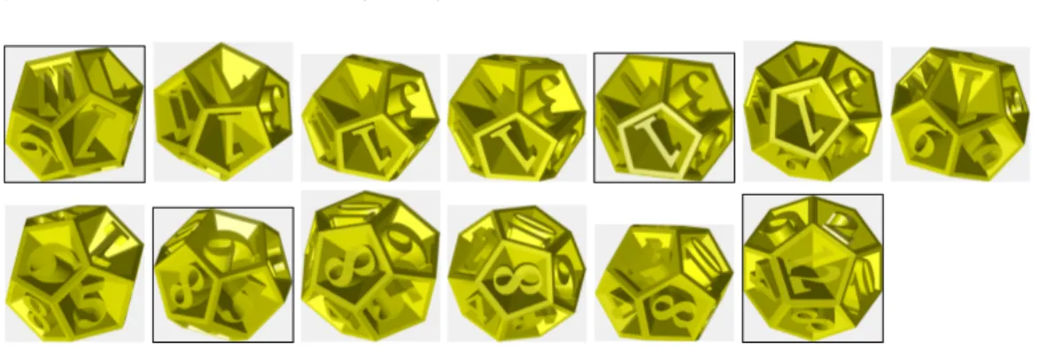
We illustrate the proposed method to construct a smooth interpolating path on SO(3) from four rotation matrices R1, R2, R3, and R4. We display the result in Figure 1 where

rotations are applied to rotate a 12 sided dice and the given time instants are displayed in a box. We can easily check that the resulting curve path is smooth including at the interpolation points.

4 Conclusion

In this paper, we have introduced a new framework and algorithms to study the fitting problem of C2 _{Bézier curves to a finite set of time-indexed data points on the special}

orthogonal group SO(n). The proposed method takes into account the global symmetries defined in the joint points. Therefore, the presented approach is valid on any locally

(9)

Fig. 1: Example of an interpolating path on SO(3) applied to rotate a 12 sided dice at given time instants (1, 5, 9, 13).

symmetric space and other Riemannian symmetric spaces. In the future, we intend to extend the theory and then apply it to more general nonlinear manifolds.

References

1. Adams, F.: Lectures on Lie Groups (1982)

2. Arnould, A., Gousenbourger, P., Samir, C., Absil, P., Canis, M.: Fitting smooth paths on riemannian manifolds: Endometrial surface reconstruction and preoperative mri-based nav-igation. In: Geometric Science of Information. pp. 491–498 (2015)

3. Barr, A., Currin, B., Gabriel, S., Hughes, J.: Smooth interpolation of orientations with angular velocity constraints using quaternions. ACM Siggraph Comput. Graph. 26, 313–320 (1992)

4. Camarinha, M., Silva Leite, F., Crouch, P.: Splines of class Ck_{on non-euclidean spaces. IMA}

J. Math. Control Inf. 12(4), 399–410 (1995)

5. Fang, Y., Hsieh, C., Kim, M., Chang, J., Woo, T.: Real time motion fairing with unit quaternions. Computer Aided Design. 30, 191–198 (1998)

6. Ge, Q., Ravani, B.: Geometric construction of bézier motions. ASME J. Mech.Des 116, 749–755 (1994)

7. Hart, J., Francis, G., Kaufman, L.: Visualizing quaternion rotation. ACM Trans. Graph. 13(3), 256–276 (1994)

8. Helgason, S.: Diﬀerential Geometry, Lie Groups, and Symmetric spaces (1978)

9. Nielson, G., Heiland, R.: Animated rotationsusing quaternions and splines on a 4d sphere. Program. Comput.Software 18(4), 145–154 (1992)

10. Popiel, T., Noakes, L.: Bézier curves and c2 interpolation in riemannian manifolds. J. Approx. Theory 148(2), 111–127 (2007)

11. Samir, C., Adouani, I.: C1_{interpolating bézier path on riemannian manifolds, with}

applica-tions to 3d shape space. Applied Mathematics and Computation 348, 371–384 (2019) 12. Shoemake, K.: Animating rotation with quaternion curves. ACMSIGGRAPH’ 85(19), 245–

254 (1985)

13. Zefran, M., Kumar, V., Croke, C.: On the generation of smooth three-dimensional rigid body motions. IEEE Trans. Robot. Autom. 14, 576–589 (1998)