HAL Id: halshs-00552981
https://halshs.archives-ouvertes.fr/halshs-00552981
Preprint submitted on 6 Jan 2011
HAL is a multi-disciplinary open access
archive for the deposit and dissemination of sci-entific research documents, whether they are pub-lished or not. The documents may come from teaching and research institutions in France or abroad, or from public or private research centers.
L’archive ouverte pluridisciplinaire HAL, est destinée au dépôt et à la diffusion de documents scientifiques de niveau recherche, publiés ou non, émanant des établissements d’enseignement et de recherche français ou étrangers, des laboratoires publics ou privés.
Deforestation in the Brazilian Amazonian Forest
Sébastien Marchand
To cite this version:
Sébastien Marchand. Technical Efficiency, Farm Size and Tropical Deforestation in the Brazilian Amazonian Forest. 2011. �halshs-00552981�
Document de travail de la s ´erie
Etudes et Documents
E 2010.12
Technical Efficiency, Farm Size and Tropical Deforestation
in the Brazilian Amazonian Forest
S ´ebastien Marchand∗
April 2010
∗
Centre d’Etudes et de Recherches sur le Developpement International (CERDI-CNRS), Universit´e d’Auvergne. 65, Boulevard F. Mitterrand, 63000 Clermont-Ferrand, France. Tel: (+33) 4 73 17 75 07, Fax: (+33) 4 73 17 74 28. E-mail address: Sebastien.Marchand@u-clermont1.fr. I would like to thank Pascale Combes-Motel, Louis-Marie Philippot and participants to seminar at University of Clermont-Ferrand (CERDI) and to the workshop on tropical deforestation held
Technical Efficiency, Farm Size and Tropical Deforestation in the
Brazilian Amazonian Forest
S ´ebastien Marchand
Abstract
This paper analyses the impact of farm productivity as well as farm size on deforestation in Brazil. A two step econometric approach is adopted. A bootstrapped translog stochastic frontier that is a posteriori checked for functional consistency is used in order to estimate technical efficiency of which estimates are introduced in a land use model to assess the impact of productivity and farm size on deforestation. Analysis of agricultural census tract data suggests that technical efficiency has a non-linear (convex) effect: less and more efficient farms use more land for agricultural activities and so they have a positive effect on deforestation. However, the majority of farms are on the ascendant slope so that efficiency implies more deforestation in Brazilian Legal Amazon. Moreover, farm size has a robust negative effect on deforestation. Contrary to many studies, this result suggests that small farms convert more natural (forested) land into agricultural land than large ones.
Keywords: Tropical deforestation, Productivity, Farm size, Stochastic frontier model, Land use
model, Brazil.
1
Introduction
The depletion of the Brazilian forest has drawn attention for a long time and been the subject of numerous studies (Pfaff,1999;Andersen et al.,2002;Chomitz and Thomas,2003;Margulis,2004; Araujo et al., 2009; Pacheco, 2009a). This is of particular importance since most Brazilian policy makers are aware that Brazil’s future is closely linked with environmental issues. To date, serious concerns exist that are related to the loss of biodiversity, climate change, local ecological disturbances as degradation of fresh water source or degradation of soil fertility and erosion (Soares-Filho et al., 2006;Salati et al.,2007).
The literature devoted to deforestation drivers allows distinguishing three categories of factors (Geist and Lambin, 2002).The first one is related to ”underlying causes”. In this category, demo-graphic factors (Southgate et al., 1990; Cropper and Griffiths, 1994), macroeconomic factors (Ar-cand et al., 2008), income levels (Bhattarai and Hammig, 2001; Culas,2007), income distribution (Koop and Tole,2001), technological factors, government policies (Andersen and Reis, 1997; Mar-gulis,2004;Pacheco,2006;Bulte et al.,2007) and institutional factors (Southgate and Runge,1990; Mendelsohn,1994;Deacon,1994;Barbier,2004;Araujo et al.,2009) as well as cultural factors are highlighted. These factors are mainly related to economic policies and social process1.
The second causes are proximate representing ”human activities or immediate causes at local level” (Geist and Lambin, 2002, p.143). Infrastructure extension (Pfaff, 1999; Margulis, 2004; Pfaff et al., 2007; Kirby et al., 2006), agricultural expansion (Angelsen, 1999), cattle ranching activities (Caviglia-Harris, 2005), agricultural income diversification (Perz, 2004), community’s management schemes (Alix-Garcia et al.,2005), wood extraction and commercial logging (Otsuki et al.,2002) are considered as proximate sources of deforestation.
Besides, intermediate causes condition the relationship between proximate and underlying causes. These intermediates ones are considered as pre-disposing environment factors i.e geographical fea-tures (rain, soil quality, forest fragmentation...)(Chomitz and Gray,1996;Chomitz and Thomas,2003; Margulis,2004;Kirby et al.,2006;Pfaff et al.,2007).
This paper contributes to the economic inquiry on the drivers of deforestation at the farm level2
1
Barbier and Burgess(2001),Angelsen and Kaimowitz(2001) provide an exhaustive review of the literature. 2Browder et al.(2004) provide a review of the literature on determinants at farm level (Pich´on,1997;Godoy et al.,
1997) according three different models: the neoclassical economic tradition (NET), the household life cycle (HLC) (Walker and Homma,1996;Perz and Walker,2002) and the political ecology approach. Our study is more linked to the first model in which a farmer manages his production in order to maximize his utility under some constraints and so agricultural
and goes beyond existing literature by examining whether there exists a clear and unambiguous link between agricultural efficiency and deforestation. Put differently the question is whether efficient agri-cultural producer in the Amazonia have also sound environmental practices. Many papers analyse the effect of efficiency and reveal that inefficient farms (i.e with an extensive production) deforest more without estimate empirically the effect of productivity (Otsuki et al.,2002;Bulte et al.,2007;Keil et al.,2007). For example,Godoy et al.(1997, p. 978) explain that an ”increase [of] the productivity of land (...) create(s) incentives to cut less forest”. However, a potential increase of productivity can create incentives to cut more tree if an efficient farm is in a context of relatively poor valorisation of the environment. The main idea of this paper is to show that an efficient producer can increase its propensity to deforest because he does not take account the environment so that cleared land costs are low. Therefore, this kind of farmer increases an activity in which he is efficient i.e agriculture and so deforests (Boserup,1965;Angelsen,1999). Angelsen(1999) explains theoretically that in an open economy and an open access model3, an increase in output productivity enhances agriculture
expansion i.e deforestation. Besides, Pacheco(2009b, page 40) argues that ”wealthier farmers not only tend to deforest more in absolute terms but also show a slightly greater propensity to deforest whatever their production system” by using a clustering analysis and creating a wealth index4. In
other words, producers exploit extensive margins when they exist, before turning to intensive mar-gins. Therefore, this study estimates econometrically a potential impact of productivity on agricultural expansion i.e on deforestation. To our knowledge, onlyJones et al.(1995) have analysed empirically this effect in the Brazilian context. They find that the stock of cleared land is lower in farms with a higher productivity in cattle and cultivated land but that productivity has no effect on the pace of cleared land (Jones et al.,1995, p.179-180).
Several studies also analyse the effect of farm size on deforestation at the farm level and often conclude on a positive effect of farm size. Walker et al. (2002) compile results from 15 farm level models and find that the farm size has a positive effect on deforestation. This link is however indirect since there exists a correlation between farm size and agricultural land use (Browder et al.,2004). For example, there is often a positive correlation between specialized production systems like cattle
variables (like productivity, farm size, output composition). 3
In this model (his model four), there is an open access regime and property rights are defined by forest clearance. This model is particularly well-defined for the Brazilian context (Angelsen,1999, page 190).
4This index is derived from three measures (the number of cattle, number of lots of land, and property size in hectares) and two indices (an index of equipment and an index of durable goods owned by the household). However, the concept of wealthy is particularly large and our study only puts forward the effect of productivity and farm size.
production with farm size implying a positive correlation between farm size and extensive production. Pacheco (2009a) finds also that smallholders tend to less deforest than medium-large-scale ones because these small farmers have diversified their incomes. In others words, the relation between farm size and deforestation is linked with production systems. To our knowledge, there is no estimate of the marginal effect of property size on the agricultural use of land owned by a farmer i.e when the production system is controlled.
The effect of agricultural productivity and farm size on deforestation is estimated on census-tract-level data from the Censo Agropecuario 1995-96. This census permits to analyse the behaviour of each farm present in the Legal Amazon5 between 1995-1996 and to avoid an aggregation bias. In fact, these data allow to estimate the level of technical efficiency thanks to dis-aggregated data on agricultural activities. Then, to assess the link between deforestation and productivity, a two step method is implemented. In the first step, technical efficiency is estimated from a stochastic production frontier model (Aigner et al.,1977). Secondly, in the second stage, the estimated technical efficiency is considered as a determinant of deforestation as well as farm size in a land use model following Chomitz and Gray (1996) and Chomitz and Thomas (2003). Moreover, in this model, effects of determinants of land use are studied so we equate an increase in agricultural land with deforestation. The paper is organized as follows. Section 2 briefly describes the Legal Amazon and its historical background. Data, the stochastic production frontier model and the land use model are discussed in section 3. Section 4 analyses the econometric results followed by a conclusion in section 5 which discusses the main results and tries to bring some explanations linked to Brazilian context.
2
Tropical deforestation and agricultural technical efficiency:
back-ground
The Brazilian Legal Amazon (BLA) is an administrative area, created in 1953 to reduce the relevant economic, demographic and natural heterogeneities in Brazil6: the BLA has 20 million inhabitants
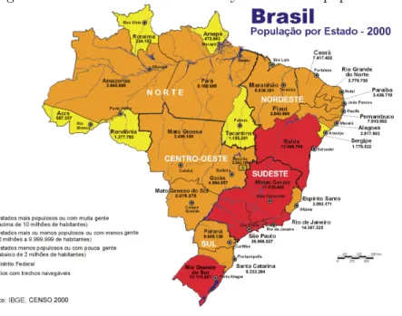
of the 170 millions Brazilians in 2000 (source: IBGE ; see figure1, page 23) on more than half of the territory. This demographical heterogeneity was more important before the implementation of
5This administrative area was created in 1953 and regroups nine states which are Acre, Amazonas, Amapa, Para, Rond˜onia, Roraima and Tocantins (North region), Mato Grosso (Center-West region) and Maranh˜ao (North-East region). 6An important heterogeneity of population within the BLA is also highlighted. Para and Maranh˜ao concentrate more than half of the population (10 millions (source: IBGE, see figure1, page23).
development policies, since the 60s. The BLA population represented 8% of the total population in 1970 while it was of 12% in 2000. The demographical growth of BLA was more important mainly as a result of development policies.
In the 60s, the military government begun to considered economic and political objectives. The main one was a military and strategical one to discourage as well incursions from neighbours that the formation of domestic guerilla opposition. However, the second incentive was to provide land to people landless peasant in order to deal with demographic pressures.
Development policies have consisted in building of roads, colonization and land titling projects. The regional development policies of the Amazon Legal started in 1966 with the first phase called ”Operation Amazonia”. There are seven phases and the last one, Avanc¸a Brasil, started in 2000 with the aim to conciliate development and environment7. However, the regional development policy has been very criticized because of important resulting deforestation. As a consequence of this policy some 35 million ha were deforested between 1970 and 1995. In mid-nineties, nearly 10 percent of the BLA area was deforested, compared to 2.5%, in 1975. During this period, the growth of deforestation was 18 000 km2 per year. More recently, the last phase was particularly criticized.
Indeed, according to the Brazilian National Institute of Space Research (INPE, Instituto Nacional de Pesquisas Especiais), the annual cleared area increased from 18 226 (in 2000) to 27 379 km2 (in 2004)8. However, since 2005, an improvement can be noticed as the annual cleared surface decreases: from 18 759 (2005) to 11 224 km2(2007).
Another important issue in the Brazil Legal Amazon is the very uneven land distribution. The pres-ident Fernando Enrique Cardoso (1995-2002) implemented a proeminent agrarian reform continued by the president Lula since 2002. This reform consists in ”maintaining and stimulating a modern agricultural sector that finally produced for the best interests of the larger society, while using welfare programs, including land reform, to ameliorate the worst social effects of agricultural modernization and provide some relief to a conflict-ridden countryside” (Pereira,2003, p.48). The policy’s aim was to modernize agricultural sector by allowing landless or small landowners to have or secure land. In others words, this agrarian reform tried to secure property rights which can reduce deforestation (Araujo et al.,2009).
7
These phases were implemented between 1971 and 2000. The second, third and fourth step (during the 70s and 80s) aimed to increase the regional development by colonization and big infrastructure projects. The nineties phases were oriented toward more environmental considerations.(Andersen et al.,2002, Chap. 2).
Recently, the Brazil’s climate change plan, adopted in 2008 and implemented in 2009 by president Lula, implies to reduce global warming by stimulating high efficiency, maintaining a high proportion of renewable energy in the electricity production, encouraging the use of biofuels in the transportation sector, and reducing deforestation. In this last issue, the goal is drastically downsize illegal deforesta-tion and then to eliminate the net loss forest in 2015 (a tree planted for a tree cut).
The Brazilian regional development policy have influenced the economical behaviour of farmers. However, the question is not so much whether this policy has increased agricultural efficiency but rather how this policy has changed conditions i.e if the opportunity cost associated with agricultural activities has been modified by regional development policies. By the way, beyond to increase de-forestation by colonisation project, road networks or infrastructure projects, regional development policies affect agricultural productivity by influencing the agricultural modernization and the relation between agricultural inputs (Reis and Blanco,1997). Several channels can be highlighted to explain this effect. For example, the improvements in market accessibility, lower rural wages or a reduction of agricultural prices inputs (like fertilizer, credit availability) modify profitability of agricultural option as well as the degree of substituability/complementarity of inputs. Firstly, these changes can en-hance extensive shifting cultivation and so deforestation because of agricultural activities are more profitable than conservative forestry activities. Secondly, for example, an efficient farmer, with no constraint to achieve their labor and capital inputs, can increase their land use in order to improve his profitability given that natural environment is less valorized. In this case, more efficiency can increase deforestation because of land is a complementary of labor and capital. In a more valorized environ-ment context, land is less used whereas labor and capital can be increased for an efficient farmer. Therefore, the intensive margin will be use before the extensive one in this context (Angelsen,1999). However, it is not the Brazilian case with a less valued natural environment and an open access to land.
3
Methodology and conceptual framework
3.1 The 1995-1996 Censo Agropecu´ario
The dataset come from the Censo Agropecu ´ario that was conducted in 1995 by the Brazilian Institute of Geography and Statistics (IBGE-Instituto Brasileiro de Geografia e Estat´ıstica). The census used
covers the Legal Amazon (BLA) made up of all the states in the Northern region of Brazil plus parts of the states of Maranh ˜ao and Mato Grosso (see1, page23).
However some states are fully covered by tropical forest (like Amazonas and Acre States) and other are partially covered by tropical woods (Mato Grosso and Maranh ˜ao). However, every agricul-tural conversion of a naagricul-tural area is considered as deforestation. Therefore, a farm in Mato Grosso which converts a savannah area in an agricultural area has the same impact on deforestation that a farm in Acre which converts a tropical forest area into an agricultural area. More precisely, there is the same impact in terms of biodiversity but not in terms of cleared trees (Angelsen,1999;Andersen et al., 2002). In other words, as noted by Angelsen (1999, pages 187-188), the model ”implicitly assume that all agricultural expansion takes place into forested areas, which in reality is not the case. Thus in empirical work one should not equate an increase in agricultural land with deforestation. Nev-ertheless, agricultural expansion is the main source of deforestation, and is therefore worth studying for understanding the causes of deforestation”9.
Besides, the dataset consists in ”representative farms” which encompass farms which have the same size (15 types of size) and land tenure (owner, sharecropper, renter or occupant) located in one county. 893 129 farms are regrouped in 14 724 ”representative farms” involving an average of 61 farms per ”representative unit” (Chomitz and Thomas,2003;Helfand,2004).
3.2 Estimated technical efficiency with a stochastic production frontier model
In order to estimate productive efficiency, a production function is used i.e only technical efficiency is analysed10. A non-optimal use of production factors which can be put forward for agricultural
Brazilian farmers (constraints on labor and credit markets are strong) implies a technical inefficiency well-known as X-inefficiency (Leibenstein,1966).
Considering that a producer i uses multiple inputs X to produce a single or a multiple output Y , a production function can be written to represent a particular technology: Yi = f (xi), where f (xi)is
called a production frontier. On the frontier the producer produces the maximum output for a given set of inputs or uses the minimum set of inputs to produce a given level of output. In standard
9
Andersen et al.(2002, P.12-13) point out that ”transitional areas are just valuable as the dense forest in terms of both biodiversity and biomass record stored”.
10
Farm productivity can be generally decomposed into two elements: a dynamic and a static one. The first element is related to technical progress and the second one to productive efficiency. To analyse the first element, it is necessary to have time series. Our data set does not allow us to have a temporal dimension so only farm’s productive efficiency may be analysed. In fact, the 1985 census could have be used to have a temporal dimension but the 1995 census was completely different from previous census (seeAndersen et al. 2002, p.45-47 for more details).
microeconomic theory there is no inefficiency in the economy implying that all production functions are optimal and all firms produce at the frontier. But if markets are imperfect, producers can be pulled beneath the production frontier.
An ouptut-oriented measure of technical efficiency (more output with the same set of inputs) gives the technical efficiency of a farmer i as follows:
T Ei(x, y) = [max φ : φy ≤ f (xi)]−1 (1)
The parameter φ is the maximum output expansion with the set of inputs xi.
An ouptut-oriented measure of technical efficiency is estimated under three auxiliary hypothesis. Firstly, equation1is applied into an econometric model as (Kumbhakar and Lovell,2000, p.64):
Yi = f (Xi; β).e−Ui (2)
where Yiis a scalar of output, Xia vector of inputs used by the producer i = 1, ..., N and f (Xi; β)
is the production frontier11 where β is a vector of technology parameters to be estimated. U i are
non-negative unobservable random variables associated with the technical inefficiency of production which follows an arbitrary distribution12.
Secondly, a stochastic production frontier is used (Aigner et al., 1977; Meeusen and van den Broeck,1977) so that the error term has two components: random shocks Vi (not attributed to the
relationship between inputs and output) and the inefficiency Ui13. Therefore, the equation2becomes:
Yi = f (Xi; β).e−Ui.eVi (3)
Where Vi represent random shocks which are assumed to be independent and identically distributed
with a normal distribution, mean zero and unknown variance. Under that hypothesis, a producer beneath the frontier is not totally inefficient because inefficiencies can also be the result of random shocks (like climatic shocks).
11
The production frontier has the traditional properties of monotonicity, continuity and concavity (Fuss and McFadden,
1978, p.226-227).
12We choose alternatively the half-sided normal distribution or the exponential one. 13
A deterministic frontier implies a one way error term which is the inefficiency. The gap to frontier is only due to inefficiency.
Since T Eiis an ouptut-oriented measure of technical efficiency, a measure of T Eiis: T Ei = P rodobs P rodmax = f (Xi; β).e −Ui.eVi f (Xi; β).eVi = e−Ui (4)
The technical efficiency is, then, estimated using the stochastic frontier model given by the equa-tions3and4.
Thirdly, the production function is modelled using a transcendental logarithmic (”Translog”) spec-ification. The translog specification is preferred to a Cobb-Douglas form (Diewert,1971) because of its flexibility implying no restrictions on coefficient’s substitutability (factor substitutability is equal to one in a Cobb-Douglas case)14.
The traditional translog specification used follows the general form15(Christensen et al.,1971):
ln(Yi) = β0+ 4 X j=1 βjln(Xij) + 1 2 4 X j=1 4 X k=1 βjkln(Xji)ln(Xki) − Ui+ Vi (5)
Where i = 1, ..., N are the farmer unit observation; j, k = 1, 2, ..., 4 are the applied inputs; ln(Yi)is
the logarithm of the output of the farmer i and ln(Xij)is the logarithm of the jtm input applied of the
ithindividual; and βj, βjk are parameters to be estimated16.
The final empirical model estimated in the translog case is
Outputi,c= β0+ β1.Labori,c+ β2.Landi,c+ β3.Livestocki,c+ β4.P urchasedi,c
+β5.Labori,c2 + ... + β9.Labori,c∗ Landi,k+ ... + λ − Ui,c+ Vi,c
(6)
Which represents the relationship between output and inputs for the producer i in the county (munic-ipality) c and where λ is a state fixed effect.
The output is an aggregated output variable of three categories: animal production (cattle, chick-ens,...), harvest production (soybean, corn, coffee...) and plant production (wood,...). It is the gross value of agricultural output (for more details see annex B.1)17(Helfand,2004).
14
A likelihood ratio test (LR) was implemented in order to test the functional form of the production function. In all tests, restrictions can be rejected at a very low confidence level so that the translog specification can be preferred. Details available upon request.
15We use a negative sign in order to show that the term −Uirepresents the difference between the best efficient firm (on the frontier) and the observed firm.
16
Similarity conditions are imposed i.e βjk= βkj. Moreover, production frontier requires monotonicity (first derivatives i.e elasticities between 0 and 1 with respect to all inputs) and concavity (second derivatives negatives). These assumptions should be checked a posteriori by using the estimated parameters for each data point.
Four inputs are taken into account18. The variable Labor includes all the persons who work in the farm. There are both family and hired labor and all are measured in full-time equivalent unit. The input Stock lives is the stock of animals in cattle equivalents. Land represents the total area (in hectares) held by a farm. All kind of land were aggregated: crops, pasture, productive land that was not being used (fallow) but also land which was not used for agricultural issue (forest, woodland and useless land). AsHelfand(2004), Purchased inputs are the expenditures of feed and medicine for animals, fertilizer, chemicals (such as pesticides and herbicides), seeds and fuel19.
However, a survey data is used and there can be proximity effects implying a correlation between producers behaviours in a same area. Therefore, error terms are correlated so that standard errors and the analysis of the significance of coefficients are biased. To avoid this potential spatial correlation between farms, errors terms are bootstrapped (200 replications) (Wooldridge,2002, p. 378-379).
3.3 A land use based deforestation model
The analysis of deforestation is done following the land conversion model ofChomitz and Gray(1996). The basic assumption of this model is that a farmer allocates his plot either to an agricultural activity or leave it uncleared i.e under forest20.
In other words, the propensity to clear land i.e the proportion of deforested land (p) depends on the potential profits (π(X)) per hectare from converting the natural land to agricultural use. Potential profit depends on X, a vector of farm level explanatory variables.
A traditional structural form of this model is the tobit (Chomitz and Gray, 1996; Dolisca et al., 2007):
p∗i,c = αXi,c+ ϑi,c (7)
Where p∗i,c is the latent dependent variable of farmer i in the county c explained by Xi,c, a set of
explanatory variables influencing the potential profit. α = (α1...αk)0is a vector of unknown parameters
and ϑi,c is the error term. The dependent variable is latent i.e it cannot be observed for p∗i,c < 0, so
18For more details, see descriptive statistics in table4, page26and annexBfor Labor and Stock lives inputs. 19
The number of tractors (in equivalent 75 hp) had been introduced but removed given that it does not respect theoretical assumptions of monotonicity and concavity. However, results do not change with this input. Results available upon request.
20
The use may be agricultural (annual or peri-annual harvest, livestock, fallow or planted forest) or natural (the land remains natural i.e natural forest or natural pasture).
we have,
pi,c = 0 if p∗i,c ≤ 0
pi,c= p∗i,c otherwise
where pi,c is the observed dependent variable.
In other words, farmers with unprofitable areas belong to the same group so that the observed dependant variable is censored at 0.
Finally, the estimated model is:
pi,c = α0+ α1T Ei,c+ α3T Ei,c2 + α4Sizei,c+ α2Xi,c+ εi,c (8)
Where pi,c is the observed dependent variable defined by the agricultural land ratio of farmer i
in the county c. This is a ratio between agricultural land use (crops, cattle, planted pasture, short fallow) and all land uses. A ratio equals to 1 involves that a farmer uses all his land for agriculture. T E is technical efficiency estimated from stochastic production frontier model. Size represents the average size of each individual farm in the representative farm. It is a coded variable defined in the table 2, page 2521. X regroups a set of covariates in four categories22: land tenure (owners
(62 percent), sharecroppers (26 percent), renters (9 percent) and occupants (3 percent), see table
3, page 25for more details), output composition (peri-annual crops, annual crops, plant production, animal,...), public goods (cooperative, financing, technical assistance and electricity) and the last category focuses on technology (artificial insemination, irrigation, soil conservation, ...). This last category allows to control for some credit and capital market imperfections.
The expected sign of the coefficient of efficiency is difficult to highlight. The literature often con-cludes that an intensive farm deforests less that an extensive one but in the Brazilian case, even an efficient farm can exploit the extensive margin before the intensive margin. In other words, a more efficient agricultural unit deforests more than a less efficient one. Hence, the sign of this coefficient can be positive. However, if the sign is negative (other things equal, including agricultural land), it is expected that increasing efficiency curtails deforestation. In other words, an inefficient farm would have an extensive production.
21
I dropped all farms in the 16th code (only 0,02 percent of all farms) because these farms do not declare their size. 22For more details, see descriptive statistics in table4, page26.
However, the relationship between technical efficiency and deforestation may be non-linear and convex. Indeed, a poorly efficient farm compensates for these inefficiencies by increasing abundant factors, i.e land. However a more efficient farmer can use this efficiency to invest and acquire new land. The non-linear effect is introduced with the term T Ei2 and α3 represents the non-linear effect
of the technical efficiency. A positive sign induces a convex effect and therefore a strong effect on deforestation both when efficiency (inefficiency) is low (high) and high (low). The relevant question is actually whether an efficient farmer with an intensive production will stop his expansion or accelerate deforestation (Angelsen and Kaimowitz,2001) and so if he exploits extensive margins when there exist, before turning to intensive margins. This kind of situation can occur in the Brazilian case char-acterized by an open economy and an open access to land in which an increase in output productivity enhances agriculture expansion i.e deforestationAngelsen(1999).
α4measures the size effect which is expected to be negative. Indeed, a small farm can have a high
discount rate involving a great agricultural land use23. Agricultural producers use the most abundant
factor if they are constraint in the use of other factors (Boserup, 1965; Angelsen and Kaimowitz, 2001). Moreover, other interesting explanation of this negative effect can be found in the specific Brazilian context of land distribution. In BLA, a very important inequality in land distribution driven by a political scheme can explain this negative effect. Some authors (Pereira,2003;Andersen et al., 2002) put forward this great heterogeneity in land distribution. In fact, large farmers can receive lands from the state without paying from them, then they receive fiscal incentives to produce, but they produce anything and they simply hold the land without paying from them (Pereira,2003, p.56). In this context, small ones have to acquire land titles by developing the land, living on it, and cultivating it (Andersen et al.,2002, p.32).
However, there is an other important issue: the abundance of land. The idea is that farmers convert their forested plots because lands are very abundant and open accessed. Boserup (1965) emphasizes this idea to explain the drop in deforestation in Europe. County fixed-effects are intro-duced in order to control for the abundance of land. Moreover, transportation cost as well as climate features (precipitation levels) are controlled by these municipios fixed-effects.
4
Results
4.1 Technical efficiency estimation
The first part of the study concerns the econometric estimation of technical efficiency with a translog specification common to all farmers. In other words, the technology used and the technical relation-ship between inputs and output(s) are supposed to be the same for all farmers.
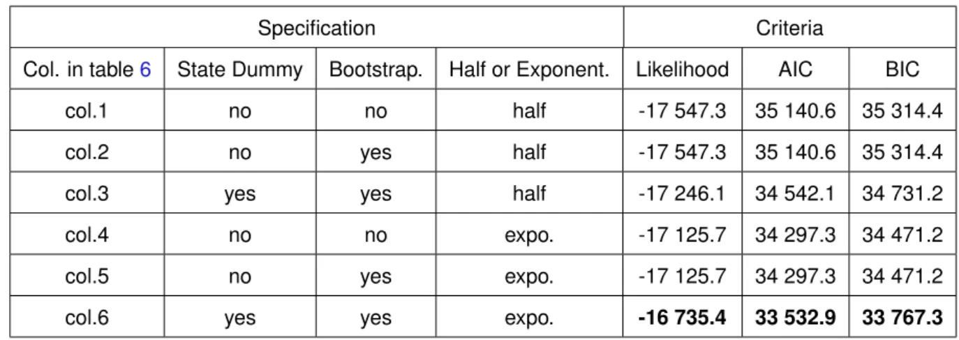
The maximum likelihood estimator is used to estimate technical efficiency with Stata 10 and the command frontier. We use two possible distributions for efficiency : a half-normal law (col.1 to 3 table
6, page28) and an exponential law (col.4 to 6 table6, page28). Standard errors are corrected by bootstrapping (200 iterations). State fixed-effects are controlled with state dummies. The aim of this step is to estimate efficiency in order to use it in a second step. Therefore, technical efficiency has to be significant.
[see table6, page28around here]
The first result is the significance of technical efficiency in all regressions. In other words, the model seems to be relevant to analyse and use technical efficiency as a regressor in the land use model. Indeed, if the estimated efficiency had not been significant in the stochastic frontier model, our specification would have been imperfect. Moreover, the share of efficiency ”half-normal” in the random deviation is more important than the share of efficiency ”exponential”. In order to deal with this heterogeneity, Spearman’s rank correlation coefficients are used. We want to determine if the choice between these distributions is important. The Spearman’s coefficient between efficiency esti-mated by a half-normal distribution and by an exponential one is 0.99 so that these two estimates of efficiency are very close. However, an analysis of descriptive statistics of efficiency reveals that the average is 0.56 with a half-normal distribution and 0.66 with an exponential distribution. This result suggests a substantial difference in means. Therefore, the choice of the distribution of efficiency can influence the results of the land use model. In order to choose between an half-normal distribution and an exponential one, we run two measures for comparing maximum likelihood models. These two measures are the Akaike Information Criterion (AIC) and the Bayesian Information Criterion (BIC). In all specifications (i.e with or without state dummies, bootstrapping or not), the exponential distribution is preferred to the half-normal one (see table5, page27)24.
24
[see table5, page27around here]
The second important step is to analyse the relevance of our model. Hence, we check the theoret-ical consistency of our estimated efficiency model by verifying that marginal products are positive and decreasing (monotonicity). In other words, if these theoretical criteria are jointly empirically validated, then the obtained efficiency estimates are consistent with microeconomic theory and can be used as determinant in the land use model.
As the coefficients of the translog functional form allow no direct interpretation25 in the magni-tude and significance of individual output elasticities, the latter were computed for all inputs at the sample mean (from coefficients of col.6). Brazilian agricultural production depend more strongly on purchased inputs (0.65) and labor (0.39). These findings suggest that efficiency gains are most likely with respect to purchased inputs and labor. The total contribution of production factors is more than 1 (1.02) implying increasing return to scale.
Finally, the model seems to be correctly specified because the returns to scale are positive (in all specifications) and the condition of monotonicity seems to be respected26. In other words, the production technology and the inputs used are relevant. Hence our specification seems to be good and we can suppose that the technical efficiency estimated is appropriated because this element is in fact the part not-explained by the model
4.2 Land use determinants
Two statistical problems linked to spatial correlation and generated regressors must be considered. Firstly,Deaton(1997) brings spatial correlation into light when survey data are used. Indeed, house-holds in a single cluster (for example the county) live near one another, and are often interviewed at the same time (survey teams are often in one county at the same time). Moreover, farmers in a same county are engaged in the comparable agricultural activities because comparable soil qualities, pests or weather effects as well... Estimations are thus amenable to this spatial correlation: inefficient
25It is important to note that the coefficient estimated in the translog specification is not the input’s elasticity and so the result cannot be easily interpreted as in the constant-elasticity Cobb-Douglas case. In others words, the elasticities of mean output with respect to the jthinput variable is calculated at the means of the log of the input variable and their second order coefficients as follows:
δlnY
δXj = βj+ 2.βjjlnXj+ Σ 4
j6=kβjklnXk (9)
.
26However, at the mean sample, the marginal productivity of size is negative. This result does not validate the theoretical predictions but seems to be relevant. In fact, land is more a political or illegal attribute than an economic input in the brazilian case suggesting that it does not contribute normally to agricultural production.
estimation may be suspected. A clustering approach allows to consider that all farmers in the same county are spatially correlated. So, we deal with the similarity between people within the same cluster (municipality). In addition, county fixed effects are used.
For the second problem, the use of the estimated technical efficiency creates a potential gen-erated regressor bias which could bias the estimate of the standard errors downward and so the estimation is not efficient. However,Pagan(1984) (theorem 7, page 233) show that estimates of the variance of residuals used like regressor (here technical efficiency) are correct27. In other words, the
standard errors of technical efficiency are efficient and ”t-statistic are ”right”.
[see table7, page29around here]
The first column consider only a linear effect of technical efficiency which follows an exponential law in the first column28. Productivity has a positive and significant effect so that more efficient farms convert more natural plot into agricultural land29. The size has a negative and significant effect.
The second column does not consider county fixed-effects but introduces anon-linear effect of
efficiency. Efficiency2has a positive and significant coefficient at the one percent level and Efficiency
is negative so that these results imply that there is a convex-effect of productivity on deforestation. Size effect does not change. A substantial result of this regression is that agricultural conversion is not driven by state fixed effects and so by natural areas surrounding farms. In other words, the proeminence of the stock of natural forested land does not condition the effect of productivity and farm size on agricultural expansion.
The third column is our preferred specification and considers a non-linear effect of efficiency. The results remain the same concerning the convex effect of efficiency and the negative effect of size. The quadratic term has a positive and significant coefficient at the one percent level i.e a convex effect of technical efficiency on deforestation. An increase of 1 percent of efficiency induces an increase of nearly 0,02 percent of the agricultural ratio30. Moreover, an increase of 10 percent of the
27
Two conditions are necessary. The first one is that the residuals of the two equations are independent and the second is that the predicted variable in the first equation is not used (here the predicted output).
28To further test the robustness of my results, an another estimator was used: the quantile regression estimator. Standard errors are bootstrapped in order to avoid the spatial correlation problem. The convex-effect of productivity is robust to this change of estimator as well as the negative effect of farm size. Those results are not presented here but they are available upon request.
29Efficiency as well as efficiency2 can be endogenous. To avoid this potential problem, we did some Spearman’s rank correlation coefficients between efficiency and the residuals of each regression. In the majority cases efficiency (and so efficiency2) is independent of the residuals (details available upon request).
30We have at the mean efficiency, δratio
δef f iciency = δef f iciency+2×δef f iciency
2= −0, 228+2×0, 186×ef f iciency = 0, 02 where coefficients are elasticities.
mean efficiency (from 0.66 percent to 0.73 percent) implies an increase of nearly 0.86 percent of the agricultural ratio in the translog specification31. Further, the reversal point is obtained for an efficiency of 61 percent so that there is an optimal efficiency allowing to reduce deforestation32. Moreover, only 25 percent of farms have an efficiency lower than 61 percent. In other words, many farms are on the ascendant slope which implies actually that more efficiency induces more agricultural use of natural plot. Besides, farm size has a robust negative effect. In this specification, a one standard deviation average increase in farm size decreases dependent variable of 0,03.
In the column four, technical efficiency estimated from a half-normal law is introduced. The effect of size remains strongly negatively significant and the non-linear effect of efficiency remains positive and significant.
Finally, in all regressions, renters, sharecroppers and illegal occupants convert more natural land than owners. This result implies that property rights allow to reduce deforestation i.e an owner is more likely to implement more long term activities. Temporary crops and cattle activities (Caviglia-Harris, 2005) are the two main types of production to contribute to deforestation. Lastly, the cooperative and the funds received (Margulis,2004) seems to reduce the agricultural pressure on natural land.
5
Conclusion
The aim of this paper is to assess the effect of farm productivity and farm size on deforestation using a census-tract-level data from the Censo Agropecuario 1995-96. This census allows us to analyse the behaviour of each farm present in Legal Amazon between 1995-1996. Besides, a two step approach is implemented to assess this link. The first one is to estimate the productivity with a stochastic production frontier model which allows to assess the technical efficiency of each ”representative farm”. In the second step, this estimated efficiency is introduced in a land use model in order to study determinants of deforestation at farm level data.
We find that productivity, approximated by an estimated technical efficiency, has a convex effect on deforestation. We can say that less and more efficient farms convert more natural plot into agricultural land. On the one hand, less efficient units can have some constraints on labour or credit market33and
31With coefficients of the column 3 of table7, page29and after transformation in order to have elasticities, we have: ∆ratio = [1.068 − 0.228 × 0.73 + 0.186 × 0.73 × 2] − [1.068 − 0.228 × 0.66 + 0.186 × 0.66 × 2] = 0.01 or an increase of 0.86 percent of the agricultural ratio.
32
Around this level of efficiency, a marginal increase of efficiency does not increase agricultural expansion.
so cannot optimally use their factors (labour and capital). This kind of farms use the more abundant factor: the land. For those farmers, the input land is a substitute of others constrained inputs. On the other hand, the more efficient farms have no constraint. They can use labor and capital optimally and so can use more land. For efficient farmers, land is a complement input of labor and capital. Moreover, the reversal point is for an efficiency ranging from 61 percent but less than 25 percent of Brazilian farmers in Legal Amazon have a productivity lower than 61 percent in 1995. Hence, the majority of farms are on the ascendant slope. This result implies actually that Brazilian farmers convert more natural land into agricultural plot when their efficiency increases. This result can be explained by the poor environmental valorization of Brazilian tropical forest and the problem of open access to land which push farmers to exploit their extensive margins before their intensive ones (Angelsen,1999).
We also uncover that a small farm converts more land than a large one. This result was expected. Indeed, a small farm has more constraints than a large one. These constraints can enforce small farms to use more land. However, since we control for the level of efficiency, these constraints can occur only on the size because the two farms have the same efficiency level. In fact, a small farmer can have a high discount rate so that he is induced to convert natural land (Boserup,1965;Angelsen and Kaimowitz,2001). The very heterogeneous context of land distribution in BLA (Pereira, 2003; Andersen et al.,2002) can explained this result. Small farmers have actually not the right political connections to acquire land so that they must cultivate their plots to acquire them34.
To conclude, our results can be explained by the Brazilian context. A poor environmental valoriza-tion and a very important inequality in land distribuvaloriza-tion can condivaloriza-tioned our findings. In this sense, an important improvement would be to use the new census 2005-2006 of IBGE. It would be interesting to have a temporal dimension allowing us to use more information to test the role of environmental val-orization of forest. The recent regional policy of development(Avanc¸a Brasil) can actually improve this valorization allowing efficient farmers to have an intensive production which respects environment.
References
Aigner, D., Lovell, C. A. K., Schmidt, P., 1977. Formulation and estimation of stochastic frontier pro-duction function models. Journal of Econometrics 6, 21–37.
on labor market. However, some others imperfections on credit and capital markets can occur and explain our results. 34
The Brazilian agrarian reform developed by the president Fernando Henrique Cardoso (1995-2002) starting from 1995-1996 can not be analysed with our results.
Alix-Garcia, J., de Janvry, A., Sadoulet, E., 2005. A tale of two communities: Explaining deforesta-tion in mexico. World Development 33 (2), 219 – 235, institudeforesta-tional arrangements for rural poverty reduction and resource conservation.
Andersen, L. E., Granger, C. W. J., Reis, E. J., Weinhold, D., Wunder, S., 2002. The dynamics of deforestation and economic growth in the brazilian amazon. Cambridge University Press.
Andersen, L. E., Reis, E. J., 1997. Deforestation development and government policy in the brazilian amazon: an econometric analysis. Texto para Discuss ˜ao - Ipea 513.
Angelsen, A., 1999. Agricultural expansion and deforestation: modelling the impact of population, market forces and property rights. Journal of Development Economics 58, 185–218.
Angelsen, A., Kaimowitz, D., 2001. Agricultural Technologies and Tropical Deforestation. CAB Inter-national, Wallingford.
Araujo, C., Bonjean, C. A., Combes, J.-L., Motel, P. C., Reis, E. J., 2009. Property rights and defor-estation in the brazilian amazon. Ecological Economics 68 (8-9), 2461 – 2468.
Arcand, J.-L., Guillaumont, P., Jeanneney-Guillaumont, S., 2008. Deforestation and the real exchange rate. Journal of Development Economics 86 (2), 242–262.
Barbier, E. B., 2004. Explaining agricultural land expansion and deforestation in developing countries. American Journal of Agricultural Economics 86 (5), 1347–1353.
Barbier, E. B., Burgess, J. C., 2001. The economics of tropical deforestation. Journal of Economic Surveys 15 (3), 413–33.
Bhattarai, M., Hammig, M., 2001. Institutions and the environment kuznets curve for deforestation: A crosscountry analysis for latin america, africa and asia. World Development 29 (6), 995–1010.
Boserup, E., 1965. The Conditions for Agricultural Growth: the Economics of Agrarian Change under Population Pressure.
Browder, J. O., Pedlowski, M. A., Summers, P. M., 2004. Land use patterns in the brazilian amazon: Comparative farm-level evidence from rond ˆonia. Human Ecology 32 (2), 197–224.
Bulte, E. H., Damania, R., Lopez, R., 2007. On the gains of committing to inefficiency: Corruption, deforestation and low land productivity in latin america. Journal of Environmental Economics and Management 54 (3), 277–295.
Caviglia-Harris, J., 2005. Cattle accumulation and land use intensification by households in the brazil-ian amazon. Agricultural and Resource Economics Review 34 (2), 145162.
Chomitz, K. M., Gray, D. A., 1996. Roads, land use, and deforestation: A spatial model applied to belize. The World Bank Economic Review 10, 487–512.
Chomitz, K. M., Thomas, T. S., 2003. Determinants of land use in amaz ˆonia: A fine-scale spatial analysis. American Journal of Agricultural Economics 85 (4), 1016–1028.
Christensen, L. R., Jorgenson, D. W., Lau, L. J., 1971. Conjugate duality and the transcendental logarithmic function. Econometrica 39 (4).
Cropper, M., Griffiths, C., 1994. The interaction of population growth and environmental quality. The American Economic Review 84 (2), 250–254.
Culas, R. J., 2007. Deforestation and the environmental kuznets curve: An institutional perspective. Ecological Economics 61 (2-3), 429 – 437.
Deacon, R. T., 1994. Deforestation and the rule of law in a cross-section of countries. Land Economics Vol. 70,No. 4, pp. 414–430.
Deaton, A., 1997. The Analysis of Household Survey. Washington, D.C.: Johns Hopkins University Press for the World Bank.
Diewert, W. E., 1971. An application of the shephard duality theorem: A generalized leontief produc-tion funcproduc-tion. The Journal of Political Economy 79 (3), 481–507.
Dolisca, F., McDaniel, J. M., Teeter, L. D., Jolly, C. M., 2007. Land tenure, population pressure, and deforestation in Haiti: The case of Foret des Pins Reserve. Journal of Forest Economics 13 (4), 277–289.
Fuss, M., McFadden, D. L., 1978. , Production Economics: A Dual Approach to Theory and Applica-tions Volume I: The Theory of Production. North-Holland Publishing Company.
Geist, H., Lambin, E., 2002. Proximate causes and underlying driving forces of tropical deforestation. BioScience BioScience, 143–50.
Godoy, R., ONeill, K., Groff, S., Kostishack, P., Cubas, A., Demmer, J., McSweeney, K., Overman, J., Wilkie, D., Brokaw, N., Martinez, M., 1997. Household determinants of deforestation by Amerindi-ans in Honduras. World Development 25 (6), 977–987.
Helfand, S. M., December 2004. Farm size and the determinants of productive efficiency in the brazil-ian center-west. Agricultural Economics 31 (2-3), 241–249.
Jones, D., Dale, V., Beauchamp, J., Pedlowski, M., Oneill, R., 1995. Farming in Rondonia. Resource and Energy Economics 17 (2), 155–188.
Keil, A., Birner, R., Zeller, M., 2007. Stability of Tropical Rainforest Margins. Springer Berlin Heidel-berg, Ch. Potentials to reduce deforestation by enhancing the technical efficiency of crop production in forest margin areas, pp. 389–414.
Kirby, K. R., Laurance, W. F., Albernaz, A. K., Schroth, G., Fearnside, P. M., Bergen, S., Venticinque, E. M., da Costa, C., 2006. The future of deforestation in the brazilian amazon. Futures 38 (4), 432 – 453, futures of Bioregions.
Koop, G., Tole, L., 2001. Deforestation, distribution and development. Global Environmental Change 11 (3), 193–202.
Kumbhakar, S. C., Lovell, C. K., 2000. Stochastic Frontier Analysis. Cambridge: Cambridge University Press.
Leibenstein, H., 1966. Allocative efficiency vs. x-efficiency. American Economic Review 58.
Margulis, S., 2004. Causes of deforestation of the brazilian amazon. World Bank Working Paper, no. 22.
Meeusen, W., van den Broeck, J., 1977. Efficiency estimation from cobb-douglas production functions with composed error. International Economic Review 8, 435–444.
Mendelsohn, R., 1994. Property rights and tropical deforestation. Oxford Economic Papers 46, 750– 56.
Otsuki, T., Hardie, I., Reis, E., 2002. The implication of property rights for joint agriculture-timber productivity in the Brazilian Amazon. Environment and Development Economics 7 (Part 2), 299– 323.
Pacheco, P., 2006. Agricultural expansion and deforestation in lowland bolivia: the import substitution versus the structural adjustment models. Land Use Policy 23.
Pacheco, P., 2009a. Agrarian reform in the brazilian amazon: Its implications for land distribution and deforestation. World Development In Press.
Pacheco, P., 2009b. Smallholder livelihoods, wealth and deforestation in the eastern amazon. Human Ecology 37 (1), 27–41.
Pagan, A., 1984. Econometric issues in the analysis of regressions with generated regressors. Inter-national Economic Review 25 (1), 221–247.
Pereira, A., 2003. Brazil’s agrarian reform: Democratic innovation or oligarchic exclusion redux? Latin American Politics and Society 45 (2), 41–65.
Perz, S. G., 2004. Are agricultural production and forest conservation compatible? agricultural di-versity, agricultural incomes and primary forest cover among small farm colonists in the amazon. World Development 32 (6), 957–977.
Perz, S. G., Walker, R. T., 2002. Household life cycles and secondary forest cover among small farm colonists in the amazon. World Development 30 (6), 1009 – 1027.
Pfaff, A., Robalino, J., Walker, R., Aldrich, S., Caldas, M., Reis, E., Perz, S., Bohrer, C., 2007. Road investment, spatial intensification and deforestation in the brazilian amazon. Journal of Regional Science 47 (1), 109–123.
Pfaff, A. S., 1999. What drives deforestation in the brazilian amazon? evidence from satellite and socioeconomic data. Journal of Environmental Economics and Management 37 (1), 26–43.
Pich ´on, F. J., 1997. Settler households and land-use patterns in the amazon frontier: Farm-level evidence from ecuador. World Development 25 (1), 67 – 91.
Salati, E., Dos Santos, n. A., Klabin, I., 2007. Relevant environmental issues. Estudos Avanc¸ados 21 (56), 107–127.
Soares-Filho, B. S., Nepstad, D. C., Curran, L. M., Cerqueira, G. C., Garcia, R. A., Ramos, C. A., Voll, E., McDonald, A., Schlesinger, P. L. . P., 2006. Modelling conservation in the amazon basin. Nature 440, 520–523.
Southgate, D., Runge, C. F., 1990. The institutional origins of deforestation in latin america. Staff paper no. P90-5.
Southgate, D., Sanders, J., Ehui, S., 1990. Resource degradation in africa and latin america: Popu-lation pressure, policies, and property arrangements. American Journal of Agricultural Economics 72 (5), 1259–1263.
Walker, R., Homma, A. K. O., 1996. Land use and land cover dynamics in the brazilian amazon: an overview. Ecological Economics 18 (1), 67 – 80, land Use Dynamics in the Brazilian Amazon.
Walker, R., Perz, R., Caldas, M., Silva, L. T., 2002. Land-use and land-cover change in forest frontiers: The role of household life cycles. International Regional Science Review 25 (2), 169–199.
Wooldridge, J. M., 2002. Econometric Analysis of Cross Section and Panel Data. The MIT Press, Cambridge, Massachusetts.
A
Geographic maps
Figure 1: Brazilian states and density of Brazilian population
Source: IBGE
B
Presentation of some variables
Output variable Output variable is defined by animal production, crop production and production of plants. Animal production value is an aggregate value of production of cattle, pigs, chickens, horses, sheep and goats and other animals. However, the value of the purchase of animals (cattle, pigs and chicken mainly) is deducted to reflect the fact that these animals can also be a source of inputs and not be recognized as a value produced.
85 % of of crop production is temporary (wheat, soybeans ,...) and 15% is permanent (coffee, bananas ,...). Finally, the production of plants includes the production of wood (forestry, 10 %), plants (horticulture, 12 %) and all productive plant extractions (78%). The output of each farm is represented in reais and transformed into logarithm.
Labor variable This variable includes all the persons who work in the farm. There are both family and hired labor and all are measured in full-time equivalent unit. We recorded a child under 14 years as half of an adult and a person in temporary employment as three quarters of a permanent worker.
Permanent employees over 14 years are recorded as an adult family member working all time in the farm. Finally, a child (under 14) working temporarily in the farm received a double weight and represents 38% (0.75*0.5) of a permanent worker. This variable is transformed into logarithm.
Cattle variable The stock of animals in cattle equivalents is used. We aggregated animals from their relative prices in Legal Amazon calculated from the database on the movements of purchases and sales of animals. The stock of each type of animal is weighted by the ratio between the price of a head (of a animal) and the price of a head of cattle. For example, 248.4 reais and 190.88 reais are respectively the price of a horse and the price of a cattle head. Therefore, the weighting factor is 0.77 for a horse (5.18: pigs, 209.76: chickens, 9.21: sheep and goats). Then, the stock of each animal is multiplied by its weighting factor and after each stock is added in order to have the input variable measuring the stock of animal in cattle equivalents (into logarithm).
C
Descriptive statistics
Table 2: Size variable
Total area (hectare, ha) Code Total area (hectare, ha) Code Total area (hectare, ha) Code Less than 1 ha 1 Between 1 et 2 2 Between 2 et 5 3 Between 5 et 10 4 Between 10 et 20 5 Between 20 et 50 6 Between 50 et 100 7 Between 100 et 200 8 Between 200 et 500 9 Between 500 et 1000 10 Between 1000 et 2000 11 Between 2000 et 5000 12 Between 5000 et 10000 13 Between 10000 et 100000 14 More than 100000 15
Without notification 16
Table 3: Descriptive Statistics of land tenure
Land tenure Ratio Size (code) Output (reais)
Mean Median Stand. dev. Mean Median Stand. dev. Mean Median Stand. dev. Owner 0.73 0.81 0.25 7.26 7 3.65 126 912 525 935 1 706 901 Renter 0.86 1 0.25 5.18 5 2.94 8 655 115 633 922 843 Sharecropper 0.82 1 0.27 4.78 4 2.86 4 547 37 970 120 615 Occupant 0.76 0.9 0.29 5.42 5 2.88 108 325 15 893 369 881
Table 4: Descriptive Statistics
Variables Mean Standard deviation Median Min Max
Stochastic production frontier model
Output (Reais) 321 856 1 318 644 42 847 1 61 815 322
Cattle (Nbr) 2 750 7 671 174 0 171 521
Labor (Nbr) 255 611 52 1 16 562
Surface (ha) 8 361 33 800 372 0.002 1 574 492
Purchased inputs (Reais) 62 436 500 142 2 518 0 27 417 804 Land use model
Ratio 0.67 0.29 0.70 0 1
Size (coded variable) 6.24 3.46 6 1 15
Owners (=1) 0.52 0.50 1 0 1
Renters (=1) 0.13 0.34 0 0 1
Sharecropper (=1) 0.09 0.29 0 0 1
Occupant (=1) 0.26 0.44 0 0 1
Peri-annual crop (Reais) 151 491 1 139 290 8 200 0 61 048 403 Permanent crop (Reais) 26 475 127 743 1 027 0 5 287 537
Plant (Reais) 32 711 333 378 1 204 0 31 489 928
Cattle (Reais) 114 310 357 221 4 435 0 8 867 316
Hog and chicken (Reais) 21 184 177 456 1 706 -365 042 9 705 833
Other animals (Reais) 3 013 19 485 0 0 789 220
Financing (Reais) 25 623 241 833 0 0 1 108 2574
Dummy variables Mean. part of farms if 1 Median Min Max
Cooperative (=1) 0.25 0 0 1
Tech. assist. (=1) 0.49 0 0 1
Electricity (=1) 0.60 1 0 1
Fertilizer (=1) 0.49 0 0 1
Pest and disease control (=1) 0.83 1 0 1
Soil conserv. (=1) 0.27 0 0 1
Insemination (=1) 0.78 1 0 1
Irrigation (=1) 0.17 0 0 1
Meca. force (=1) 0.46 0 0 1
Technical efficiency
Distribution Mean Median Standard deviation Min Max Half-Normal 0.56 0.58 0.14 0.004 0.950 Exponential 0.66 0.70 0.15 0.0001 0.956
D
Results
Table 5: Tests of Hypothesis on Distributional Form of Efficiency
Specification Criteria
Col. in table6 State Dummy Bootstrap. Half or Exponent. Likelihood AIC BIC
col.1 no no half -17 547.3 35 140.6 35 314.4
col.2 no yes half -17 547.3 35 140.6 35 314.4
col.3 yes yes half -17 246.1 34 542.1 34 731.2
col.4 no no expo. -17 125.7 34 297.3 34 471.2
col.5 no yes expo. -17 125.7 34 297.3 34 471.2
Table 6: Results with the Translog specification Output (1) (2) (3) (4) (5) (6) Cattle 0.1∗∗∗ 0.1∗∗∗ 0.127∗∗∗ 0.11∗∗∗ 0.11∗∗∗ 0.134∗∗∗ (0.014) (0.021) (0.017) (0.014) (0.023) (0.019) Labor 0.709∗∗∗ 0.709∗∗∗ 0.696∗∗∗ 0.683∗∗∗ 0.683∗∗∗ 0.672∗∗∗ (0.02) (0.021) (0.023) (0.019) (0.021) (0.023) Surface 0.18∗∗∗ 0.18∗∗∗ 0.165∗∗∗ 0.169∗∗∗ 0.169∗∗∗ 0.155∗∗∗ (0.015) (0.019) (0.02) (0.014) (0.023) (0.02) Purchas. inputs -.004 -.004 -.010 -.004 -.004 -.009 (0.01) (0.013) (0.013) (0.009) (0.011) (0.011) Cattle2 0.06∗∗∗ 0.06∗∗∗ 0.057∗∗∗ 0.065∗∗∗ 0.065∗∗∗ 0.059∗∗∗ (0.004) (0.006) (0.006) (0.004) (0.007) (0.006) Labor2 0.087∗∗∗ 0.087∗∗∗ 0.085∗∗∗ 0.101∗∗∗ 0.101∗∗∗ 0.097∗∗∗ (0.007) (0.008) (0.007) (0.006) (0.007) (0.007) Surface2 -.019∗∗∗ -.019∗∗∗ -.018∗∗∗ -.016∗∗∗ -.016∗∗∗ -.015∗∗∗ (0.004) (0.006) (0.006) (0.004) (0.006) (0.006) Purchas. inputs2 0.082∗∗∗ 0.082∗∗∗ 0.085∗∗∗ 0.084∗∗∗ 0.084∗∗∗ 0.088∗∗∗ (0.002) (0.003) (0.003) (0.002) (0.002) (0.002) Cattle*Labor -.100∗∗∗ -.100∗∗∗ -.076∗∗∗ -.112∗∗∗ -.112∗∗∗ -.082∗∗∗ (0.008) (0.011) (0.011) (0.008) (0.012) (0.009) Cattle*Surface -.021∗∗∗ -.021∗∗ -.021∗∗ -.025∗∗∗ -.025∗∗ -.023∗∗∗ (0.006) (0.009) (0.009) (0.006) (0.01) (0.009) Cattle*Purchas. inputs -.024∗∗∗ -.024∗∗∗ -.030∗∗∗ -.024∗∗∗ -.024∗∗∗ -.031∗∗∗ (0.004) (0.006) (0.006) (0.004) (0.006) (0.005) Labor*Surface 0.047∗∗∗ 0.047∗∗∗ 0.036∗∗∗ 0.051∗∗∗ 0.051∗∗∗ 0.038∗∗∗ (0.007) (0.009) (0.009) (0.007) (0.01) (0.009) Labor*Purchas. inputs -.098∗∗∗ -.098∗∗∗ -.108∗∗∗ -.103∗∗∗ -.103∗∗∗ -.115∗∗∗ (0.006) (0.007) (0.007) (0.006) (0.007) (0.007) Surface*Purchas. inputs -.013∗∗∗ -.013∗∗ -.009 -.013∗∗∗ -.013∗∗ -.009 (0.004) (0.005) (0.006) (0.004) (0.006) (0.006) Constant 6.161∗∗∗ 6.161∗∗∗ 6.034∗∗∗ 6.027∗∗∗ 6.027∗∗∗ 5.899∗∗∗ (0.045) (0.061) (0.06) (0.042) (0.048) (0.056) Obs. 14201 14201 14201 14201 14201 14201 χ2statistic 86783.99 120499.8 123410.6 96915.27 143606.6 98098.48 Log-likelih. -17583.57 -17583.57 -17246.06 -17158.9 -17158.9 -16768.81 Sig-u (TE.) 0.89 0.89 0.912 0.514 0.514 0.523 Sig-v (errors.) 0.647 0.647 0.612 0.638 0.638 0.606 H0: sigmau= 0 470.201∗∗∗ 470.201∗∗∗ 599.259∗∗∗ 1319.54∗∗∗ 1319.54∗∗∗ 1553.772∗∗∗
Low of distribution half-normal half-normal half-normal exponential exponential exponential Bootstrap. no yes yes no yes yes Dummy ”State” no no yes no no yes Standard errors bootstrapped (200 rep.); *** p<0.01, ** p<0.05, * p<0.1
Dep. var.: Agricultural land ratio (1) (2) (3) (4) Efficiency 0.054∗∗∗ -.197∗∗ -.231∗∗∗ -.209∗∗∗ (0.018) (0.09) (0.071) (0.074) Efficiency2 0.247∗∗∗ 0.272∗∗∗ 0.285∗∗∗ (0.086) (0.067) (0.074) Size -.046∗∗∗ -.052∗∗∗ -.047∗∗∗ -.047∗∗∗ (0.001) (0.001) (0.001) (0.001) Renter 0.078∗∗∗ 0.114∗∗∗ 0.076∗∗∗ 0.076∗∗∗ (0.009) (0.009) (0.009) (0.009) Sharecropper 0.064∗∗∗ 0.09∗∗∗ 0.062∗∗∗ 0.062∗∗∗ (0.01) (0.011) (0.01) (0.01) Occupant 0.009 0.016∗∗ 0.009 0.009 (0.006) (0.007) (0.006) (0.006) Temporary crop 0.049∗∗∗ 0.052∗∗∗ 0.047∗∗∗ 0.047∗∗∗ (0.016) (0.019) (0.016) (0.016) Permanent crop 0.0009 -.044∗∗ -.004 -.004 (0.019) (0.022) (0.019) (0.019) Plant -.144∗∗∗ -.284∗∗∗ -.150∗∗∗ -.151∗∗∗ (0.022) (0.03) (0.022) (0.022) Hog-chicken -.068∗∗∗ -.076∗∗∗ -.075∗∗∗ -.075∗∗∗ (0.022) (0.027) (0.022) (0.022) Other animals -.071 -.310∗∗∗ -.074 -.074 (0.055) (0.062) (0.054) (0.054) Cooperative -.008 -.015∗ -.007 -.006 (0.005) (0.008) (0.005) (0.005) Tech. assist. 0.01∗ -.014∗ 0.01∗ 0.01∗ (0.005) (0.007) (0.005) (0.005) Electricity 0.035∗∗∗ 0.058∗∗∗ 0.035∗∗∗ 0.035∗∗∗ (0.006) (0.007) (0.006) (0.006) Financing -.002∗∗∗ -.002∗∗ -.002∗∗∗ -.002∗∗∗ (0.0006) (0.0008) (0.0006) (0.0006) Fertilizer 0.012∗∗ 0.015∗ 0.013∗∗ 0.013∗∗ (0.006) (0.008) (0.006) (0.006) Pest control 0.022∗∗ 0.051∗∗∗ 0.021∗∗ 0.022∗∗ (0.009) (0.01) (0.009) (0.009) Soil conservat. 0.032∗∗∗ 0.048∗∗∗ 0.032∗∗∗ 0.032∗∗∗ (0.006) (0.007) (0.006) (0.006) Artif. insem. -.057∗∗∗ -.044∗∗∗ -.056∗∗∗ -.056∗∗∗ (0.008) (0.009) (0.008) (0.008) Irrigation -.017∗∗∗ -.004 -.017∗∗∗ -.017∗∗∗ (0.005) (0.007) (0.005) (0.005) Mech. force 0.035∗∗∗ 0.059∗∗∗ 0.035∗∗∗ 0.035∗∗∗ (0.005) (0.007) (0.005) (0.005) Const. 0.997∗∗∗ 0.948∗∗∗ 1.070∗∗∗ 1.063∗∗∗ (0.019) (0.033) (0.027) (0.026) Obs. 14201 14201 14201 14201 Log likel. 3592.906 794.168 3609.739 3613.507 Dummy County No County County Distr. law (Eff.) exponential exponential exponential half-normal