Aerodynamic Performance Measurements in A Fully Scaled
Turbine
by
Yi Cai
B.S. Gas & Steam Turbine Engineering
The Moscow Power Engineering Institute (Moscow), 1994
Submitted to the Department of Aeronautics and Astronautics
in partial fulfillment of the requirements for the degree of
Master of Science in Aeronautics and Astronautics
at the
MASSACHUSETTS INSTITUTE OF TECHNOLOGY
February 1998
@
Massachusetts Institute of Technology 1998. All rights reserved.
Author...
.... .r. D, :o ,, Department of.
A-
Aer nduticse
-o t
" .cs
u
and Astronautics
January 23, 1998
I A
Certified by
.... ...--Dr. Gerald R. Guenette
Principal Research Engineer
Department of Aerodiautics and Astronautics, Gas Turbine Laboratory
Thesis Supervisor
I
Accepted by...
US TIr;uCL Ca m
... ... o \ -
-Ass6 ciate Professor Jaime Peraire
Chairman, Department Committee on Graduate Students
MR
0
9
1b
__ _ __
_
I
Aerodynamic Performance Measurements in A Fully Scaled Turbine
by
Yi Cai
Submitted to the Department of Aeronautics and Astronautics on January 23, 1998, in partial fulfillment of the
requirements for the degree of
Master of Science in Aeronautics and Astronautics
Abstract
This work is an effort to experimentally investigate the aerodynamic performance of a single stage turbine. The MIT Blowdown Turbine facility, a short-duration (-0.3 sec. test time) facility which provides rigorous simulation of the aerodynamic and thermal environments of an engine is used. To measure the aerodynamic efficiency of the scaled turbine in the blowdown test environment, two approaches were applied. One approach is to measure mass flow and shaft torque delivered by the turbine rotor. The other way is to measure total temperature and total pressure at the inlet and exit of the turbine. This work is focused on the latter.
Due to the short test time and unsteady nature of the blowdown environment, perfor-mance measurement in a short-duration test facility places especially demanding requirem-nets on the accuracy and response of temperature and pressure sensors. For total temper-ature measurement a new type K thermocouple probe with 0.0005 inch wire thickness was developed. This new temperature probe also bears a new design of reference junction which showed very high stability and very small error. For total pressure measurement impact probe rake was designed with eight probe heads placed on the rake which was mounted on a translating device to circumferentially and radially survey the flow field at the exit of the turbine.
The blowdown test facility provides a quasi-isothermal environment. The non- adaibatic effects of the tunnel lead to performance results higher than that a real turbine would have in a steady state engine. An analysis for correction of the rake efficiency and shaft efficiency to adiabatic efficciency is provided.
Thesis Supervisor: Dr. Gerald R. Guenette Title: Principal Research Engineer
Acknowledgments
I would like to thank Dr. Gerald R. Guenette and Professor Alan H. Epstein for their guidance and great support throughout the course of this research work, and for providing me the opportunity to work with talented people at the Blowdown Turbine facility.
Special thanks to Rory Keogh, Leo Grepin and Jason Jacobs, my fellow research students at Blowndown Turbine. These people have made my stay in the GTL a more enjoyable one. Thanks to Viktor Dubrowski, Mariano Hellwig, Bill Ames and James Letendre for their invalueable help in turning theory into practice, Holly Anderson and Lori Martinez for taking care of all the administrative details.
My Master's degree at MIT GTL was made possible by funding from ABB Inc. I would like to thank all the people from ABB inc who were actively involved in the research project. During my stay in Boston I have made many friends. I am grateful to them for their help and support. Without them I could not have found my life in MIT any interesting.
Finally, I can not express enough appreciation towards my parents, whose love and support gave me the opportunity to earn this degree. Thanks.
Contents
1 Introduction 10
1.1 Motivation ... ... ... .... ... 10
1.2 Objective and Approach ... .. ... 11
1.3 Thesis Outline ... .... ... 13
2 Experimental Facility 14 2.1 The MIT Blowdown Turbine Facility ... ... 14
2.2 Operation of MIT Blowdown Turbine ... . . 16
2.3 Instrumentation and Data Acquisition ... .. 17
2.3.1 Instrumentation of the Blowdown Turbine Facility . ... 17
2.3.2 Data Acquisition ... ... 19
3 Total Temperature Measurement 22 3.1 Introduction ... ... . ... ... . 22
3.2 Requirements for Total Temperature Probe in Blowdown Environment . . . 23
3.3 Basic Theory of Thermocouple Technology . ... 24
3.4 Total Temperature Probe Design ... .. . . 26
3.4.1 Probe Head Design and Model ... .. 26
3.4.2 Reference Junction Design ... ... 31
3.4.3 Upstream and Downstream Total Temperature Rakes . ... 35
3.4.4 Signal Conditioning ... ... . 37 ~
3.5 Static Calibration of Total Temperature Probe . ... 38
3.5.1 Calibration Equipment ... ... . 38
3.5.2 Calibration of Reference Junction RTDs . ... 40
3.5.3 Calibration of Thermocouples ... ... 42
3.6 Temperature Measurement Data Reduction Using Calibration Results . . . 44
3.7 Uncertainty Estimation of Total Temperature Measurement . ... 45
3.7.1 Conduction Error ... ... 46
3.7.2 Radiation Error ... ... .. 48
3.7.3 Recovery Error ... ... . . 48
3.7.4 Uncertainty of Total Temperature Measurement . ... 49
4 Total Pressure Measurement 56 4.1 Introduction .... ... ... 56
4.2 Requirements for Total Pressure Probe ... . . 57
4.3 Total Pressure Rake Design ... ... . 58
4.4 Probe Calibration ... ... ... .. 59
4.5 Uncertainty Estimation of Total Pressure Measuremnet . ... 59
5 Aerodynamic Performance Measurement 71 5.1 Introduction ... ... .... 71
5.2 Uncertainty of Adiabatic Efficiency Measurement . ... 72
5.2.1 Uncertainty Analysis ... .. ... 72
5.2.2 Adiabatic Efficiency and its Uncertainty Estimate . ... 75
5.3 Non-adiabatic Effects in Blowdown Test Environment . ... 75
5.3.1 Difference between Blowdown Efficiency and Adiabatic Efficiency . . 76
5.3.2 Correction to Measured Efficiency in Blowdown Test . ... 79
6 Experimental Results 82 6.1 Introduction. ... .... ... .. 82
6.2 Test Data ... ... .... 82
6.2.1 Test Conditions ... ... ... 82
6.2.2 Test Results ... .. .... ... 83
7 Conclusion 91
7.1 Summary ... 91
7.2 Future Work ... ... ... 93
A Real Gas and Ideal Gas Assumptions for Efficiency Measurement 95
List of Figures
2-1 Schematic of the MIT Blowdown Turbine Facility . ... 20
2-2 MIT Blowdown Turbine Facility Flow Path . ... 21
3-1 Thermocouple Circuit with External Reference Junction . ... 26
3-2 Schematic of Thermocouple Probe Head Design (Not to Scale) . ... 27
3-3 Infinite Cylinder with Initial Uniform Temperature Subjected to Sudden Con-vection Conditions ... ... ... ... 28
3-4 Compressional Heating in a Blowdown Test Seen by the New Temperature Probe ... ... ... 32
3-5 Schematic of Six-wire Wheatstone Bridge RTD Circuitries . ... 33
3-6 Schematic of Six-wire Wheatstone Bridge RTD Circuitry with Voltage Divider 34 3-7 Five-Head Downstream Total Temperature Rake Drawing . ... 51
3-8 Run Procedure of Program TCCAL ... ... 52
3-9 Run Procedure of Program TTR-RUN ... .. 53
3-10 Schematic of One-Dimensional Convection-Conduction Model for Thermo-couple Wire ... ... ... 54
3-11 Conduction Error at Upstream Conditions, Predicted by a Steady State One-Dimensional Convection-Conduction Model . ... 55
3-12 Conduction Error at Downstream Conditions, Predicted by a Steady State One-Dimensional Convection-Conduction Model . ... 55
4-1 Non-linearity of Downstream Pressure Transducer PT45R1 with Pressure Level 63
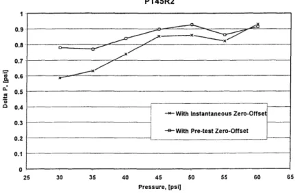
4-2 Non-linearity of Downstream Pressure Transducer PT45R2 with Pressure Level 63
4-3 Non-linearity of Downstream Pressure Transducer PT45R3 with Pressure Level 64
4-4 Non-linearity of Downstream Pressure Transducer PT45R4 with Pressure Level 64
4-5 Non-linearity of Downstream Pressure Transducer PT45R5 with Pressure Level 65
4-6 Non-linearity of Downstream Pressure Transducer PT45R6 with Pressure Level 65
4-7 Non-linearity of Downstream Pressure Transducer PT45R7 with Pressure Level 66
4-8 Non-linearity of Downstream Pressure Transducer PT45R8 with Pressure Level 66
4-9 Correction Curves for Downstream Pressure Transducer PT45R1 ... 67
4-10 Correction Curves for Downstream Pressure Transducer PT45R2 ... 67
4-11 Correction Curves for Downstream Pressure Transducers PT45R3 .... . 68
4-12 Correction Curves for Downstream Pressure Transducers PT45R4 .... . 68
4-13 Correction Curves for Downstream Pressure Transducers PT45R5 .... . 69
4-14 Correction Curves for Downstream Pressure Transducers PT45R6 .... . 69
4-15 Correction Curves for Downstream Pressure Transducers PT45R7 .... . 70
4-16 Correction Curves for Downstream Pressure Transducers PT45R8 .... . 70
5-1 Contour Plot of Adiabatic Efficiency Uncertainty as a Function of ep and 6T 74 5-2 Enthalpy-Entropy Diagram for the Expansion Processes in Turbines . . . . 77
6-1 Inlet Total Temperature of Test ABB011 at Midspan . ... 85
6-2 Exit Total Temperature of Test ABB011 at Midspan . ... 85
6-3 Inlet Total Pressure of Test ABBO11 ... ... 86
6-4 Exit Total Pressure of Test ABB011 . ... . .. 86
6-5 Temperature Ratio of Test ABBO11 ... ... 87
6-6 Pressure Ratio of Test ABB011 ... ... 87
6-7 Adiabatic Efficiency of Test ABB011 ... ... 88
6-8 Rake Efficiency of Test ABB011 ... ... ... 88
6-9 History of Specific Heat Ratio y for C02 in Test ABBO11 . ... 89
6-10 ABB011 Inlet and Exit Points in h-s Diagram ... ... 90
List of Tables
2.1 MIT Blowdown Turbine Scaling ... ... 15
2.2 Various Pressure and Temperature Transducers at MIT BDT . ... 18
3.1 Temperature Probe RTD Bridge Comparison . ... 35
3.2 Naming Convention for Total Temperature Rake Sensors . ... 37
3.3 Specificcations for Rosemount Standard Platinum Resistance thermometer Model 162N ... ... ... 39
3.4 Calibration Results of Upstream and Downstream Rake RTDs . ... 42
3.5 Uncertainty in Total Temperature Measuremnet . ... 50
4.1 Naming Convention for Total Pressure Rake Sensors . ... 59
4.2 Correction Functions for the Downstream Total Pressure Transducers . . . 62
4.3 Uncertainties in the Total Pressure Measurement . ... 62
5.1 Influence Coefficients for Efficiency Uncertainty . ... 73
5.2 Typical Blowdown Test Conditions for Efficiency Uncertainty Study .... 75
5.3 Uncertainties in Adiabatic Efficiency Measurement . ... 75
6.1 Target Test Conditions for ABBO11 ... ... 83
6.2 ABBO11 Inlet and Exit Parameters at Different Time Moments ... . 84
Chapter 1
Introduction
1.1
Motivation
Over the past 40 years the aerodynamic performance of gas turbine engines have been increased enrmously. Although the polytropic efficiencies now are in the low 90% range, research continues aiming at advanced design and better understanding of fluid mechanics which have been made possible through many years of extensive turbine testing. The experiments have been done on engines, rigs and subscale facilities. The cost of real turbine testing has increased tremendously over the years. An uncooled rig test for a large turbine typically costs on the order of $3 million, a cooled test under the same conditions costs about $5 million[7]. The gas turbine engine development program have been greatly affected by the high costs of testing. The only test of some newly designed turbine may be seen in a completely manufactured engine.
In the last few years, however, a new technology based on teansient testing techniques has developed that provides highly accurate, detailed turbine measurements at relatively
low cost[l]. The techniques are based primarily on the realization that the time scale
characteristic of the physical processes within a turbine may be indeed quite short (on the order of hundreds of microseconds). If the test time includes thousands or tens of thousands of characteristic flow time, sufficient for establishing steady state behavior of gas flow, and
provided that instrumentation has fast frequency response, the actual running of the turbine rotor would be quite short (less than a second). Due to the short interval of testing time, the total energy consumption is very, very low. The construction, maintenance costs of the short-duration rig, and the power cost of tests are greatly reduced. The MIT Blowdown Turbine facility (BDT) is such a short-duration test rig.
This work uses the Blowdown Turbine facility at MIT to investigate the aerodynamic performanece of a scaled single stage turbine. A detailed study of advanced instrumentation for short-duration test facility and measurement uncertainty will be presented in next few chapters. Also, the difference of efficiency measurements between steady state test and transient test, and the results of two independent efficiency measurements will be addressed.
1.2
Objective and Approach
From thermodynamics we know that the efficiency of a turbine can be defined as
Wa
r = (1.1)
/Videal
where Wa is actual work produced by the turbine, and /Videal denotes the ideal work of
the turbine in an isentropic expansion. The ideal work can be calculated as
Wideal - rh Cp T 1 - P1 2) (1.2)
where
rh
is the mass flow rate, Cp is the specific heat of gas, T1 and P1 are the totaltemperature and total pressure of gas at the inlet of the turbine, P2 is the total pressure of
gas at the exit, -y is the specific heat ratio.
There are two ways of writing the actual work Wa. First of all it can be written as
Wl = T w (1.3)
where T is the shaft torque delivered by the turbine rotor, and w is the rotor speed (in radian/sec). The other way of defining WV, is through thermodynamic process. In steady
state a turbine runs under adiabatic condition and its work can be written as
Wa = rh Cp (Ti - T2,ad) (1.4)
where T2,ad is the total temperature of gas at the exit of a turbine in an adiabatic process. Following the first definition of the actual work we can abtain the first definition of turbine efficiency as
T (1.5)
This definition of turbine efficiency yields a way of measuring it. This approach is usually called mechanical approach. The necessary quantities we need to measure are mass flow rate r~a, shaft torque T, rotor speed w and aerodynamic parameters at inlet and exit
of the turbine TI, PI and P2. This approach for efficiency measurement has been realized
in MIT BDT. A more detail description of experimental setup, calibrations and results are presented in [18].
If the working gas is ideal and its properties are constant, the process-defined actual work (eq. (1.4)) leads us to the most commonly used definition of adiabatic turbine efficiency. It can be written as[9]
1-7 ad = 1 (1.6) where
T2
7 - (1.7)T,
P2
SP2 = (1.8) P1Equation (1.6) tells us that in order to make efficiency measurement it is enough to know the aerodynamic parameters at inlet and exit of a turbine. So measuring inlet and exit total temperatures and total pressures would give the answer for the adiabatic efficiency of a
turbine. This approach is the thermodynamic approach of turbine efficiency measurement, and is also utilized in the MIT BDT. This thesis is mainly focused on this method.
The above two approaches have been applied in the MIT Blowdown Turbine facility to investigate the performance of a single stage turbine. Both methods demonstrated very close results and provided a deep examination of the nature of short-duration turbine testing. A comparison of the two independent measurements and an analysis of influence of
non-adiabatic effects on efficiency measurement are given in chapter 5 and chapter 6.
1.3
Thesis Outline
The remainder of the thesis is organized into the following chapters.
Chapter 2 describes the Blowdown Turbine facility. A brief description of the operation of the test rig is presented. The accuracy requirement for temperature measurement, tem-perature sensor development, design and calibration of the total temtem-perature probes and assessment of sensor performance are covered in chapter 3. Chapter 4 deals with pressure measurement. The total pressure probe design and calibration are shown. The uncertainty in pressure measurement is assessed. This is followed by a chapter on efficiency calculation. The difference of efficiency measurements between short-duration test and steady state test is also analyzed in this chapter. The experimental results are presented in chapter 6. A final summary and conclusion are provided in chapter 7. Suggestions for future work are also discussed.
Chapter 2
Experimental Facility
This chapter describes the experimental facility used for aerodynamic performance mea-surements of a single stage turbine. A brief description of the configuration and operation of the facility during a typical run, instrumentation for the performance measuremnets and the data acquisition systems are presented.
2.1
The MIT Blowdown Turbine Facility
The experiements for the investigation of aerodynamic performance of a single stage turbine were conducted on the MIT Blowdown Turbine (BDT) test rig. The Non-dimensionalized equations of continuity, motion and energy show that it is the ratio of forces, fluxes and states that determine the flow field. Therefore, only the non-dimensional parameters and boundary conditions, but not the actual running conditions, need to be matched for the simulation of engine operation. These parameters are Reynolds number, Prandtl number, Mach number, Rossby number, ratio of specific heats, corrected speed, corrected weight flow and gas-to-metal temperature ratio. The blowdown turbine is a short-duration test facility which rigorously simulates the operational environment of actual gas turbine engines by matching these non-dimensional parameters. This section serves only to briefly describe the configuration of the MIT Blowdown Turbine. Details of the facility design and tunnel operation can be found in references [5, 4]. Table 2.1 provides the scaling of the BDT facility
I-Table 2.1: MIT Blowdown Turbine Scaling
compared to a full scale gas turbine.
An mixture of Argon and C02 is used as the test gas. The desired
7
sets the mixtureratio. Using the mixed gases instead of air has several advantages. The Argon - C02
mixture has larger density and reduces pressure level to achieve Reynolds number similarity. With the lower pressure level the power generated by the turbine is decreased and this makes the experimental facility safer and easier to manage. Also, the lareger molecular weight of the mixed gases reduces the speed of sound which decreases the rotor speed for tip Mach number similarity. The slower rotor speed asks for lesser requirement on the bandwidth of high frequency instruments. More importantly, the slower rotor speed reduces the stress level in the blades, disks, seals and other rotating parts.
A schematic of the blowdown turbine facility is shown in Figure 2-1. The blowdown turbine test facility has four major components: supply tank, fast acting valve, test section and dump tank. The supply tank has an oil jacket which serves to heat the gas mixture before a test. The fast acting valve separates the test section and the supply tank. The test section consists of a forward frame, a circumferential boundary layer bleed, 44 nozzle
Parameters Full Scale Engine MIT BDT
Working Fliud Air Argon - CO2
Ratio of Specific Heats, y 1.28 1.28
Mean Metal Temperature 1100 K (15210F) 300 K (810F)
Metal/Gas Temp. Ratio 0.647 0.647
Inlet Total Temperature 1700 K (26000F) 464 K (3760F)
NGV Chord (midspan) 0.146 m 0.0365 m
Reynolds Number 5.6 x 10⁶ 5.6 x 10⁶
Inlet Total Pressure 15 atm (224 psia) 7 atm (105 psia)
Exit Total Pressure 7.43 atm (111 psia) 3.47 atm (52 psia)
Exit Total Temperature 1470 K (21870F) 401 K (2620F)
Prandtl Number 0.928 0.742
Design Rotor Speed 3600 rpm 5954 rpm
Design Mass Flow 312 kg/s 23.3 kg/s
Turbine Power Output 91.13 MW 1.26 MW
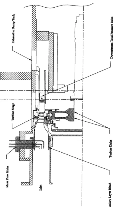
guide vanes (NGV), a rotor with 88 blades, a downstream translator serving as inner wall of the flow path downstream of the rotor, a throttle plate which sets the exit conditions and turbine pressure ratio, an eddy current brake and a 10 hp motor mounted on the shaft of the turbine rotor. Cross-sectional view of the test section and the flow path is illustrated in Figure 2-2. There are nine instrumentation window ports for access to the flow field. Three circular ports equally spaced 1200 apart are located upstream of the NGV, serving as access window for total temperature and total pressure rakes. Another three circular ports upstream of the NGV were newly made for mass flow meters. They are also 120' apart, but 20' away from the first group of windows. In addition, three 13 cm wide rectangular windows are equally spaced around the outer wall of the test section and extend from upstream of the NGV's to 11 cm downstream of the rotor.
2.2
Operation of MIT Blowdown Turbine
A brief description of the operation of the BDT during a typical test is given in this section. First, the tunnel is evacuated by an external vacuum system. The supply tank is heated up to the desired temperature by circulating heating oil through the oil jacket of the tank. Once the temperature is reached, the fast acting valve (also referred as main valve) is closed. Then the test gas mixture is loaded into the supply tank to the required level. The translator, eddy current brake and data acquisition systems are set in standby-mode. The rotor is spun up in vacuum by a drive motor to above the desired speed. Then the drive motor is shut off, and the rotor slows down because of the bearing friction. When the rotor speed matches the preset value, firing circuitry is triggered. With the trigger, the following actions are taken: the fast acting valve is open, the data acquisition systems start to take data, the eddy current brake is energized. After a 200 millisecond initial transient of the blowdown, the downstrean throttle plate is choked, and the blowdown process enters a quasi-steady state which lasts for about 300 milliseconds. During this time period, the turbine corrected speed and pressure ratio stay virtually constant to better than 1%. The flow in the tunnel lasts approximately one second until the downstream throttle late is unchoked. The data
acquisition systems continue to take data for ten minutes to monitor tunnel conditions and to provide calibration data for the intruments.
2.3
Instrumentation and Data Acquisition
2.3.1 Instrumentation of the Blowdown Turbine Facility
The MIT Blowdown Turbine is a sub-scaled turbine testing facility. Due to the testing advantages mentioned in ealier sections the rig is instrumented with many advanced force and flow sensors.
A torque meter was designed to survey the torque history. The eddy current brake which is used to absorb the energy generated by the turbine now is floated on two bearings. Two loadcells are mounted on a plate which holds the eddy current brake coils. The torque delivered by the rotor shaft is transmitted through the brake to the loadcells. The details of the design and operation of the torque meter can be found in reference [18].
Upstream of the NGV there are five probe rakes. A total temperature probe rake with 6 heads is located right ahead of the inlet of the NGVs. This rake has a reference block built in the rake body. The probe heads have 0.0005 inch diameter type K thermocouples which have sufficient response time to see the compressional heating of the start-up transient of the blowdown tests. A detailed description of the design and calibration and an uncertainty analysis are the subject of chapter 3. A 6-head impact total pressure probe rake is mounted at the same axial location but 120' apart from the upstream total temperature probe. The total temperature and total pressure rakes monitor the radial variation of the flow param-eters and also provide spatially averaged values of the upstream stagnation paramparam-eters. A group of three new mass flow probes is placed 1200 apart from each other. This mass flow probe measures the total temperature, total pressure and dynamic head of the gas at the same location and at the same time. With measured dynamic pressure and total pressure, total Mach number can be inferred, and with know geometry the mass flow rate can be calculated. Additional description of this probe can be found in [18].
Downstream of the rotor there are three probe rakes mounted on the dowstream trans-__
Table 2.2: Various Pressure and Temperature Transducers at MIT BDT
Name Type Location Sensor(s) Range Comments
PTOA Total Supply Kulite 0-150psig Redundat
PTOB Pressure Tank XTE-190
P45A Wall Static Downstream Kulite 0-150psig Flush Mounted
Pressure Rotor Exit XTE-190
P45HUB Wall Static On Exit Kulite 0-100psig On Inner
Pressure Translator XCQ-063 Annulus Wall
PDMP Total Pressure Dump Tank Kulite 0-50psig
XTE-190
TTO-U Total Supply Tank T/C, type K 270-550 K For Initial
TTO-M Temperature Temperature,
TTO-L I I I I 1 3 locations
lator which is essentially the inner annulus wall for the flow path. The translator is motor-driven and computer-controlled to rotate 3200 during a test (2400 within 300 msec valid test time). Three canisters are mounted on the translator. These canisters are able to hold three probes which are supposed to be interchangeable to match the wiring diagram. The wires coming out of the translator are copper wires. The design and operation of the downstream translator can be found in [20]. Two total temperature rakes are mounted on the translator. One has five heads and the other has four. The design of the downstream total temperature rakes are similar to the upstream rake, and the details of their calibra-tion and uncertainty are given in chapter 3. A low-frequency total pressure rake is mounted beside the temperature rakes. The low-frequency pressure rake has eight impact heads to resolve the radial variation of the flow at the exit of the rotor. The pressure transducers are mounted in the rake body to avoid the drift of the transducers due to the temperature variation [10].
Other temperature and pressure sensors, listed in table 2.2 [11], are also employed in the facility to measure the temperature and pressure in the supply tank, test section and dump tank.
2.3.2 Data Acquisition
Though a single blowdown test lasts only for about 1 second, enormous amout of test data is sampled and taken into computer memories. For sampling purpose three data acquisition systems are employed in the BDT. These systems are described below.
1. A MIT custom-designed 12-bit DAS A/D consisting of 45 high speed channels and
eight 16-channel multiplexers is used for high and low frequency pressure transducers. This system was also used for heat flux measurements in previous research projects in the BDT. The highest sampling frequency on the high speed channels is 200 kHz. The whole A/D system is run from a DEC MicroVAX II computer. During the test, data is stored into a 32 Meg RAM unit, and after the test it is moved to an internal hard drive. The details regarding this A/D system can be found in [5] and [4].
2. ADTEK Corp. model AD-830 8-channel 12-bit A/D with a maximum sampling frequency of 333 kHz per channel is also used for high frequency pressure transducers and heat flux gages. Four of these A/D boards are installed in a ALR Revolution II computer. The clocking of the boards is synchronized to the MIT BDT A/D system.
3. Analogic model HSDAS-16 16-bit A/D card with AMUX-64-16 multiplexer was used for thermocouple sensors, reference junction RTDs, mass flow meter and torque meter. The sampling frequency of this system was set as the following:
0 - 1000 msec: 3.03 kHz
1000msec - 10 min: 1Hz
The sampling frequency of the first two systems is given below.
0 - 250 msec: 50 kHz 250 - 550 msec: 200 kHz 550 - 1200 msec: 50 kHz 1200 msec - 10 min: 50 Hz
_
_
_
X_
P
__I_
1 Meter
Figure 2-1: Schematic of the MIT Blowdown Turbine Facility
20
_ I __
4!
I
Figure 2-2: MIT Blowdown Turbine Facility Flow Path
Figure 2-2: MIT Blowdown Turbine Facility Flow Path
Chapter 3
Total Temperature Measurement
3.1
Introduction
The goal of this work is to investigate aerodynamic performance of a turbine by using the thermodynamic approach discussed in section 1.2. This approach requires determination of total temperature and total pressure upstream and downstream of the turbine stage. The technology for temperature measurement in conventiotal steady state testing facilities is well developed. As mentioned in section 1.1, the blowdown test is a transient process which rigorously simulates the characteristics of fluid dynamics and heat transfer in turbo-machinery. The real-time knowledge of flow parameters such as temperature and pressure is extremely important to the measurements made in blowdown environment. High accuracy, fast response and low cost are the primary requiremnets for the temperature probe design. In previous research projects conducted in the MIT BDT different methods and designs have been developed to measure total temperature. Different thermocouples, different thermal insulations for preventing heat losses and different geometric configurations were studied by Cattafesta. In [3] Sujudi studied two other methods of reducing the error caused by heat losses. One was to measure the base temperature of the thermocouple probe stem. By measuring the temperature difference between the base and the tip one could compensate the heat losses. The other approach was to heat the probe up to certain temperature prior
to a blowdown test. By doing this one might reach the response time required for blow-down type experiment. Besides, Sujudi gave a very good analytical model to theoretically compensate the error induced by heat conduction and radiation. All the efforts made for temperature measurement in the BDT did not bring satisfactory results for aerodynamic performance study.
In this work a new concept of impact total temperature probe was developed. This chapter will first give a brief introduction to the fundamental laws of thermocouple technol-ogy. The requirements for total temperature probe in blowdown test envionment is again emphasized. The new probe configuration and a heat transfer model are developed. Also the construction of the probe itself and reference junction is described. Static calibration of the thermocouples and the reference junction will be addressed. Finally, uncertainties involved in the total temperature measurements will be estimated.
3.2
Requirements for Total Temperature Probe in
Blow-down Environment
Due to the nature of transient testing there is a crucial distiction between total temperature measurements in BDT and in a conventional steady state facility. In steady state test facility the inlet and exit temperatures of a turbine are constant with time, and the test time is very long compared to the frequency response of temperature probes. But in a blowdown type experimental facility this is not the case since the test time is very short. Therefore, the time response is a great concern even for quasi-steady period of a blowdown test. The temperature probe initially sits in the tunnel under room temperature. After 30 msec the main valve opens. The following 70 msec establishes quasi-steady flow. From 200 msec to 500 msec the corrected speed, corrected weight flow and other flow parameters are held constant. So the temperature probe is supposed to heat up to gas temperature before the quasi- steady period starts and is required to be fast responsive so that it can monitor the real-time change of flow temperature.
As will be discussed in chapter 5, the uncertainty of temperature measurement has a
great play in determination of efficiency measurement uncertainty. The influence coefficient due to temperature measurement error weighs approximately three times more than that due to pressure measurement error. The goal of this work is to measure total temperature with less than 0.2 K uncertainty.
Also the total temperature probe should not be sensitive to flow angle. For upstream total temperature probe this is not a big problem, because the inlet flow contour of the test section and the boundary layer bleed make the inlet flow uniform. Downstream of the rotor the total temperature probe is required to be insensitive to the wake mixing and swirling flow.
3.3
Basic Theory of Thermocouple Technology
It was Seebeck who discovered the existence of thermoelectric currents while observing electromagnetic effects associated with bismuth-copper and bismuth- antimony circuits. His experiments showed that, when the junctions of two dissimilar metals forming a closed circuits are exposed to different temperatures, a net thermal electromotive force is generated which induces a continuous electric current. Today thermocouple technology is extensively used in measuring temperature and other heat phenomena. The detailed theory of thermo-couple can be found in [2] and other literature. Here we present three fundamental laws of thermoelectric circuits which will be frequently referred in later sections.
(1)A thermoelectric current cannot be sustained in a circuit of a single homogeneous
material, however varying in cross section, by the application of heat alone.
In other words, two different materials are required for any thermocouple circuit. (2) The algebraic sum of the thermoelectromotive forces in a circuit composed of any number of dissimilar materials is zero if all of the circuit is at a uniform temperature.
An obvious consequence of this law is that a third homogeneous material always can be added in a circuit with no effect on the net emf of the circuit so long as its extremities are at the same temperature.
(3) If two dissimilar homogeneous metals produce a thermal emf of El, when the junctions
are at temperatures T1 and T2, and a thermal ernf of E2, when the junctions are at T2 and
T3, the emf generated when the junctions are at T1 and T3 will be E1 + E2.
Two consequences can be induced from this law. First, a thermocouple calibrated for a given reference temperature can be used with any other reference temperature through the use of a suitable correction. Second, extension wires, having the same thermoelectric characteristics as those of the thermocouple wires, can be introduced in the thermocouple circuit without affecting the net emf of the thermocouple.
The standard thermocouple tables are made for 00C reference temperature. In these tables O0C corresponds to 0 volts EMF. In most cases, the reference temperature cannot
be set to 000C, and a reference junction is usually used. Following the second and third
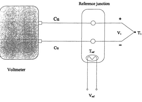
laws above, one can arrive at a simple way of measuring temperature. Figure 3-1 shows the diagram of thermocouple circuit with an external reference junction. A detailed description of how to derive this circuit can be found in [16]. In the diagram, thermocouple junction
generates EMF caused by the difference between the source temperature T1 and the
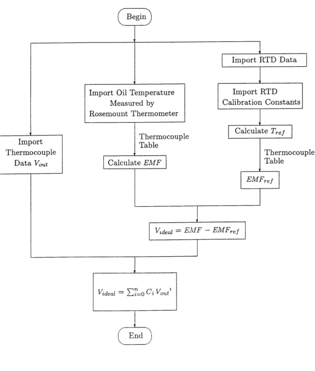
tem-perature of reference junction Tref. An external voltmeter reads this EMF. A reference thermometer provides us the absolute temperature (in reference to 0°C) of the reference junction. The reference temperature Tref can be converted to voltage Vref according to the thermocouple table. Adding Vref to the EMF measured by voltmeter, we obtain the absolute EMF, and again by using the thermocouple table we find the absolute source tem-perature. This method gives us a very flexible way of measuring temperature, because the reference junction can be set to any convenient temperature as long as the reference ther-mometer is properly calibrated. An important point should be made here: the temperature within the reference junction should be kept uniform at all time during a test. If a filter and an amplifier are used for better signal conditioning. not only the reference thermometer but also the thermocouple needs to be calibrated.
Reference junction
Voltmeter
Figure 3-1: Thermocouple Circuit with External Reference Junction
3.4
Total Temperature Probe Design
3.4.1 Probe Head Design and Model
In the MIT BDT, type K thermocouple has been chosen as major temperature measuring tool for many years because of its stability and linearity. Prior to this work, a few total temperature probes had been designed, but none of them turned out satisfactory. The most recent design was done by Sujudi. In [3] the total dynamic error of temperature measurement was estimated as 5 to 9 K, and the static error was 0.1 K - 0.2 K. The error sources were conduction of the wire and supporting ceramic stem, radiation, recovery and calibration. The response lag was also a major contributor of error.
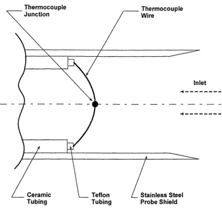
In this work a new design of total temperature probe has been developed. To reduce the response lag a 0.0005 inch diameter thermocouple is used. As shown in Figure 3-2 the thermocouple junction bead is located in the middle of the probe. The thermocouple wire is hung across the probe inner diameter. Shielded by small teflon tubing, the wires run
Thermocouple
Junction ThermocoupleWire
Inlet -- - --- .4---Ceramic \L_ Teflon Tubing Tubing Stainless Steel Probe Shield
Figure 3-2: Schematic of Thermocouple Probe Head Design (Not to Scale)
down to further connection through a pair of ceramic tubes. In previous designs, only the thermocouple junction is heated and almost no wire length was exposed to the test gas. The wires worked as a main conduction error source. In the new design, significant wire length is exposed to the test gas. The gas passing through the probe, heats not only the thermocouple junction but also the wires, and this leads to great reduction of conduction and radiation losses.
Conventionally, first-order lumped capacitance method is used to model thermocouples. The essence of this method is the assumption that the temperature of the solid is spatially uniform at any instant during a transient process. This assumption implies that temperature gradients within the solid are negligible. In a short-duration blowdown test process the transient phenomena play a critical role in temperature measurement. We need to ask:
T(r,O)=1.
Tm, h
I I I
I I I
Figure 3-3: Infinite Cylinder with Initial Uniform Temperature Subjected to Sudden Convection Conditions
How long does it take for the center line of thermocouple wire to reach the actual test gas temperature (or say 99% of the gas temperature)?
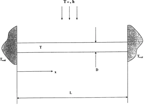
The thermocouple wire length which is hung across the probe and exposed to the gas is much larger than the wire diameter. This allows us to use the infinite cylinder model to calculate the transient conduction of the wire. Figure 3-3 shows the simplified model of the wire cross-section. For an infinite cylinder only one spatial coordinate is needed to describe the internal temperature distribution. Heat equation can be reduced to
a2T 1 aT
Or- 2 a Ot (3.1)
Or2
cv t
To solve equation 3.1 it is necessary to specify an initial condition and two boundary conditions. The initial condition is
T(r, 0) = T, (3.2)
and the boundary conditions are
OT
T =0 (3.3)
Or r=O
and
- k - = h [T(ro, t) - T.] (3.4)
r r=ro
where h is the convection heat transfer coefficient, and k is thermal conductivity of the thermocouple wire.
Equation 3.2 presumes a uniform temperature distribution within the infinite cylinder
at time t = 0; Equation 3.3 defines the symmetry requirement and equation 3.4 describes
the surface condition experienced for time t > 0.
To generalize the solution for equation 3.1 a dimensionless form of the dependent variable can be defined as
" T - Too T-T (35)(3.5)
Ti - Too
A dimensionless coordinate can be defined as
r* = r (3.6)
ro
Well-known Fourier number can represent dimensionless time as
t* - t Fo (3.7)
then the heat equation becomes
a2,9* 01"
&2- =(3.8)
Or
* 2 - aFoand the initial and boundary conditions become
id*(r*, 0) = 1 (3.9)
=I 0 (3.10) ar* r*=O and = 1 = -i - 9*(1, t*) (3.11) r*" r*
where the Biot number is Bi hr
The exact solution in dimensionless form for equaiton 3.8 can be found in [8]. The
dimensionless temperature is 00 * =
S
exp(-Fo) . Jo(nr*) (3.12) n=l where 2 J1 ((n) n J2( + J() (3.13)and the discrete values of Cn are positive roots of the transcendental equation
(n
) Bi
=
(3.14)
Jo(Cn)
J1 and Jo are Bessel functions of the first kind. In our case, Biot number can be
determined from the wire geometry and typical flow parameters. Solving equation 3.14 we
can find discrete values of Cn and (n. Substituting these Cn and (n into equation 3.12
we can determine non-dimensionalized time Fo then convert it to real time. The final solution for the transient conduction problem in an infinite-long thermocouple wire gives us the answer asked early in this section: It takes 26 miliseconds for the center line of type K thermocouple wire to heat up to 99% of the ambient gas temperature at upstream conditions, and 10 miliseconds at downstream conditions. This calculation shows that this tepmerature probe design provides a very fast response. During the first 26 milisecond of the blowdown startup transient, the thermocouple wire would heat from room temperature
up to the test gas temperature.
In the MIT Blowdown Turbine test rig a phenomenon known as compressional heating
has been observed at the early stage of startup transient [10]. The high pressure in the
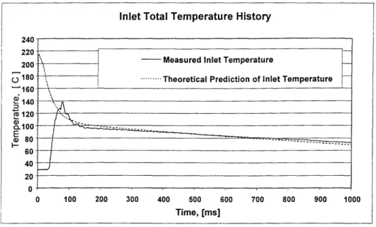
supply tank coupled with the initial vacuum in the test section has the effect of compress-ing the gas, and therefore heatcompress-ing it. Compressional heatcompress-ing is a transient phenomenon and lasts only a short time until the pressure equalizes in the tunnel. In the total tem-perature probe development process not all probe could see this phenomenon. Cattafesta's preheated probe was the first temperature probe which could observe it. So whether a new probe can see compressional heating in a blowdown test becomes an experimental criterion for probe response qualification. The new total temperature probe can easily detect this rather interesting effect. Figure 3-4 shows an inlet total tempeture history of a blowdown test observed by the new-concept total temperature probe. A clear spike can be seen at around 75 msec. In figure 3-4 the dashed line represents a theoretical prediction of the inlet total temperature. The assumptions of the theoretical model are isentropic expansion and constant y. Practically, it takes about 34 ms for the temperature probe to see the hot gas because of the main valve open time and the distance from the valve to the probe, and about 26 ms for the center line of the thermocouple wire to reach the gas temperature. Then due to the transient conduction effect, the themocouple wire temperature overshoots the gas temeperature. Afterwards, the wire quickly cools down to the gas temperature level and tracks the inlet gas temperature during the blowdown test.
3.4.2 Reference Junction Design
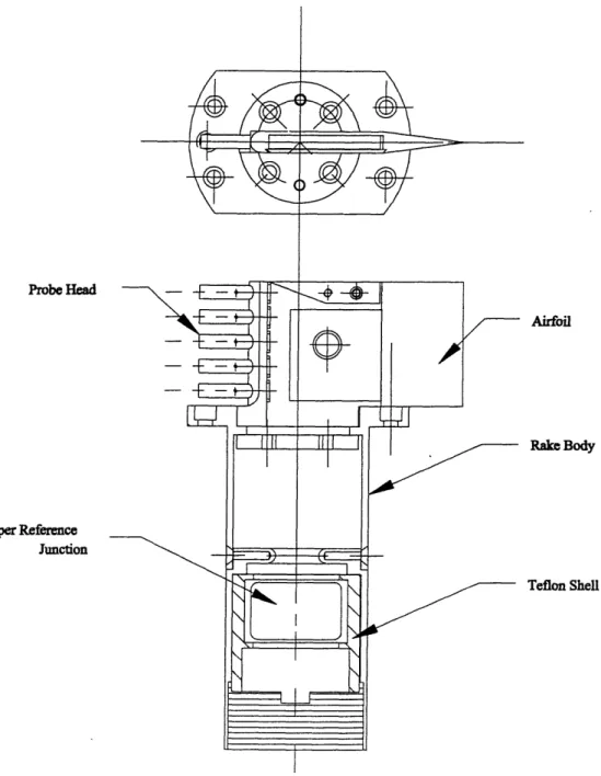
As mentioned in section 3.3 a reference junction is needed for measuring temperature (see Figure 3-1). The temperature within the reference junction should be uniform during a test. Cylindrical shape copper blocks were chosen as reference junctions for upstream and downstream temperature rakes. These copper cylinders are located inside the probe rake bodies and shielded by teflon shells which insulate the copper blocks from effective thermal contact. The temperature of reference junction is measured via resistance temperature
__ _*__._ _ ~
Inlet Total Temperature History
Figure 3-4: Compressional Heating in a Blowdown Test Seen by the New Temperature Probe
devices(RTDs).
In previous total temperature probe designs, 50-ohm nickel-film RTDs mounted on cop-per block surface were used to monitor reference temcop-perature. The uncertainty of this type
of RTD was good to 0.1 - 0.2 K. Our design goal is to eliminate the errors along the
temperature measurement chain down to 0.2 K. Apparently this type of RTD is not suit-able for our aim. A new RTD design was suggested. This design is essentially a six-wire bridge circuit. Figure 3-5 shows two circuit diagrams of this type of bridge. The first circuit has only one RTD while the second has two on its opposite legs. RTD can be viewed as a resistor which changes its resistance with temperature. Mathematically it can be written as
RTD = R2 +
where SR is the resistance which changes with temperature, and R2 is RTD's basic
resistance.
0 100 200 300 400 500 600 700 800 900 1000
Time, [ms]
+ Excitation + Sensing
- Sensing - Sensing
(1) (2)
Figure 3-5: Schematic of Six-wire Wheatston Bridge RTD Circuitries
The voltage drop across the bridge is a function of RTD's resistance, i.e. a function of temperature. A little algebra would help find the relation between the voltage drop AV and resistance change SR. For circuit 1,
R - R 2 R2 SR AV = V 1 2 (3.15) (Ri + R2)(R1 + R2 + 6R) For circuit 2, R1 - R2 - R AV = V (3.16) RI + R2 + 6R
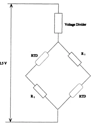
If compare equations 3.15 and 3.16, one can see that AV is more sensitive to SR in circuit 2 than in circuit 1. Therefore, circuit 2 was chosen for further study. When the bridge is excited by external voltage, RTDs as resistors dissipate power and convert it into heat. So there is difference between the temperature measured by RTDs and the actual temperature of copper block. To reduce the heat generation a voltage divider is applied. Figure 3-6
III
shows the circuit diagram. Now a question rises. What values of resistors and RTDs should be selected to decrease the temperature difference between the RTD and reference juncion
down to minimum.
Voltage Divide
RTD R
2.5 V
Figure 3-6: Schematic of Six-wire Wheatston Bridge RTD Circuitry with Voltage Divider
An one-dimensional conduction model is assumed. The heat rate between an RTD and copper block is
dT qz =
-kA--dx (3.17)
V'
In our case qx is the power generated by RTD which is R , k is the thermal
conductiv-ity of adhesive - polypropylene which equals 0.17.n , A is the contact area of RTD. dT is
the temperature difference AT across the adhesive, and dx is the thickness of the adhesive.
Table 3.1: Temperature Probe RTD Bridge Comparison
Bridge Voltage RTD Constant Power AT
Circuit Divider Resistor Dissipation per RTD
[ohm] [ohm] [ohm] [Watt] [K]
Circuit 1 1000 100 100 1.29 10- 4 0.009
Circuit 2 500 50 50 2.58 10- 4 0.019
Circuit 3 1000 1000 1000 3.9 10- 4 0.028
The lowest excitation voltage we can get from the ampplifier is 2.5 volts. To decrease the voltage across the bridge, a voltage divider is used. Three bridge circuits with different voltage dividers, RTDs and constant-resistors are compared with each other. Table 3.4.2 summarizes the resluts of calculation.
Obviously, circuit 1 with 1000 ohm voltage divider and 100 ohm RTDs, 100 ohm constant resistors is the best choice, because the temperature difference between RTD and reference junction caused by self-heating is negligibly small.
For upstream and downstream total temperature rakes, OMEGA model F3102 100 ohm
RTD (a = 0.00391 ohms/ohm/'C, American standard curve) was chosen to measure the
temperature of reference junction. Micro Measurements hermetic precision resistors
H-1000-01 and H-100-H-1000-01 (temperature coefficienct = ±1 ppm/oC) were used as voltage divider and
bridge constant resistors for upstream temperature rake. Due to geometric constraints, Micro Measurements plastic precision resistors S-1000-01 and S-100-01 (temperature
coef-ficienct = ±1 ppm/'C), which are smaller than hermetic resistors, were selected as voltage
divider and constant resistors for downstream temperature rake. As will be shown in section 3.5.2, these RTDs are very accurate and stable.
3.4.3 Upstream and Downstream Total Temperature Rakes
Upstream total temperature rake has six vented heads. In every head an OMEGA 0.0005 in diameter type K thermocouple is hung across the inner diameter of the head. Two ceramic
tubings are glued by epoxy 276 which can stand high temperature up to 2600C. These
two ceramic tubings are set apart as far as the inner diameter of the stainless steel probe head. The ceramic assembly is glued into the probe head and provides structural support for the thermocouple wires. The thermocouple wires are shielded by small teflon tubings which run through the ceramic tubings and come out of the head bottom. These six vented probe heads are glued into an airfoil which reduces the disturbance to the flow. From each head two thermocouple wires come out and are soldered onto bigger type K thermocouple wires on copper solder pads. The solder pads are glued on a rubber insulation. This rubber insulation reduces the heat transfer between the solder pads and the airfoil wall down to almost zero, which guarantees the uniform temperature of the solder pads during a test (see the second law of thermocouple theory in section 3.3). Coming out of the airfoil the bigger thermocouple wires go into the rake body and are soldered on the reference junction. These stronger thermocouple wires are made 12 inches long to provide calibration convenience. The reference junction is a cylindrical copper block. Two six-wire RTD bridges are also glued on the copper block to measure its temperature uniformity. This copper block is shielded by a pair of teflon shell which works as a thermal insulation. Within the teflon shells the copper block maintains a uniform temperature during a blowdown test which virtually lasts for a second. All the thermocouple wires are soldered onto copper wires for further connection. A Bendix connector sits at the bottom of the rake and provides electric connection to signal conditioner.
Two downstream total temperature rakes were manufactured in the MIT Gas Turbine Laboratory. One has five heads and the other has four. The nine downstream tempera-ture heads radially cover the whole flow path downstream of the rotor. Structurally the downstream rakes are the same as the upstream one. As mentioned in section 2.3.1, the downstream rakes are installed in the canisters of the downstream translator. The size of the canister puts geometric constraints on the downstream temperature rakes. The size of the reference junction is smaller than that of the upstream rake. 12-inch long extention thermocouple wires are kept to provide the possibility of separating the thermocouple heads and the reference junction during the calibration. Figure 3-7 shows an assembly drawing of the five-head rake.
Table 3.2: Naming Convention for Total Temperature Rake Sensors
Sensor Name Location
TTR101-x1 Upstream of NGV, stationary
TTR103-x Downstream of Rotor, 5-Head, translating
TTR104-x Downstream of Rotor, 4-head, translating
The naming convention for the total temperature rake sensors is summarized in table 3.2.
3.4.4 Signal Conditioning
Signals coming out of total temperature rakes are filtered and amplified by Analog Devices signal conditioners model 2B31L. After amplification the signals are fed into multiplexer A/D system, which is described in chapter 2. This type of signal conditioner module has
small offset drift with temperature and time (0.6 MV/'C and 3 1V/month from
specifica-tions), and low gain nonlinearity (0.0025% max from specifications). Experiments indicate offset variation of less than 0.0006 mV (correponding to 0.0010C at gain of 1000) during a typical day. The conditioner module provides an adjustable-gain amplifier, a three-pole low pass filter, and also an adjustable transducer excitation, which is used to provide current and voltage excitation for the reference juunction RTDs.
Signals from the upstream temperature rake (TTR101) and five-head downstream tem-perature rake (TTR103) are amplified at a gain of 415, while the signals from four-head downstream temperature rake (TTR104) are amplified at a gain of 800. All thermocouple signals are low-pass filtered at 500 Hz. Signals from the reference junction RTDs of the upstream rake are amplified at a gain of about 380, signals from the RTDs of the five-head temperature rake are amplified at gains of 368 and 386. while those of four-head downstream temperature rake at gains of 394 and 430. All RTD signals are low-passed filtered at 2 Hz.
The 16-bit A/D operates at ±10 V range and has a resolution of 0.3 mV. Thus it
1,"x" refers to the sensor number, 1 being at the rake tip.
provides temperature resolution of 0.02, 0.02, 0.01, and 0.0020C for the upstream, five-head downstream thermocouple sensors, four-five-head downstream thermocouple sensors and
all reference junciton RTDs, respectively.
High frequency signal noise is about ±1 mV for all sensors, corresponding to ±0.0600C for the upstream and five-head downstream thermocouple sensors, ±0.03°C for the four-head downstream thermocouple sensors, ±0.006'C for all reference junction RTDs.
3.5
Static Calibration of Total Temperature Probe
As mentioned in section 3.3, the RTDs of the reference junction and thermocouple sensors must be calibrated. This section describes the equipment for calibration and the methods for RTD calibration and thermocouple calibration. Calibration results are given at the end of the section.
3.5.1 Calibration Equipment
Temperature calibration is usually conducted in a medium which is thermally conductive and electrically non-conductive. In the MIT Gas Turbine Laboratory Dow Corning 210H high temperature heat transfer silicon fluid was chosen as the calibration medium for RTD and thermocouple calibration. The silicon oil is contained in a 12-inch diameter by 10-inch deep aluminum pot whose side and bottom are covered by an electric heating jacket and insulation. The top portion of the pot is open for access of instruments. Heating can also be provided through an external Haake B81 heater unit. The calibration pot and the heater are connected through two silicon rubber hoses. The calibration fluid can be circulated via these two hoses by a built-in pump in the Haake heater. The Haake heater also has provisions for cooling the oil bath. This is done by connecting the Haake's heat-exchanger tubes, through two teflon tubings, to city water supply. If calibration has to be done below room temperature, the heat- exchanger can be connected to other cooling source, e.g. water-ice mixture. For heating purpose, both oil pot heater and Haake heater are turned on to provide maximum heat. After calibration data logging begins, both the
Table 3.3: Specificcations for Rosemount Standard Platinum Resistance thermometer Model 162N
Temperature Range -200 to 4000C
Stability 0.100C/year
Self-Heating 28 m W/OC
Time Constant 1.0 sec.
Max. Calibration Uncertainty 0.02500C
(below 2000C )
heaters are turned off, with the circulating pump of Haake heater still on to provide cooling. To maintain a uniform oil bath temperature, a pneumatic stirrer is installed into the oil pot. The stirrer mixes the calibration oil to reduce undesired temperature gradients within the oil bath. This calibration equipment was used for previous research projects and the temperature uniformity of the oil bath was proved to be well within 0.10C for a temperature range from 15'C to 50'C [3]. At higher temperatures, the silicon fluid becomes less viscous, helping mixing. Therefore, the temperature uniformity is expected to increase at higher temperatures.
The oil bath temperature is measured with a NIST-traceable Rosemount Standard Plat-inum Resistance Thermometre model 162N, whose specifications is given in table 3.5.1[19]. The resistance of the Rosemount thermometer is measured by a Fluke 8520A digital mul-timeter. This multimeter can be operated remotely via an integral IEEE-488 interface, allowing triggering from data acquisition computer.
A data-acquisition program, named DVM, is run on a DELL 486D/50 computer. The program reads and records the voltage output of each RTD and thermocouple amplifier through the A/D and the resistance of the Rosemount thermometer through the Fluke digital multimeter. The program displays the temperature measured by the Rosemount platinum thermometer, allowing user to monitor the bath temperature from the screen. The signal sampling averaging rate and data logging interval can be specified at the start of the program. For the RTD and thermocouple calibrations the signal sampling averaging rate is set to be 1024, and the data logging interval is 5 second per data point.
3.5.2 Calibration of Reference Junction RTDs
Upstream temperature rake TTR101 and downstream temperature rakes TTR103 and TTR104 are connected to three signal conditioner. Each signal conditioner has 12 2B31L cards. The last two amplifier cards, i.e. cards No.11 and No.12 are used for the two RTD bridges in each temperature rake. The maximum output range of each card is ±10 volts. During a blowdown test the reference junctions are usually at room temperature, which is about 250C in winter and 30'C in summer. Thus all RTDs are calibrated from room temperature to 500C. To maximize the resolution of the amplifiers, i.e. maximize volts
per OC, two test bridges were made. One simulates 000C and the other simulates 500C.
These two bridges were plugged into the input port of each RTD amplifier successively, and the amplifiers were adjusted to give maximum voltage reading according to the known temperature inputs which actually are fixed bridges.
At first, the following calibration method was applied to upstream and downstream RTDs. During a calibration test the copper block was placed close to the Rosemount plat-inum resistance thermometer. The Haake heater provided heat to the calibration bath. The bath temperature was monitored through DVM program on the screen. After the bath temperature overshot 50'C by a few degree, the Haake heater was turned off, but the circulation pump was left on. The oil then started to cool down. When the temperature dropped down to 500C, the DVM program was manually initiated to start logging data. The bath cooled down because of the convection with air, radiation and mainly the cooling circulation controlled by Haake heater. Data logging stopped automatically when the spec-ified number of data to be taken was reached, or it can be stopped manually at any time during a calibration test. When data logging stopped, DVM sorted the data and stored the data from RTDs and from the Rosemount thermometer in separate files. This calibration method provided the temperature history of RTDs, which is essentially the oil bath tem-perature history, and the voltage output history of RTDs with time. These two groups of data were supposed to track each other at any time moment. Program RTD_CAL reduced the calibration data. It showed an exponential drop of the bath temperature and voltage