HAL Id: hal-00657541
https://hal.archives-ouvertes.fr/hal-00657541
Submitted on 9 Jan 2012
HAL is a multi-disciplinary open access
archive for the deposit and dissemination of
sci-entific research documents, whether they are
pub-lished or not. The documents may come from
teaching and research institutions in France or
abroad, or from public or private research centers.
L’archive ouverte pluridisciplinaire HAL, est
destinée au dépôt et à la diffusion de documents
scientifiques de niveau recherche, publiés ou non,
émanant des établissements d’enseignement et de
recherche français ou étrangers, des laboratoires
publics ou privés.
Block Mixture Model for the Biclustering of Microarray
Data
Haifa Ben Saber, Mourad Elloumi, Mohamed Nadif
To cite this version:
Haifa Ben Saber, Mourad Elloumi, Mohamed Nadif. Block Mixture Model for the Biclustering of
Microarray Data. Second International Workshop on Biological Knowledge Discovery and Data Mining
(BIOKDD 2011), Aug 2011, toulouse, France. pp.423. �hal-00657541�
Haifa Ben Saber
Time universitéUnit of Research of Technologies of Information and Communication,
University of Tunis, Tunisia, and LIPADE, University of Paris Descartes, 75006 Paris, France
Mourad Elloumi
Unit of Research of Technologies of Information and Communication,University of Tunis, and University Tunis-El Manar, Tunisia
Mohamed Nadif
LIPADE,University of Paris Descartes, 45, rue des Saints Pères, 75006 Paris
France
Abstract— An attractive way to make biclustering of genes and
conditions is to adopt a Block Mixture Model (BMM). Approaches based on a BMM operate thanks to a Block Expectation
Maximization (BEM) algorithm and/or a Block Classification Expectation Maximization (BCEM) one. The drawback of these
approaches is their difficulty to choose a good strategy of initialization of the BEM and BCEM algorithms. This paper introduces existing biclustering approaches adopting a BMM and suggests a new fuzzy biclustering one. Our approach enables to choose a good strategy of initialization of the BEM and BCEM algorithms.
Keywords – biclustering; block expectation maximization algorithm;
block classification expectation maximization algorithm, block mixture
model; fuzzy strategy; microarray data
I.INTRODUCTION
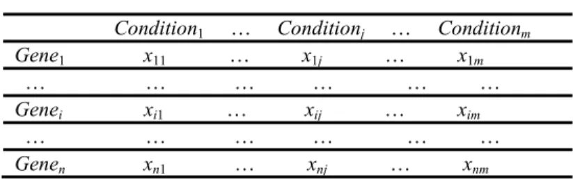
Analysis of gene expression data obtained from microarray experiments can be made through biclustering. Indeed, gene expression data are usually represented by a data matrix M (see Table.1), where the ith row represents the ith gene, the jth column
represents the jth condition and the cell xij represents the
expression level of the ith gene under the jth condition. In general,
subsets of genes are coexpressed only under certain conditions but behave almost independently under others. Discovering such coexpressions can be helpful to discover genetic knowledge such as genes annotation or genes interaction. Hence, it is very interesting to make a simultaneous clustering of rows (genes) and of columns (conditions) of the data matrix to identify groups of rows (genes) coherent with groups of columns (conditions), i.e., to identify clusters of genes that are coexpressed under clusters of conditions, or clusters of conditions that make clusters of genes coexpress. This type of clustering is called biclustering [6]. A cluster made thanks to a biclustering is called bicluster. Hence, a bicluster of genes (resp. conditions) is defined with respect to only a subset of conditions (resp. genes). Thus, a bicluster is a subset of genes showing similar behavior under a subset of
conditions. Let us note that a gene/condition can belong to more than one bicluster or to no bicluster.
In other words, a bicluster can be defined as follows: Let
I={1, 2, …, n} be a set of indices of n genes, J={1, 2, …, m} be a
set of indices of m conditions and X(I,J) be a data matrix associated with I and J. A bicluster associated with the data matrix X(I,J) is a couple (I’,J’) such that I’⊆ I and J’⊆ J.
Actually, biclustering is a special case of clustering. Indeed, in biclustering, genes are clustered according to their expression levels under a number of conditions, not necessarily all the conditions. While in clustering, genes are clustered according to their expression levels under all the conditions. Similarly, in biclustering, conditions are clustered according to the expression levels of a number of genes, not necessarily all the genes.
The biclustering problem can be formulated as follows: Given a data matrix X, construct a bicluster
B
opt associated withX such that:
f(Bopt) = maxB∈BC(X) f(B) (1)
where f is an objective function measuring the quality, i.e., coherence degree, of a group of biclusters and BC(X) is the set of all the possible groups of biclusters associated with X.
TABLE 1 Gene Expression Data Matrix.
Condition1 … Conditionj … Conditionm
Gene1 x11 … x1j … x1m
… … … … … …
Genei xi1 … xij … xim
… … … … … …
Genen xn1 … xnj … xnm
Clearly, biclustering is a highly combinatorial problem with a search space size O(2|I|+|J|). In its general case, biclustering is
NP-hard [6].
2
2 adopting a BMM and suggest a new fuzzy biclustering one. Our
approach enables to choose a good strategy of initialization of BEM and BCEM algorithms.
The rest of this paper is organized as follows: In sections II and III, we briefly review the different types of biclusters and groups of biclusters. In section IV, we present the Mixture Model (BMM). Section V is devoted to describe our new fuzzy biclustering approach. Finally, in section VI, we present our conclusion and perspectives
II.TYPES OF BICLUSTERS
A bicluster can be in one of the following cases:
1. Bicluster with constant values: It is a bicluster where all the values are equal to a constant c:
xij= c (2)
2. Bicluster with constant values on rows or columns: • Bicluster with constant values on rows: It is a bicluster where all the values can be obtained by using one of the following equations:
xij = c + ai (3)
xij = c ×ai (4)
Where c is a constant and ai is the adjustment for the
row i, 1 ≤ i ≤ n.
• Bicluster with constant values on columns: It is a bicluster where all the values can be obtained by using one of these equations:
xij =c + bj (5)
xij = c × bj (6)
Where c is a constant and bw is the adjustment for the
column j,1≤ j ≤ m.
3. Bicluster with coherent values: It is a bicluster that can be obtained by using one of the following equations:
xij = c + ai + bj (7)
xij = c × ai ×bj (8)
4. Bicluster with linear coherent values: It is a bicluster where all the values can be obtained by using the following equation:
xij = c × ai + bj (9)
5. Or, bicluster with coherent evolution: It is a bicluster where all the rows (resp. columns) induce a linear order across a subset of columns (resp. rows).
III.GROUPSOFBICLUSTERS
A group of biclusters can be in one of the following cases [13]:
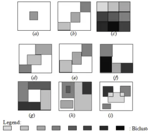
1. Single bicluster ((Figure 1 (a)),
2. Exclusive row and column group of biclusters (Figure 1 (b)),
3. Non-overlapping group of biclusters with checkerboard structure (Figure 1 (c)),
4. Exclusive rows group of biclusters (Figure 1 (d)), 5. Exclusive columns group of biclusters (Figure 1 (e)), 6. Non-overlapping group of biclusters with tree structure (Figure 1 (f)),
7. Non-overlapping non-exclusive group of biclusters (Figure 1 (g)),
8. Overlapping group of biclusters with hierarchical structure (Figure 1 (h)),
9. Or, arbitrarily positioned overlapping group of biclusters (Figure 1 (i)).
Figure 1 Possible structures of a group of biclusters in a data matrix.
A natural way to visualize a group of biclusters consists in assigning a different color to each bicluster and in reordering the rows and the columns of the data matrix so that we obtain a data matrix with colored blocks, where each block represents a bicluster.
IV.BLOCK MIXTURE MODEL
An attractive way to make biclustering of genes and conditions is to adopt a Block Mixture Model (BMM) [8, 10]. This presents the advantage of selecting an adequate model for each bicluster, which leads to biologically pertinent biclustering of gene expressions data.
A. Definition of the model
Mixture Models (MM) [8,10] are widely adopted in a variety
of areas and particularly in unsupervised learning. With a clustering approach based on a MM, it is assumed that the data to be clustered are generated by a mixture of underlying probability distributions in which each component represents a different cluster. Given observations X = (x1,…, xn),
the probability density function (pdf) is defined as follows: ) ; ( ) ; ( K 1 k k k i k i p x x f θ =
∑
= ϕ α , (10) where ϕk(xi;αk) is the density of an observation xi from the kth
component (cluster) and the pk’s, 1 ≤ k ≤ K, are the corresponding
cluster parameters. These densities belong to the same parametric family (spherical, diagonal or general family). A parameter pk,
(cluster), where K, assumed to be known, is the number of the components (clusters) in the mixture. The parameter of this model is the couple θ = (p,α), where p = (p1,…,pK) represents the
mixing proportions and α = (α1, …, αK) represents the
parameters of each component (cluster). The mixture density of the observation x is expressed as follows:
) ; ( ) ; ( Kk1 k k i k i p x x f θ =
Π
∑
= ϕ α . (11)Let z=( zik) be the (n × K) binary classification matrix indicating
the labels of rows into K clusters (zik =1 if the row i belongs to
the kth cluster and 0 otherwise). Govaert and Nadif [9] have shown that equation (10) can be written in the following way:
( ; ) ∑ ( ; ) ( ; , ) (12) where Z is the set of all possible assignments z of I and,
p( ; ) ∏, and ( ; , ) ∏, ( ; ) .
In the context of the biclustering problem, equation (13) takes the following expression:
( ; ) ∑( , ) Z W ( ; ) ( ; ) ( ; , , ) (14) where w=(wjl) corresponds to the (m × L) binary classification
matrix indicating the labels of columns into L clusters (wjl =1 if
the column j belongs to the lth cluster and 0 otherwise) while W denotes the set of all possible assignments w of J. A MM associated with equation (14) is called Block Mixture Model (BMM) [8, 10].
B. Soft and hard approaches
Approaches based on a BMM operate thanks to a Block
Expectation Maximization (BEM) algorithm and/or a Block Classification Expectation Maximization (BCEM) one [2].
Let’s note that BCEM algorithm differs from BEM one by the fact that we have inserted a classification step between estimation and maximization ones.
1) Block EM algorithm
A Block EM algorithm (BEM) has the same convergence properties as Generalized EM one [11]. And, like an EM one, a BEM algorithm converges slowly in some situations. The second important drawback of this kind of algorithms is that their solutions can highly depend on their starting position and, consequently, produce sub-optimal maximum likelihood estimates. To cope with this high dependency, Govaert and Nadif [11] have proposed to use the em-EM strategy to initialize parameters estimations of a BEM algorithm.
This strategy consists in several short runs of BEM from random positions followed by a long run of BEM from the solution maximizing the likelihood. A BEM algorithm can be defined as follows:
Step 1: Set r: = 0, choose s from [2..n] and t from [2..m]; Choose z(0), w(0) and θ(0) as initial values of z, w and θ
Step 2: Compute z(r+1), w(r+1) and θ(r+1) thanks to the alternated
application of EM on intermediate data matrices; for details see for instance [11].
Step 3: Iterate Step 2 until convergence.
2) Block CEM algorithm
As we said earlier, a BCEM algorithm differs from a BEM one by the fact that we have inserted a classification step between estimation and maximization ones. That is why, we need to adopt classification log-likelihood function Lc(z,w,θ) instead of
log-likelihood one L(z,θ). A BCEM algorithm [11] differs from a BEM one by the fact that in Step 2 we call a CEM algorithm instead of an EM one.
C. Fuzzy approaches
Hard approaches adopting a BMM present the following drawbacks:
(i) All initializations strategies, including em-EM, of parameters estimation adopted by hard approaches are still inefficient and therefore do not contribute to generate pertinent groups of biclusters, i.e., groups of biclusters with optimal values of ML/CML function.
(ii) These approaches converge slowly and therefore are time consuming.
(iii) Concerning hard approaches that operate separately on the sets of genes I and the sets of conditions J (denoted by 2EM and 2CEM), the correlations that exist between subsets of genes and subsets of conditions are ignored.
That is why researchers opted for fuzzy approaches adopting a BMM to deal with the biclustering problem. In this context, Govaert and Nadif [12] proposed Block Fuzzy C-Methods (BFCM) based on Neal and Hinton interpretation of EM [4]. The obtained approach enables to maximize a fuzzy clustering
criterion. Miin-Shen Yang and Chih-Ying Lin [5], on their side,
proposed a Block Fuzzy K-Modes (BFKM) clustering approach based on Huang and Ng Fuzzy K-Modes (FKM) approach [5].
1) Neal and Hinton interpretation of EM
As pointed out by Hathaway [3], in a classical MM context, an EM algorithm can be viewed as an alternated maximization of the following fuzzy clustering criterion:
( , θ) ( , θ) ∑, log (15)
where s is a n × g data matrix, with n is the number of genes and g is the maximum number of gene clusters to generate. The ith row
of s represents the ith gene, the kth column represents the kth cluster
and the cell sik expresses the probability that the ith gene belongs
to the kth cluster. The function
( , ) log( ( , ))
,
is the fuzzy complete data log-likelihood. Indeed, maximizing Lc
with respect to s, and consequently FC with respect to s, yields the
expectation step and maximizing Lc with respect to θ, and
consequently FC with respect to θ, yields the maximization one.
To extend this interpretation to all models in which an EM algorithm may be employed, Neal and Hinton [4] proposed to use the following function:
4
4 ( , θ) ( ( , θ)) + ( ) (16)
where z represents the missing data, P is a distribution over the space of z and H is an entropy function. One can also relate FC to
the Kullback–Leibler divergence between P(z) and ( ) ( ; , ), as follows:
( , θ) (θ) ( , P ) (17) The alternated maximization of the FC function is then simple
to set up:
(i) Maximization of FC(P,θ) with respect to P for fixed θ :
Equation (17) leads to the minimization of ( , )) and then to
P=Pθ.
(ii) Maximization of FC(P,θ) with respect to θ for fixed P:
Equation (16) shows that θ maximizes the expectation
Ep(Lc(z,θ)).
These two steps are precisely those of an EM algorithm. Moreover, after the first step, we have FC(P,θ) = FC(Pθ,θ) =
LM(θ), which shows that each iteration increases the
log-likelihood LM(θ).
One can easily see that the Neal and Hinton interpretation extends Hathaway’s relation (14). Indeed, for a classical MM, the missing data z represents the assignments of the genes of the set
Z, and the assignments of each xi obtained in the expectation step
are independent. Then, the conditional distribution P(z) is given by the vector that is the concatenation of the rows of the n×g data matrix s. Moreover, thanks to the Neal and Hinton interpretation [4, 5] of equations (15) and (16), Ep(Lc(z,θ)) can be transformed to
Lc(s,θ), and H(P) can be transformed to ∑, log .
For latent block model, Govaert and Nadif [13] adopted Neal and Hinton fuzzy criterion (15) defined by:
( , θ) ( ( , θ)) + ( ) (18) where ( , ; ) , + , + , , , ( ; )
2) Block Fuzzy C-Methods
In [12] the authors proposed Block Fuzzy C-Method (BFCM) as a new biclustering method based on a BMM and fuzzy c-partitions [1]. The new optimized objective function is defined as follows:
(
, ,
)
(
, ,
)
( )
,
c cF c d
θ
=
L c d
θ
+
H c d
(19) where ( , , ) ∑, log( ) + ∑, log( )+ logφ , , , , and ( , ) log( ) + log , ,where cik and djl represent the fuzzy partitions of genes and
conditions, respectively.
To maximize Fc(c,d;θ), in [12] the authors shown that this aim
can be performed by maximizing alternatively two conditional fuzzy criteria Fc(c,θ|d) and Fc(d,θ|c). Their maximization can be
viewed as an EM algorithm with a ML function associated with a classical MM on intermediate matrices. Thus, we can summarize BFCM algorithm as follows:
Step 1: Choose c(0), d(0) and θ(0) as initial values of c, d and θ Set r: = 0, choose s from [2..n] and t from [2..m];
Step 2: Compute c(r+1), d(r+1) and θ(r+1) thanks to the alternated
application of EM on intermediate data matrices. Step 3: Iterate Step 2 until convergence.
We present now the Block Fuzzy K-Modes (BFKM) clustering algorithm [5].
3) Block Fuzzy K-Modes algorithm
For clustering categorical data, i.e., types of data which may be divided into groups, Huang and Ng [5] proposed the Fuzzy
K-Modes (FKM) algorithm using simple matching dissimilarity
measures. Huang and Ng [5] added the concept of biclustering with FKM, and then proposed the Block FKM(BFKM) method.
Let Y = {y1,..,yn} be a set of data. Let each data be defined by a
set of attributes A1,…,Am such that yi= {yi1,..,yin}, i = 1,…,n. Each
attribute Aj , j = 1, … , J describes a domain of values denoted by
DOM(Aj)={aj(1) , …, aj(Lj)}where Lj denotes the cardinality of
DOM(Aj). Suppose that ( , . . , ) is the centroid of the
kth cluster where each component , … , for
k=1,…,K , j=1,…,L with 1 and 0 for l’≠l, 1≤j≤m,
1≤l’, l≤ Lj. Huang and Ng [8] used the following matching
dissimilarity measure:
∑
=∂
=
∂
J j ij kj k iy
y
d
1)
,
(
)
,
(
δ
(20) where ⎩ ⎨ ⎧ ∂ ≠ ∂ = = ∂ kj ij kj ij kj ij if y y if y , 1 , 0 ) , ( δThe fuzzy k-modes clustering algorithms is to minimize the following objective function:
∑∑
= =∂
=
∂
n i K k k i m ik md
y
H
1 1)
,
(
)
,
(
μ
μ
subject to ∑ 1For i = 1, …,n. The update equations for fuzzy k-modes are as follows: b>1, [0,1] and (∑ ( ( ( , ), )) ) . We note is the cluster center, it is defined by:
1, if ∑ ∑
0, otherwise Where f’ and l’ are the numbers of the attribute
A
j(21) The BFKM clustering algorithm aims at minimize the following objective function:
( , , , , , ) ( ) ( , )
,
+ ( ) ( , )
,
(22) Subject to ∑ 1 , for k=1,…, K and ∑ 1, for
j=1,…, L. and are respectively the clusters centers, X is a data matrix with n genes and m conditions, and Y is the transpose of X. The update equations for BFKM are as follows:
m1 > 1, m2 > 1, [0,1] , and [0,1]
(∑ ( ( ( , ), )) ) and (∑ ( (( , ), )) ) (23) We note and are the clusters centers, there are defined by: 1, if ∑ ∑ 0, otherwise (24) 1, if ∑ ∑ 0, otherwise (25)
Where f’ and h’ are the numbers of the attribute
A
j Thus, we can summarize BFKM algorithm as follows:Step 1: Set r: = 0, choose k from [2..K], l from [2..L] and ε from [0..0.5];
Choose µ(0) and σ(0) as initial values of µ and σ
Step 2: Compute µ(r+1), σ(r+1), (r+1), (r+1) from µ(r), σ(r), (r) and (r)
thanks to equations (23), (24) and (25). Step 3: If |µ(r+1)-µ(r)| + |σ (r+1)-σ (r)| < ε then stop
else set r := r + 1, go to Step 2.
V.ANEW FUZZY ALGORITHMADOPTING BMM
Both BFCM [12] and BFKM [5] algorithms present the following drawbacks:
(i) They do not really apply the principal of fuzzy logic. Indeed, they do not adopt Fuzzy Membership Functions (FMF).
(ii) To act against this high dependency on its initial position, in [12] the authors propose to use the "em-EM" strategy.
Unlike BFCM and BFKM algorithms, our biclustering algorithm:
(i) Really adopts FMF
(ii) Adopts fuzzy logic techniques in the strategy of initialization of parameters estimation. Indeed, fuzzy logic enables flexible initialization of parameters estimation.
Besides, we propose Fuzzy Logic Block Lazy EM algorithm (FLBLEM) to be adopted by our biclustering approach instead of BEM one. FLBLEM is based on a Lazy EM (LEM) [13] which is faster than EM. We can summarize our biclustering approach as follows:
During the first step, we fix a maximum number of biclusters, via the FMF, to initialize the parameters of our BMM.
During the second step, we cluster genes and/or conditions simultaneously, or consecutively, by applying a Block Lazy EM (BLEM) algorithm, if we are in an estimation phase.
During the last step, we tune the obtained group of biclusters either by merging biclusters or by creating others. If the algorithm does not converge, we repeat the second step.
V.CONCLUSION AND PERSPECTIVES
In this paper, we have reviewed existing biclustering approaches adopting a Block Mixture Model (BMM) and suggested a new fuzzy biclustering one.
Our approach enables to choose a good strategy of initialization of Block Expectation Maximization (BEM) and Block
Classification Expectation Maximization (BCEM) algorithms.
This an ongoing work, as perspectives, we have to: (i) Handle missing values in microarray data,
(ii) Speed-up our approach by defining a good strategy of choice of the initial number of biclusters.
(iii) Make an experimental study of our approach and compare the obtained results with those obtained by Block Fuzzy
C-Methods (BFCM) [12] and Block Fuzzy K-Modes (BFKM) [5]
ones.
REFERENCES
[1] E. Ruspini, “A new approach to clustering,” Information and Control, vol. 15, pp. 22-32, 1969.
[2] A.J. Scott and M.J. Symons, “Clustering methods based on likelihood ratio criteria,” Biometrics, vol. 27, pp. 387-397, 1971.
[3] R.J. Hathaway, “Another interpretation of the EM algorithm for mixture distributions,” Stat. and Probability Lett., vol. 4, pp. 53-56, 1986.
[4] R.M. Neal and G.E. Hinton, “A view of the EM algorithm that justifies incremental, sparse, and other variants”. In: Jordan, M.I. (Ed.), Learning in Graphical Models. Kluwer Academic Publishers, Dordrecht, pp. 355–358. 1998.
[5] Z. Huang, M. and K. Ng, “A fuzzy k-modes algorithm for clustering categorical data,” IEEE Transactions on Fuzzy Systems, vol. 7, pp. 446-452, 1999.
[6] Y. Cheng and G. M. Church, “Biclustering of expression data.”, in Proceedings of the Eighth International Conference on Intelligent Systems for Molecular Biology, pages 93{103. AAAI Press, 2000.
[7] B. Thiesson, C. Meek and D. Heckermand, “Accelerating EM for Large Databases”, Microsoft Research rapport noMSR-TR-99-31, 2001.
[8] A. Dharan and A. S. Nair. “Biclustering of gene expression data using reactive”.
[9] G. Govaert and M. Nadif, “Clustering with block mixture models,” Pattern Recognition, vol. 36, pp. 463-473, 2003.
[10] S.C. Madeira and A. L. Oliveira. “Biclustering algorithms for biological data analysis: A survey”. IEEE/ACM Transactions on Computational Biology and Bioinformatics (TCBB), 1(1):24{45, 2004.
[11] G. Govaert and M. Nadif, “An EM algorithm for the block mixture model”. IEEE Trans. Pattern Anal. Mach. Intell. 27, 643–647. 2005.
[12] G. Govaert and M. Nadif, “Fuzzy clustering to estimate the parameters of block mixture models,” Soft Computing, vol. 10, pp. 415-4220, 2006. [13] F.-X. Jollois and M. Nadif, “Speed-up for the expectation-maximization
algorithm for clustering categorical data”, Springer Science Business Media B.V. 2006.