Coupling between molecular rotations and OH***O motions in liquid water: Theory and experiment

(1)

HAL Id: hal-00836944

https://hal-polytechnique.archives-ouvertes.fr/hal-00836944

Submitted on 19 May 2014

HAL is a multi-disciplinary open access

archive for the deposit and dissemination of

sci-entific research documents, whether they are

pub-lished or not. The documents may come from

teaching and research institutions in France or

abroad, or from public or private research centers.

L’archive ouverte pluridisciplinaire HAL, est

destinée au dépôt et à la diffusion de documents

scientifiques de niveau recherche, publiés ou non,

émanant des établissements d’enseignement et de

recherche français ou étrangers, des laboratoires

publics ou privés.

Coupling between molecular rotations and OH*O**

motions in liquid water: Theory and experiment

Guilhem Gallot, S. Bratos, S. Pommeret, Noëlle Lascoux, J.-Cl. Leicknam, M.

Kozinski, W. Amir, Geoffrey Gale

To cite this version:

Guilhem Gallot, S. Bratos, S. Pommeret, Noëlle Lascoux, J.-Cl. Leicknam, et al.. Coupling

be-tween molecular rotations and OH***O motions in liquid water: Theory and experiment. Journal

of Chemical Physics, American Institute of Physics, 2002, 117 (24), pp.11301. �10.1063/1.1522378�.

�hal-00836944�

(2)

Coupling between molecular rotations and OH

_¯

O motions

in liquid water: Theory and experiment

G. Gallot

Laboratoire d’Optique et Biosciences, E´ cole Polytechnique, Route de Saclay, 91128 Palaiseau Cedex, France

S. Bratos

Laboratoire de Physique The´orique des Liquides, Universite´ Pierre et Marie Curie, 4 Place Jussieu, 75252 Paris Cedex 05, France

S. Pommeret

CEA/Saclay, DSM/DRECAM/SCM/URA 331 CNRS, 91191 Gif-sur-Yvette, France N. Lascoux

J-Cl. Leicknam and M. Kozin´ski

Laboratoire de Physique The´orique des Liquides, Universite´ Pierre et Marie Curie, 4 Place Jussieu, 75252 Paris Cedex 05, France

W. Amir and G. M. Gale

~Received 19 July 2002; accepted 25 September 2002!

A new theory is proposed to describe spectral effects of the coupling between molecular rotations and OH¯O motions in liquid water. The correlation function approach is employed together with a special type of development in which the coupling energy of these two motions is the expansion parameter. The isotropy of the liquid medium plays an essential role in this study. Based on this theory, a new infrared pump–probe experiment is described permitting a visualization of molecular rotations at subpicosecond time scales. Full curves relating the mean squared rotational angle and time, and not only the rotational relaxation time, are measured by this experiment. However, very short times where the incident pulses overlap must be avoided in this analysis. The lifetime of OH¯O bonds in water is rotation–limited. © 2002 American Institute of Physics.

@DOI: 10.1063/1.1522378# I. INTRODUCTION

The past decade has contributed much new information about short time hydrogen bond dynamics in liquid water. This is due to the development of new powerful lasers, gen-erating pico- and femto-second pulses in the mid-infrared spectral region. It now became possible to study this liquid, so essential for the life on our planet, on tiny time scales extending from a few hundreds of femto-seconds to a few tens of pico-seconds. Employing pump–probe techniques, the OH¯O motions in liquid water were studied in real time;1,2 the procedure was similar to that employed by Zewail et al. in their breakthrough work on the ICN dissociation.3,4 No oscillations of the hydrogen bond were detected. Moreover, the coupling between molecular rota-tions and OH¯O morota-tions in water was examined on the same time scales.5–7 The forces hindering them depend on the distance between the two oxygen atoms, which intro-duces a correlation between these degrees of freedom. From the other side, physico–chemical properties of various short lived structures present in liquid water were studied too: the hydrogen bond network generates irregularly fluctuating tetrahedral assemblies around each water molecule.8 –10 Fi-nally, recent photon echo experiments brought out

unexpect-edly fast dynamics of the OH¯O grouping, not yet seen before.11Femtochemistry of water thus remains a very active branch of science.

The purpose of the present paper is to pursue this effort by describing a new statistical theory of couplings between molecular rotations and the OH¯O motions. The correlation function approach is employed all along as well as a special type of expansion in which the energy of coupling between rotational and OH¯O motions is the expansion parameter. The isotropy of the liquid system plays a crucial role. Based on theoretical results, a new pump–probe experiment is pro-posed permitting to visualize HDO rotations in HDO/D2O

solutions in real time. Full curves relating mean squared ro-tational angles and times, and not only the roro-tational relax-ation time, are measured. However, the overlap of incident pulses at short times severely complicates the analysis. The lifetime of the OH¯O bonds in water is shown to be rotation limited.

II. GENERALITIES

Femtosecond dynamics of OH¯O bonds in water are most often studied by using ultrafast pump–probe tech-niques.1,2The procedure is based on a well-known

relation-11301

(3)

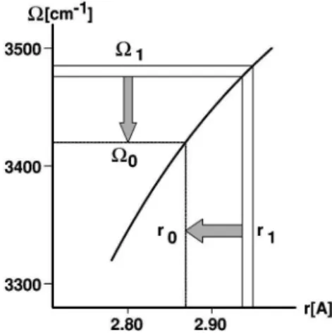
ship linking the hydrogen stretching frequency V of an OH¯O bond and its length r. The stronger the hydrogen bond, the softer the OH link and the lower is its frequency V. Following the initial proposal of Rundle and Parasol, a number of empirical relationships were published; the one adopted here is the recent relationship due to Mikenda12 il-lustrated in Fig. 1. The experiment then goes as follows. An ultrafast pump pulse of frequency V1, belonging to the

con-ventional OH stretching band of HDO, is used to excite OH vibrations; this excitation results in selecting OH¯O bonds of a given length r1. However, the system does not conserve

this nonequilibrium geometry, but returns progressively to the equilibrium; the OH¯O bond length then passes from its initial value r₁ to the equilibrium value r₀. Simultaneously, the OH band shifts from the pump frequency V₁ to its equi-librium frequency V₀. Thus, probing the position of the OH band as a function of the pump–probe delaytand using the Mikenda relation, the value of the OH¯O bond length can be deduced in each moment. It is thus possible to follow its temporal variations directly.

The above experiment was also adapted to the study of HDO rotations in liquid HDO/D2O solutions.5–7The method

consists in selecting hydrogen bonds of a specified length r1

by pumping the system with an appropriate frequency V1.

Molecular rotations of the subset of hydrogen bonds created in this way are analyzed next by measuring the rotational anisotropy R5(Si2S_')/(Si12S_') of the system for

differ-ent probe frequencies V2and for different time delayst; the

signals Si and S_'correspond to the parallel and

perpendicu-lar electric field configurations, respectively. This quantity is an important indicator of molecular rotations in liquid systems.13–15In fact, if ~i! the couplings between molecular rotations and other degrees of freedom are absent, and ~ii! the time delaytbetween the pump and probe pulses are long enough to avoid their overlap, then in very general conditions16,17

R~t!5~2/5!

^

P2~ cos~u~t!!!

&

5~ 2/5!exp~ 23/2

^

u2~t!

&

!, ~1!

where P2 is the second-order Legendre polynomial andu~t!

the angle between the transition moment vectors in times 0 andt. Measuring R(t) as a function of timetthus provides the square averaged rotation angle

^

u(t)2

&

; this experiment

has the intrinsic power of visualizing molecular rotations. The above relation simplifies for timestlong as compared to the correlation time of the molecular angular velocity v

5du/dt. Molecular rotations then transform into rotational diffusion, and Eq. ~1! takes the well known form R(t)

5(2/5)exp(2t/tO) where tO is the rotational relaxation

time. Measuring R(t) as a function oft in these conditions then providestO, but not the full curve

^

u(t)2

&

. Finally, it

should be stressed that this theory predicts R(t) to be inde-pendent of V1 and V2.

However, all these conclusions only apply if the condi-tions ~i!, ~ii! underlying the derivation of Eq. ~1! hold true. Are they satisfied in the case of water? The condition ~ii! certainly fails at smallt’s where the pump and probe pulses overlap, whatever the material under consideration. Unfortu-nately, the condition ~i! is not satisfied neither for water, although the coupling between molecular rotations and re-maining degrees of freedom may be absent in other liquids. In fact, R(t) was measured as a function of V1 and V2; it

was found to be distinctly V1, V2 dependent, which proves

the presence of couplings. How to proceed in these condi-tions? Can Eq. ~1! still be applied in spite of this difficulty? A possible, although approximate, way out is to maintain the expression R(t)5(2/5)exp(2t/tO) and to consider tO, or

equivalently the rotational diffusion constant DR, to depend on the OH¯O distance; R(t) then becomes in fact fre-quency dependent. However, introducing a model of this type, does not exempt one of the necessity to construct a fully statistical theory of couplings between molecular rota-tions and OH¯O morota-tions. The purpose of this paper is to present a theory of this kind.

III. THEORY A. Basic formulas

The system under consideration is a diluted isotopic so-lution HDO/D2O in thermal equilibrium. It contains N solute

molecules in a volume V. A pump pulse of frequency V1

brings the system in an excited state; and a probe pulse of frequency V2explores its return in its ground state at timet.

The pump and probe electric fields are E15(E1x,E1y,E1z)

and E₂_5(E_2x,E_2y,E_2z), and the total electric field is

E5(E1x1E2x,E1y1E2y,E1z1E2z). These two fields are

not parallel to each other in general.

The quantity measured experimentally is the pump– probe signal S(V₁,V₂,t). It is defined as the total probe absorption W(V1,V2,t) in presence of the pump minus the

probe absorption W(V2) in absence of the pump. Then, if

M( Mx, My, Mz) denotes the electric dipole moment of the system, the following formula applies:18,19

S~ V1,V2,t!5~2/\3!Im

E

2` `

E

0 `

E

0 `

E

0 ` dt dt1 dt2 dt3 3

^

E˙2i~ r,t !Ej~ r,t2t3! 3Ek~ r,t2t32t2!El~ r,t2t32t22t1!

&

E 3

^

Ml~ 0 !@ Mk~t1!,@ Mj~t11t2!, 3Mi~t11t21t3!##

&

S. ~2!

FIG. 1. Relation between the OH¯O hydrogen bond length r and the OH link frequency V. r0and V0designate the equilibrium values of r and V.

11302 J. Chem. Phys., Vol. 117, No. 24, 22 December 2002 Gallotet al.

(4)

This expression involves two kinds of 4-time correlation functions: the correlation functions of the total and the probe electric fields E~r,t! and E2(r,t) and those of the electric

dipole moment M(t) of the system. The indices i, j , k, l denote the Cartesian components of these vectors; the Ein-stein convention is employed all along indicating a summa-tion over doubled indices. The average

^ &

S is over states of the nonperturbed liquid system, and the average

^ &

E is over all possible realizations of the incident electric fields. The symbol @,# denotes a commutator and the dot a time deriva-tive. Choosing the electric fields E₁, E₂ of appropriate form, all possible cases of polarization may be treated. It should be noted that Eq. ~2! represents an exact third-order perturbation theory result.

B. Model

The above equation will now be employed to study ro-tational anisotropy of an isotopic water solution. The pump electric field E1(r,t)5(0,0,Epump(r,t)) is supposed to be

po-larized along the laboratory fixed z axis, and the probe elec-tric field to be either E2(r,t)5(0,0,Eprobe(r,t)) in the

paral-lel electric field configuration or E2(r,t)5(0,Eprobe(r,t),0)

in the perpendicular electric field configuration. The total electric field is then E(r,t)5(0,0,Epump(r,t)1Eprobe(r,t))

in the first case, and E(r,t)5(0,Eprobe(r,t),Epump(r,t)) in

the second. In all circumstances one has E_probe_!E_pump. Unfortunately, Eq. ~2! cannot be applied to the present case without approximations, and a model must be used; it involves the following assumptions: ~i! The OH vibrator of HDO/D2O is assimilated to a two-level quantum system,

per-turbed by random solvent–solute interactions. All remaining degrees of freedom of the system constitute a classical ther-mic bath. ~ii! Time evolution of the dipole moment M is governed by the modified Heisenberg equation

d dtM5

i

\@H,M#2GM, ~3!

where H is an adiabatic Hamiltonian and G the Pauli relax-ation operator. The ith component M_i of M is written M_i 5M ui, where M is the length of M and u its unit vector. The variable M is quantum-mechanical whereas u is classi-cal. ~iii! The pump and probe electric fields have slowly varying Gaussian amplitudes Epump(t), Eprobe(t) and random

phasesfpump(t), fprobe(t), independent of each other

Epump~ r,t !52 Re@Epump~ t

8

!

3exp~ ikpumpr2iVpumpt

8

!exp~ ifpump~ t

8

!!#,

~4! Eprobe~ r,t !52 Re@Eprobe~ t !

3exp~ ikprober2iVprobet !exp~ ifprobe~ t !!#,

where t

₈

_5t1t. Models of this type are of current use in laser physics. However, it only applies if the v50↔v51, but not the v51→v52, transition is involved in the experi-ment; a three-level model would be required otherwise. In practice, this means the excitation be must be confined to the 3500 cm21_{spectral region.}

The above model still needs to be completed by

present-ing time scales of the problem. The hydrogen bond dynamics in liquid water are controlled by three relaxation times. The first of them is the life timetp of the OH vibrator in its first excited state. It is surprisingly short: according to the most recent determinations it is of the order of 1.0 ps.1,2,9,10,20 Another characteristic time is the solvent relaxation timetV:

intermolecular forces are feebly modified by vibrational ex-citation, which leads to a rupture of thermic equilibrium. Experiment and molecular dynamics simulations proposed values of the order of 0.7 ps for it.1,2,21–25Finally, the rota-tional relaxation time tO measures the progressive loss of

orientational coherence; it corresponds to the correlation time of the second spherical harmonics. Involved in many experimental situations, it has been measured or calculated by a number of authors.26 –31The values of the order of 2.5 ps may be considered as representative. A last time playing a role in the present context, although only indirectly, is the dephasing time td: this is the time in which the phase co-herence of the nOH vibrations is lost due to the frequency

dispersion, and is of the order of 15 fs. It results from the above data that very short laser pulses, not longer than a few hundreds of femtoseconds, are required in this study. For convenience, the paper is written as to permit to skip, at first reading, the technical details which follow and pass to Sec. IV directly.

C. Dipole moment correlation functions 1. Liouville pathways of the system

It is convenient to start this calculation by studying di-pole moment correlation functions. As the coupling between rotations and OH¯O motions has to be fully accounted for, a considerable effort is required to do it. The calculation involves the following steps. ~i! The dipole moment of the system is written M5M u, where M is quantum-mechanical and u classical. Then:

^

Ml~ o !@ Mk~t1!,@ Mj~t11t2!,Mi~t11t21t3!##

&

S

5

^

ul~ 0 !uk~t1!uj~t11t2!ui~t11t21t3!

3M ~ 0 !@ M ~t1!,@ M ~t11t2!,M ~t11t21t3!##

&

S. ~5!

The quantities ui, uj, uk, ul are Cartesian components of the unit vector u; as they are classical, they may be shifted at will. The operation

^ &

S involves the average over the quan-tum states of the OH vibrator as well as that over the bath degrees of freedom; one has

^ &

S5

^

Trr

&

, where r is the vibrational density matrix and ^ & designates the averaging over the bath. ~ii! The incident electric fields are polarized either along the z or along the y axis. In these conditions, correlation functions in which the indices i, j, k, l are all equal to z, as well as those in which two indices are equal to y and two to z only survive. This is a consequence of the isotropy of a liquid system. ~iii! The above expression for correlation functions can be given a more explicit form by developing it over the quantum states of the OH vibrator. The matrix elements M00 and M11 do not contribute to the

OH band intensity and can safely be neglected. The matrix elements M01(t) and M10(t)5M01(t)* may be determined

by solving Eq. ~3!, which gives M (t)015M01

3exp@2i*0

t

dtv(t)2Gt# where \v_5H112H00. Then, if only

the ground vibrational state is thermally occupied, one finds

(5)

^

M_l~ 0 !@ Mk~t1!,@ Mj~t11t2!,Mi~t11t21t3!##

&

S 52~ M01M10!2exp~ 23Gt122Gt22Gt3! 3

H

K

ul~ 0 !uk~t1!uj~t11t2!ui~t11t21t3!exp

F

i

E

0 t1 dt v~ t !

G

_2i

E

0 t11t2 dt v~ t !

G

_1i

E

0 t11t21t3 dt v~ t)

&

1

K

F

i

E

0 t11t21t3 dt v~ t !2i

E

0 t11t2 dt v~ t !1i

E

0 t1 dt v~ t !

G

L

2

K

F

i

E

0 t11t2 dt v~ t !2

E

0 t11t21t3 dt v~ t !1

E

0 t1 dt v~ t !

G

L

2

K

F

i

E

0 t1 dt v~ t !2i

E

0 t11t21t3 dt v~ t !1i

E

0 t11t2 dt v~ t !

G

L

J

. ~6!

The four terms entering in this expression correspond to four different pathways in the Liouville space of operators.32

2. Series expansion for rotation–vibration correlations

Where are the effects of the rotation–vibration correla-tion hidden? In their absence, the terms of Eq. ~6! would all factorize into a rotational and a vibrational correlation func-tion, respectively; this is usually assumed to be legitimate. On the contrary, if the correlation is present, this step is strictly forbidden. A method must then be invented to treat the problem in its increased complexity. The one employed here consists of introducing a particular sort of series expan-sion, the principle of which is as follows.33 Let X and Y be two correlated stochastic variables and l a real number. Moreover, let the average over the stochastic process (X,Y ) be designated by ^ &. Then, using the cumulant expansion theorem and expressing the cumulant average by the symbol

^ &

c, one can write

I~ l !5

^

exp~ iX1lY !

&

⇒

S

dI dl

D

l50

5

^

Y exp~ iX !

&

,

I~ l !5exp

F

^

iX1lY

&

c1

1 2!

^

~ iX1lY ! 2

&

c 1_3!1

^

~ iX1lY !3

&

c1¯

G

⇒

^

Y exp~ iX !

&

[

S

dI dl

D

l50 5

F

^

Y

&

c1 i

^

XY

&

c2 1 2

^

X 2_Y

&

c1¯

G

3

^

exp~ iX !

&

. ~7!

This is the series expansion which was desired. Its leading term

^

Y

& ^

exp(iX)

&

expresses the average

^

Y exp(iX)

&

in ab-sence of correlation; and its higher order terms i

^

XY

&

c

^

exp(iX)

&

,21/2

^

X2Y

&

c

^

exp(iX)

&

, etc., describe the correlation effects. The stronger the correlation, the slower is the convergence. On the contrary, only the zero and first

order terms need to be considered if it is weak. This last condition will be taken as granted in what follows.

The above technique will now be applied in the present study. In fact, the terms in curly brackets of Eq. ~6! can all be given the form

^

Y exp(iX)

&

by simply choosing the variables X,Y properly. It suffices to take X

5*0 t1_dt_v_(t)2* 0 t11t2_dt _v_(t)1* 0 t11t21t3_dt _v_(t) _and _Y

5ul(0)uk(t1)uj(t11t2)ui(t11t21t3) in its first term,

and to proceed similarly in the three others. The problem then reduces to that of determining the averages

^

Y

&

c,

^

XY

&

c,

^

exp(iX)

&

for each possible choice of X,Y , i.e., for each Liouville pathway of the system. Detailed calculations are given below.

3. Details of calculations

One starts by calculating the quantities

^

exp(iX)

&

. They represent vibrational 4-time correlations functions in absence of rotation–vibration coupling. Occurring frequently in vari-ous domains of nonlinear spectroscopy, these functions are well known; see, e.g., Refs. 32 and 34. The cumulant expan-sion theorem leads to the following result:

^

exp~ iX !

&

5eiv0(t16t3)_exp

F

₂

1 2

E

0 t1

E

0 t1 dt dt

₈

b~ t,t

₈

! 21₂

E

0 t3

E

0 t3 dt dt

₈

b~ t,t

8

! 6

E

0 t1

E

0 t3 dt dt

₈

b~ t1t11t2,t

8

!

G

, ~8!

where v05

^

v

&

is the mean frequency of the transition v

51→v50 in solution, and b(t,t

₈

)5

^

v(t)v(t

₈

)

&

c is the

frequency shift correlation function; in what follows, it will be given a simple exponential form b(t)5

^

v2

&

c

3exp(2t/tV). The signs 6 depend on the Liouville pathway

which was chosen. Vibrational correlation functions vanish for t1,t3 large as compared to td andtV.. These variables

are thus limited which is important for subsequent develop-ments of the theory.

The quantities

^

Y

&

care studied next. They correspond to various rotational 4-time correlation functions in absence of

(6)

rotation–vibration coupling. For example,

^

Y

&

c is equal to

^

uz(0)uz(t1)uz(t11t2)uz(t11t21t3)

&

in the parallel

electric field configuration, whatever the Liouville pathway; this simplicity is lost in the perpendicular electric field con-figuration. The dependence of these functions ont1, t3 can

safely be suppressed: these variables are limited by the times

td,tV, which in their turn are small compared to the

rota-tional relaxation time tO. The resulting 2-time correlation

functions may be calculated by assuming that dynamic vari-ables uluk2

^

uluk

&

, etc., obey the simple Langevin equation of motion. Proceeding in this way one finds

^

uz~ 0 !uz~ 0 !uz~t2!uz~t2!

&

519~ 11 4 5e2zt2! ~i!,

^

uz~ 0 !uz~ 0 !uy~t2!uy~t2!

&

5 1 9~ 12 2 5e2zt2! ~'!, ~9!

^

uz~ 0 !uy~ 0 !uz~t2!uy~t!

&

5 1 15e2zt2 ~'!,

wherez51/tO. The first of these three rotational correlation

functions occurs in problems in which the pump and probe electric fields are parallel to each other, and the latter two are present in those in which the two fields are perpendicular.

Finally, the quantities

^

XY

&

c still remain to be treated. As they express rotational–vibrational coupling effects, they are central objects of the present theory. Their form varies when going from one Liouville pathway to another, but their general aspect is always the same,

^

XY

&

c56i

E

0 t1 dt

_8^

u_l~ 0 !uk~t1!uj~t11t2! 3ui~t11t21t3!Dv~ t

8

!

&

1i

E

0 t3 dt

_8^

ul~ 0 !uk~t1!uj~t11t2! 3ui~t11t21t3!Dv~ t

8

1t11t2!

&

, ~10!

where Dv(t)5v(t)2

^

v

&

. Detailed calculations involve the following steps. ~i! The variablest1,t3, and t

8

entering into

the 5-time correlation functions of Eq. ~10! are limited by the times td,tV. From the other side, the correlation times

as-sociated with them are expected to be of the order of, or only slightly smaller than tO. Then, as td,tV are small as

com-pared totO, the dependence ont1, t3, and t

8

may be

sup-pressed in all integrands, and the 5-time correlation functions become simple 2-time correlation functions. This time scale argument reduces massively the complexity of the problem, and makes calculations practicable. ~ii! The variables uluk 2

^

ulukDv

&

, etc., are supposed to obey the simple Langevin equation of motion, and to decay with the same decay con-stant z

8

. The quantities

^

u_z2Dv

&

,

^

u4_zDv

&

, and

^

u_z2u_y2Dv

&

which appear in the calculation can be determined by con-sidering the isotropy of the liquid medium. One finds, for example,

^

Dv

&

5

^

Dv(u_x2_1u2_y_1u_z2)

&

50⇒

^

Dvu_z2

&

50, etc. Setting a5

^

uz

4_D_v

&

there results

^

XY

&

c52ia~ 6t11t3!exp~ 22z

8

t2! ~i!,

~11!

^

XY

&

c5

1

2ia~ 6t11t3!exp~ 22z

8

t2! ~'!.

The upper of the above two expressions for

^

XY

&

cis valid if

the electric fields E₁,E₂ are parallel to each other, and the lower if they are perpendicular. From the other side, the signs 6 refer to different Liouville pathways of the system, i.e., to different terms in curly brackets of Eq. ~6!. Rotation– vibration coupling effects thus depend on the 2-time correla-tion funccorrela-tion

^

u_z2(0)u_z2(t2)Dv(t2)

&

5a exp(22z2

8

t2) and

vanish at times t2 such that t2@1/z

8

. The quantity a can

thus be interpreted as a rotation–vibration coupling constant. Astonishingly enough, in spite of its complexity the present analysis leads to comparatively simple, although nontrivial, results. Treating this complexity–simplicity is entirely sub-mitted to the isotropy of liquid medium.

The final expressions for dipole moment correlation functions may be obtained by collecting the above results for

^

exp(iX)

&

,

^

Y

&

c, and

^

XY

&

c. The sums (

^

Y

&

c1

^

XY

&

c) exp(iX) have to be evaluated for all possible Liouville path-ways, i.e., for each of the four terms of Eq. ~6!. As stated earlier, the dipole moment correlation functions required for determination of rotational anisotropy in present conditions are those which correspond to the indices zzzz, zzy y , z y z y , and z y y z; other combinations of indices i, j,k,l are irrel-evant for the present problem. This ends the study of dipole moment correlation functions in the presence of rotational– vibrational couplings.

D. Electric field correlation functions

The calculation of these functions is based on the fact that the wavelength l of the optical radiation is much longer than molecular dimensions, but much smaller than experi-mental cell dimensions. However, molecular motions are probed over distances l!l. A system experiencing a spa-tially varying electric field is then dynamically equivalent to an ensemble of subsystems submitted to a spatially constant electric field, but different when going from one subsystem to another. The vector r in E1(r,t), E2(r,t) no longer

de-notes a space point, but selects a given subsystem. It is thus legitimate to work with a spatially constant electric fields and to average the results over r at the end of the calculation. If the incident electric fields are coherent, the electric field correlation function takes its simplest possible form. Re-calling that in the parallel electric field configuration the pump and probe electric fields are E1(r,t)

5(0,0,Epump(r,t)) and E2(r,t)5(0,0,Eprobe(r,t)), whereas

in the perpendicular electric field configuration they are

E₁(r,t)5(0,0,Epump(r,t)) and E25(0,Eprobe(r,t),0), one

finds

^

E˙2i~ r,t !Ej~ r,t2t3!Ek~ r,t2t32t2!El~ r,t2t32t22t1!

&

5

(

s

(

t

(

u

CstuEprobe* ~ t !Eprobe~ ts!Epump* ~t1tt!

3Epump~t1tu!exp~ iVprobe~ t2ts!1iVpump~ tt2tu!!,

~12! where t15t3, t25t2t32t2, t35t2t32t22t3 and Cstu are constant coefficients; the indices sÞtÞu run from 1 to 3. These coefficients Cstu depend on the choice of i, j, k, l. They are thus different according to whether the function

(7)

under consideration is

^

EzEzEzEz

&

,

^

EyEyEzEz

&

,

^

EyEzEyEz

&

, and

^

EyEzEzEy

&

. As stated earlier, Eq. ~12! only applies if the laser fields are coherent. If they are not, the quantity between the square brackets must still be aver-aged over the random processes which are at the origin of the incoherence. The results depend on the physical nature of this latter process. This ends the study of 4-time electric field correlation functions; for a more detailed discussion, see the review in Ref. 18.

E. Numerical integrations

Before starting numerical work, various numerical data must still be fixed. Different relaxation times entering into the definition of dipole moment correlation functions were taken, whenever possible, from the published computer simulation work. This is true for the solvent relaxation time

tVand the rotational relaxation timetO. The value of 0.7 ps

was adopted for the former as suggested by Diraison et al.;22 and the value of 2.5 ps was ascribed to the latter, following Impey et al. as well as many others.27 Unfortunately, this purely theoretical attitude could not be maintained up to the end. Computer simulated population relaxation timestp are not accurate enough and the constantsa,z

8

were never cal-culated. tp was thus transferred from our previous experiments1,2 where it was given the value of 1.3 ps, 1/z

8

was assimilated to tO, and a constantaof 20.7 cm21

per-mitted to fit the experimental data. The duration of the inci-dent pulses was supposed to be 150 fs for both pump and probe; and the phases fpump(t), fprobe(t) were assumed to

be slowly modulated.

It remains to sketch procedures employed to perform multidimensional integrations over the variables t,t1,t2,t3

involved in Eq. ~2! for S(V1,V2,t). The integration over

the variable t appearing only in the field’s terms was realized analytically using a symbolic computation software ~Maple!. The integration over t1, t2, t3 was performed numerically

by employing the Romberg integration method, after two changes of variables on eachti. Proceeding in this way, an extremely robust and fast integration C11 program was provided from a large number of analytical expressions given by Maple. The time needed to compute a time step on a personal computer was of the order of a second. This method of integration can easily be extended to any nonlinear experi-ment such as photon echo or transient grating.

IV. THEORETICAL RESULTS

The principal results of the present theory will now be described. The main questions requiring a theoretical inter-pretation are as follows: Which are spectral effects of corre-lations between molecular rotations and the OH¯O motions in HDO/D2O solutions? What happens at the very shortest

times? Does rotational anisotropy R(t) permit a real time visualization of molecular rotations in presence of correla-tions? A first flavor of what the final answer could be comes from a theory generated result stating that, even if HDO rotations and OH¯O motions are correlated, the quantity Si12S_' remains independent of rotational dynamics,

whereas Si– S_'does depend on it. This can easily be proved

by adding in Eq. ~11! for

^

XY

&

c the first expression and twice the second; this sum vanishes. One concludes that at least some basic properties of R(t) survive in presence of correlations. This result is due to the isotropy of the liquid medium, and is by no means model dependent.

A more complete answer to the above questions is con-tained in Fig. 2; the insert illustrates the simple theory in absence of correlations. The following comments refer to two-color experiments realized at a fixed Vpumpand variable

Vprobe’s. ~i! Three time domains have to be distinguished.

The first of them corresponds to times t,200 fs: the pump and probe pulses overlap, or overlap partially, in this region. The second extends from 200 to 1500 fs, approximately: the pump-generated wave packets are available in a great num-ber, as are the compressed or elongated OH¯O bonds. Fi-nally, in the third time domaint_{.1500 fs, the wave packets}

are destroyed and the statistical equilibrium is reached again.

~ii! In the first domain, ln(R(t)) deviates from the limiting

value of ln~2/5!, increasing or decreasing at negativet’s as a function of Vprobe. This seemingly erratic behavior, not yet

reported in the literature, is due to the pump–probe coher-ence and is illustrated in Fig. 3. The dotted curves designate the anisotropy calculated by the complete theory, and the full curves that obtained by neglecting the coherent contribu-tions. The ‘‘anomalous’’ behavior of R(t) at shortt’s disap-pears in the latter case. ~iii! In the second time domain, ln(R(t)) measures the square averaged rotation angle

^

u2₍_t₎

_&

of the OH link. These rotations cannot be assimilated to a rotational diffusion: the dependence of

^

u2₍_t₎

_&

_on _t _{is not}

linear. Rotational anglesu~t! are smaller for the low than for the high V_probe’s; this behavior was expected:5–7 hydrogen bonds ‘‘seen’’ are shorter in the former case than in the latter ~Fig. 1!. ~iv! In the third time domain, a family of parallel straight lines with a slope corresponding to tO52.5 ps is

observed. Individual straight lines are shifted vertically with respect to each other, as a function of Vprobe; the straight

lines corresponding to small probe frequencies are placed higher than those associated with large ones. This observa-FIG. 2. Schematic presentation of R in presence of rotation–vibration cou-pling effects. The insert reproduces the results of the simple theory. Coher-ent effects dominate in the time domain 1, wave packet dynamics governs the time domain 2, whereas rotational diffusion is characteristic of the time

domain 3. In this figure Vprobe 1and Vprobe 2represent two values of the

probe frequency Vprobe.

(8)

tion indicates that in this time period water molecules ex-ecute a normal rotational diffusion with a normal relaxation timetO. However, the short time memory of the system is

not entirely lost: molecules having rotated faster in the sec-ond time period are deflected more than those which were slower, and the corresponding straight lines lie lower. An approximate analysis permits to guess the size of this effect: if the difference of the probe frequencies is equal to DV, the separation of the straight lines is equal to D(ln(R))

5~45/4!~a/b!~DV!. The experimentally obtained coupling

constanta is negative: the hydrogen bonds shorter than the average of 2.86 A thus contribute more to the coupling con-stant than the long hydrogen bonds.

In summary, three main effects are predicted by this theory. The first is that correlations between rotations and OH¯O motions transform an initially unique curve R 5R(t) into a family of curves R5R(t,Vpump,Vprobe). This

effect can be considered as a signature of correlated motions. The second effect is the interference of the pump and probe pulses at short times where they overlap. Rotational anisot-ropy R(t,Vpump,Vprobe) no longer remains a useful indicator

of rotational dynamics at these time scales. Finally, if this short time domain is eliminated, rotational anisotropy per-mits to visualize molecular rotations even if correlations are present. In fact, outside the overlap region, the quantity ln R(t,V_pump,V_probe)2ln(2/5) is still equal to 3/2 times

^

u2₍_t₎

&

at given V_pump,V_probe. Then using the relation of Fig. 1, the curves just described may be transformed into those relating

A

^

u2₍_t₎

_&

_and _t_{. A monocolor experiment is}

required to monitor molecular rotations in hydrogen bonds of a fixed length; a two-color experiment is needed to follow these motions in contracting or expanding hydrogen bonds. One concludes that, if the necessary precautions are taken, ultrafast laser spectroscopy permits to ‘‘film’’ molecular ro-tations in water.

V. VISUALIZING MOLECULAR ROTATIONS IN REAL TIME

In view of the very explicite nature of the above state-ments, it was decided to check them experimentally. A

pump–probe experiment was thus set up having the follow-ing characteristics: Its central element was a titanium– sapphire amplifier, delivering 130 fs pulses at 800 nm with a repetition rate of 1 kHz. It drived two lines of pulses, tuned independently in the midinfrared. The principle of the gen-eration was the parametric amplification of a quasicontinuum in the near infrared, followed by a frequency mixing in the midinfrared. The features of the sources were as follows. The more energetic line ~the pump! produced pulses having du-ration of 150 fs and a spectral width of 65 cm21. It delivered more than 10mJ between 2800 and 4800 cm21. The weaker line ~the probe! had similar characteristics but with a maxi-mum energy 10 times less. A motorized optical delay line precisely controlled the delay between the pump and the probe. In order to measure the anisotropy, the probe was turned at 45° from the pump by a midinfrared half-wave plate; the state of polarization was controlled by filtration after a Glan–Taylor prism, which compensated for a possible ellipticity of the outgoing beam. The sample was 100 mm thick and contained 1% HDO in D₂O at room temperature; it was circulated to avoid heating problems. It should be stressed that this experiment is intrinsically difficult. The an-isotropy R being defined as a ratio of two signals, the error bars become excessive whenever the latter are weak; this is always the case for negative pump–probe delay times as well as for times exceeding 2 ps. Nevertheless, the results are of a good quality in the interval between 0 and 2.5 ps; the accu-racy is smaller out of this interval.

The anisotropy curves obtained with excitation at 3510 cm21 _{are illustrated in Fig. 4. In spite of the complexity of}

the present problem, the agreement between theory and ex-periment is excellent. The theory can thus be accepted with much confidence. Finally, two ‘‘films’’ showing molecular rotations are given in Fig. 5. The mean squared rotational angle

A

^

u2₍_t₎

&

of the OH bond of HDO is illustrated as a function of timet. The OH¯O bond length is kept constant and equal to 2.99 A in curve ~a!, whereas it contracts from 2.99 A to 2.86 A in curve ~b!. One notices that rotational angles of the order of 35° are attained in times of the order of 700 fs. As a bending of this magnitude leads to a breaking of

FIG. 3. Rotational anisotropy R(t,V1,V2)calculated by the full theory

~dotted curves! and by a theory in which the coherent contributions are

suppressed ~full curves!. The pump frequency Vpumpis equal to 3510 cm21

and Vprobefrequencies are equal to ~a! 3510, ~b! 3450, and ~c! 3410 cm21,

respectively.

FIG. 4. ~Color! Rotational anisotropy R measured experimentally ~symbols O,h, n, L!, and calculated theoretically ~full curves!. The pump frequency Vpumpis equal to 3510 cm21, and the probe frequencies Vprobeare equal to

3510, 3480, 3450, and 3410 cm21_{, respectively.}

(9)

hydrogen bonds, one concludes that their lifetime in water is rotation limited. Unfortunately, our camera is blind at very short times where the pump and probe interact coherently: no ‘‘filming’’ is possible at those time scales. Note however that

A

^

u2₍₀₎

_&

_{is larger than zero for any finite pump and probe}

pulse duration. It is thus possible to ‘‘film’’ the HDO rota-tions in HDO/D2O solutions. Not only the OH¯O stretching

motions but also the HDO rotations can be monitored by ultra-fast laser spectroscopy. Here again, the original Zewail approach proves extremely useful in visualizing molecular motions.

VI. DISCUSSION

Only a limited number of papers have yet been pub-lished concerning the coupling between molecular rotations and OH¯O motions. In fact, the discovery of this subtle effect is recent5–7 and its analysis remains partial. The fol-lowing points merit attention. ~i! The theory was first elabo-rated in a semiempirical form. A model was proposed in which the reorientation time is supposed to depend on fre-quency and in which the spectral diffusion is incorporated. Formulated in this way, the model was able to confirm that water molecules rotate in fact slower in short hydrogen bonds than in long ones. The activation energy of molecular reorientations was also derived.6 However, the notion of an r-dependent rotational relaxation timetOremains to be

pre-cised. ~ii! The possibility of monitoring rotational anglesu~t! as a function ofthas been also envisaged in classical infra-red and Raman spectroscopy. However, their band shapes depend on rotational and on vibrational dynamics, simulta-neously. The two types of motion must thus be disentangled from each other, if rotations are to be studied. This is usually done by employing the so-called VV–VH separation technique.16Rotational self-correlation functions obtained in this way are

^

P1(cos(u(t)))

&

for infrared and

^

P2(cos(u(t)))

&

for Raman; the latter is exactly the same as in pump–probe experiments. Rotational angles u~t! can thus be, and have

occasionally been, determined by employing the two classi-cal techniques. Of course, the OH¯O bond length selection is impossible in this case. For further reading, see Ref. 35.

~iii! Molecular dynamics simulations of

^

P1(cos(u(t)))

&

and

^

P2(cos(u(t)))

&

showed that these functions exhibit a bump

at time scales of the order of 100 fs; it was attributed to librational dynamics of water molecules; see Refs. 27 and 31 and many others. Unfortunately, this interesting feature is undetectable by the present technique. The present discus-sion may be closed by emphasizing the importance in the present context of short time domains below 200 fs. Normal-izing the anisotropy to 2/5 at zero time propagates experi-mental errors to the rest of the spectrum and should be avoided.

ACKNOWLEDGMENTS

The authors gratefully acknowledge the support of the GDR 1017 of the CNRS during this work. The Laboratoire d’Optique et Biosciences is a Unite´ Mixte de Recherche No. 7645 of the CNRS and the Laboratoire de Physique The´or-ique des Liquides is a Unite´ Mixte de Recherche No. 7600 of the CNRS.

1_{G. Gale, G. Gallot, F. Hache, N. Lascoux, S. Bratos, and J-Cl. Leicknam,}

Phys. Rev. Lett. 82, 1068 ~1999!.

2_{S. Bratos, G. Gale, G. Gallot, F. Hache, N. Lascoux, and J-Cl. Leicknam,}

Phys. Rev. E 61, 5211 ~2000!.

3_{M. Dantus, M. Rosker, and A. H. Zewail, J. Chem. Phys. 87, 2395 ~1987!.} 4_{R. Bernstein and A. H. Zewail, J. Chem. Phys. 90, 829 ~1989!.} 5_{S. Woutersen, U. Emmerichs, and H. Bakker, Science 278, 658 ~1997!.} 6

H. K. Nienhuys, R. V. Santen, and H. Bakker, J. Chem. Phys. 112, 8487

~2000!.

7_{H. Bakker, S. Woutersen, and H. K. Nienhuys, Chem. Phys. 258, 233}

~2000!.

8_{H. Graener, G. Seifert, and A. Laubereau, Phys. Rev. Lett. 66, 2092}

~1991!.

9_{R. Laenen, C. Rauscher, and A. Laubereau, Phys. Rev. Lett. 80, 2622}

~1998!.

10_{R. Laenen, C. Rauscher, and A. Laubereau, J. Phys. Chem. B 102, 9304}

~1998!.

11

J. Stenger, D. Madsen, P. Hamm, E. T. J. Nibbering, and Th. Elsaesser, Phys. Rev. Lett. 87, 027401 ~2001!.

12_{W. Mikenda, J. Mol. Struct. 147, 1 ~1986!.} 13_{T. Tao, Biopolymers 8, 609 ~1969!.} 14

G. Fleming, J. Morris, and G. Robinson, Chem. Phys. 17, 91 ~1976!.

15_{A. Tokmakoff, J. Chem. Phys. 105, 1 ~1996!.}

16_{S. Bratos and E. Mare´chal, Phys. Rev. A 4, 1078 ~1971!.}

17_{J. S. Baskin, M. Chachisvilis, M. Gupta, and A. H. Zewail, J. Phys. Chem.}

102, 4158 ~1998!.

18

S. Bratos and J-Cl. Leicknam, J. Chim. Phys. Phys.-Chim. Biol. 93, 1737

~1996!.

19_{S. Bratos and J-Cl. Leicknam, J. Chem. Phys. 109, 9950 ~1998!.} 20_{H. K. Nienhuys, S. Woutersen, R. V. Santen, and H. Bakker, J. Chem.}

Phys. 111, 1494 ~1999!.

21_{S. Woutersen and H. J. Bakker, Phys. Rev. Lett. 83, 2077 ~1999!.} 22_{M. Diraison, Y. Guissani, J-Cl. Leicknam, and S. Bratos, Chem. Phys.}

Lett. 258, 348 ~1996!.

23_{A. Geiger, P. Mausbach, J. Schnitker, R. L. Blumberg, and H. Stanley, J.}

Phys. ~France! 45, C7 ~1984!.

24_{J. Marti, J. Padro, and E. Guardia, J. Chem. Phys. 105, 639 ~1996!.} 25_{A. Luzar and D. Chandler, Nature ~London! 379, 55 ~1996!.}

26_{M. Nakahara, in Physical Chemistry of Aqueous Solutions, edited by H.}

White, J. Sengers, D. Neumann, and J. Bellows ~Begell House, New York, 1995!, p. 449.

27_{R. Impey, P. Madden, and I. McDonald, Mol. Phys. 46, 513 ~1982!.}

FIG. 5. Real time ‘‘filming’’ of HDO rotations. The measured quantity is the

mean squared rotation angleA^u2₍_t₎_&_{of the OH bond of HDO at time}_t_,

starting from the initial OH bond direction; this angle is measured in de-grees. The OH¯O bond length is equal to 2.99 A in the curve ~a!, whereas it contracts from 2.99 A to 2.86 A in the curve ~b!. As expected, the OH rotations are slower in short OH¯O bonds.

(10)

28_{H. Berendsen, J. Grigera, and T. Straatsma, J. Phys. Chem. 91, 6269}

~1992!.

29_{K. Watanabe and M. Klein, Chem. Phys. 131, 157 ~1989!.} 30

D. V. Belle, M. G. Froeyen, G. Lippens, and S. Wodak, Mol. Phys. 77, 239

~1992!.

31_{I. Svishchev and P. Kusalik, J. Phys. Chem. 98, 728 ~1994!.}

32_{S. Mukamel, Principles of Nonlinear Optical Spectroscopy ~Oxford}

Uni-versity Press, New York, 1995!.

33_{G. Tarjus and S. Bratos, Phys. Rev. A 30, 1087 ~1984!.} 34

S. Bratos and J-Cl. Leicknam, J. Chem. Phys. 101, 4536 ~1994!.

35_{W. C. Rothschild, Dynamics of Molecular Liquids ~Wiley, New York,}