HAL Id: hal-03207733
https://hal.archives-ouvertes.fr/hal-03207733
Submitted on 28 Apr 2021
HAL is a multi-disciplinary open access
archive for the deposit and dissemination of
sci-entific research documents, whether they are
pub-lished or not. The documents may come from
teaching and research institutions in France or
abroad, or from public or private research centers.
L’archive ouverte pluridisciplinaire HAL, est
destinée au dépôt et à la diffusion de documents
scientifiques de niveau recherche, publiés ou non,
émanant des établissements d’enseignement et de
recherche français ou étrangers, des laboratoires
publics ou privés.
models using modern and palaeo-observations: the
state-of-the-art
A. Foley, D. Dalmonech, A. Friend, F. Aires, A. Archibald, P. Bartlein, L.
Bopp, J. Chappellaz, P. Cox, N. Edwards, et al.
To cite this version:
A. Foley, D. Dalmonech, A. Friend, F. Aires, A. Archibald, et al.. Evaluation of biospheric components
in Earth system models using modern and palaeo-observations: the state-of-the-art. Biogeosciences,
European Geosciences Union, 2013, 10 (12), pp.8305-8328. �10.5194/bg-10-8305-2013�. �hal-03207733�
www.biogeosciences.net/10/8305/2013/ doi:10.5194/bg-10-8305-2013
© Author(s) 2013. CC Attribution 3.0 License.
Biogeosciences
Evaluation of biospheric components in Earth system models using
modern and palaeo-observations: the state-of-the-art
A. M. Foley1,*, D. Dalmonech2, A. D. Friend1, F. Aires3, A. T. Archibald4, P. Bartlein5, L. Bopp6, J. Chappellaz7, P. Cox8, N. R. Edwards9, G. Feulner10, P. Friedlingstein8, S. P. Harrison11, P. O. Hopcroft12, C. D. Jones13, J. Kolassa3, J. G. Levine14,**, I. C. Prentice15, J. Pyle4, N. Vázquez Riveiros16, E. W. Wolff14,***, and S. Zaehle2
1Department of Geography, University of Cambridge, Cambridge, UK
2Biogeochemical Integration Department, Max Planck Institute for Biogeochemistry, Jena, Germany 3Estellus, Paris, France
4Centre for Atmospheric Science, University of Cambridge, Cambridge, UK 5Department of Geography, University of Oregon, Eugene, Oregon, USA
6Laboratoire des Sciences du Climat et de l’Environnement, Gif sur Yvette, France
7UJF – Grenoble I and CNRS Laboratoire de Glaciologie et Géophysique de l’Environnement, Grenoble, France 8College of Engineering, Mathematics and Physical Sciences, University of Exeter, Exeter, UK
9Environment, Earth and Ecosystems, The Open University, Milton Keynes, UK 10Potsdam Institute for Climate Impact Research, Potsdam, Germany
11Department of Biological Sciences, Macquarie University, Sydney, Australia and Geography and Environmental Sciences,
School of Human and Environmental Sciences, Reading University, Reading, UK
12BRIDGE, School of Geographical Science, University of Bristol, Bristol, UK 13Met Office Hadley Centre, Exeter, UK
14British Antarctic Survey, Cambridge, UK
15AXA Chair of Biosphere and Climate Impacts, Department of Life Sciences and Grantham Institute for Climate Change,
Imperial College, Silwood Park, UK and Department of Biological Sciences, Macquarie University, Sydney, Australia
16Godwin Laboratory for Palaeoclimate Research, Department of Earth Sciences, University of Cambridge, Cambridge, UK *now at: Cambridge Centre for Climate Change Mitigation Research, Department of Land Economy, University of
Cambridge, Cambridge, UK
**now at: School of Geography, Earth and Environmental Sciences, University of Birmingham, Birmingham, UK ***now at: Department of Earth Sciences, University of Cambridge, Cambridge, UK
Correspondence to: A. M. Foley (amf62@cam.ac.uk)
Received: 3 June 2013 – Published in Biogeosciences Discuss.: 4 July 2013
Revised: 1 November 2013 – Accepted: 4 November 2013 – Published: 16 December 2013
Abstract. Earth system models (ESMs) are increasing in
complexity by incorporating more processes than their pre-decessors, making them potentially important tools for studying the evolution of climate and associated biogeo-chemical cycles. However, their coupled behaviour has only recently been examined in any detail, and has yielded a very wide range of outcomes. For example, coupled climate– carbon cycle models that represent land-use change simu-late total land carbon stores at 2100 that vary by as much as 600 Pg C, given the same emissions scenario. This large
uncertainty is associated with differences in how key pro-cesses are simulated in different models, and illustrates the necessity of determining which models are most realistic us-ing rigorous methods of model evaluation. Here we assess the state-of-the-art in evaluation of ESMs, with a particular emphasis on the simulation of the carbon cycle and associ-ated biospheric processes. We examine some of the new ad-vances and remaining uncertainties relating to (i) modern and palaeodata and (ii) metrics for evaluation. We note that the practice of averaging results from many models is unreliable
and no substitute for proper evaluation of individual mod-els. We discuss a range of strategies, such as the inclusion of pre-calibration, combined process- and system-level evalua-tion, and the use of emergent constraints, that can contribute to the development of more robust evaluation schemes. An increasingly data-rich environment offers more opportunities for model evaluation, but also presents a challenge. Improved knowledge of data uncertainties is still necessary to move the field of ESM evaluation away from a “beauty contest” towards the development of useful constraints on model out-comes.
1 Introduction
Earth system models (ESMs), which use sets of equations to represent atmospheric, oceanic, cryospheric, and biospheric processes and interactions (Claussen et al., 2002; Le Treut et al., 2007; Lohmann et al., 2008), are intended as tools for the study of the Earth system. The current generation of ESMs are substantially more complex than their predeces-sors in terms of land and ocean biogeochemistry, and can also account for land cover change, which is an important driver of the climate system through both biophysical and biogeochemical feedbacks. Yet their coupled behaviour has only recently begun to be explored.
The carbon cycle is a central feature of current ESMs, and the representation and quantification of climate-carbon cycle feedbacks involving the biosphere has been a primary goal of recent ESM development. ESM results submitted to the Cou-pled Model Intercomparison Project Phase 5 (CMIP5) simu-late total land carbon stores in 2100 that vary by as much as 600 Pg C across models with the ability to represent land-use change, even when forced with the same anthropogenic emis-sions (Jones et al., 2013). This indicates that there are large uncertainties associated with how carbon cycle processes are represented in different models. In addition to these uncer-tainties in the biogeochemical climate-vegetation feedbacks, there are considerable uncertainties in the biogeophysical feedbacks (Willeit et al., 2013).
Robust evaluation of a model’s ability to simulate key car-bon cycle processes is therefore a critical component of ef-forts to model future climate-carbon cycle dynamics. Robust evaluation establishes the confidence which can be placed on a given model’s projection of future behaviours and states of the system. However, evaluation is complicated by the fact that ESMs differ in their level of complexity. To take the example of land cover, while some models only account for biophysical effects (e.g. related to changes in surface albedo), some ESMs also account for biogeochemical effects (e.g. principally a change in carbon storage following land conversion). Another example is the representation of nu-trient cycles. Not all ESMs include nunu-trient cycles. Current model projections that do include the coupling between
ter-restrial carbon and nitrogen (and in some cases phosphorus) cycles suggest that taking nutrient limitations into account attenuates possible future carbon cycle responses. This is be-cause soil nitrogen tends to limit the ability of plants to re-spond positively to increases in atmospheric CO2, reducing
CO2fertilisation, and, conversely, tends to limit ecosystem
carbon losses with temperature increases, as these also in-crease rates of nitrogen mineralisation. The reduction in CO2
fertilisation is found to dominate, leading to a stronger accu-mulation of CO2 in the atmosphere by the end of the 21st
century than is projected by carbon cycle models that do not include nutrient feedbacks (Sokolov et al., 2008; Thornton et al., 2009; Zaehle et al., 2010).
Evaluation studies in climate modelling have highlighted how choice of methodology can significantly impact the conclusions reached concerning model skill (e.g. Radic and Clarke, 2011; Foley et al., 2013). Several studies have found that the mean of an ensemble of models outperforms all or most single models of that ensemble (e.g. Evans, 2008; Pin-cus et al., 2008). However, Schaller et al. (2011) demon-strated that although the multi-model mean outperforms in-dividual models when the ability to reproduce global fields of climate variables is evaluated, it does not consistently out-perform the individual models when the ability to simulate regional climatic features is evaluated. This highlights the need for robust assessments of model skill. Model evalua-tions which use inappropriate metrics or fail to consider key aspects of the system have the potential to lead to overcon-fidence in model projections. In particular, the averaging of results from different models is not an adequate substitute for proper evaluation of each model in turn.
Developing robust approaches to model evaluation, that is, approaches which reduce the data- and metric-dependency of statements about model skill, is challenging for reasons that are not exclusive to carbon cycle modelling but applica-ble across all aspects of Earth system modelling. Data sets may lack uncertainty estimates, significantly reducing their usefulness for model evaluation. Critical analysis may be re-quired to reconcile differences between data sets intended to describe similar phenomena, such as temperature reconstruc-tions based on different indicators (Mann et al., 2009). Fur-thermore, there are many metrics in use in model evaluation and often, the rationale for applying a specific metric is un-clear. This paper considers these issues, along with strategies for improvement.
Overview of this paper
Knowledge of the system under observation is essential for the assessment of model performance (Oreskes et al., 1994). We therefore begin with a discussion of some challenges as-sociated with the use of modern and palaeodata in model evaluation. Data validity (Sargent, 2010) is a crucial aspect. Key issues include uncertainties associated with our under-standing of the changes captured in each type of record,
mismatches between available data and what is required for evaluation, and the challenges of using data collected at a specific spatial or temporal scale to develop larger-scale tests of model behaviour.
Next, we consider metrics for model evaluation. Met-rics are simple formulae or mathematical procedures that measure the similarity or difference between two data sets. Whether using classical metrics (such as root mean square er-ror, correlation, or model efficiency), or advanced analytical techniques (such as artificial neural networks), to compare models with data and quantify model skill, it is necessary to be aware of the statistical properties of metrics, as well as the properties of the model variables under consideration and the limitations of the evaluation data sets. Otherwise, there is a strong potential to draw false conclusions concerning model skill. Recent attempts to provide a benchmarking framework for land surface model evaluation indicate a move toward set-ting community-accepted standards (Randerson et al., 2009; Luo et al., 2012; Kelley et al., 2012). However, different lev-els of complexity in ESMs, different parameterisation pro-cedures and modelling approaches, the validity of data, and an unavoidable level of subjectivity complicate the task of identifying universally applicable procedures.
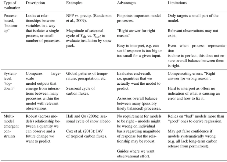
Finally, recommendations for more robust evaluation are discussed. We note that evaluation can be process-based (“bottom-up”) or system-level (“top-down”) (Fig. 1). Evalu-ation can utilise pre-calibrEvalu-ation, and/or emergent constraints across multiple models. A combination of approaches can increase our understanding of a model’s ability to simulate processes across multiple temporal and spatial scales.
Consideration will also be given to how key questions aris-ing in the paper could potentially be resolved through
coor-dinated research activities.
2 The role of data sets in ESM evaluation
ESMs aim to simulate a highly complex system. Non-linearities in the system imply that even a small change in one of the components might unexpectedly influence another component (Roe and Baker, 2007). As such, robust model evaluation is critical to assist in understanding the behaviour of ESMs and the limitations of what we can and cannot rep-resent quantitatively. The development of such approaches to model evaluation requires consideration of many different data types.
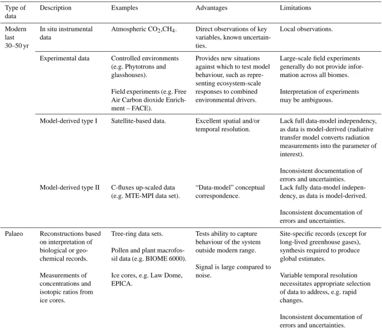
Modern and palaeodata are both used for model eval-uation, although each kind of data has advantages and limitations (Table 1). Experimental data provide bench-marks for a range of carbon cycle-relevant processes (e.g. physiologically-based responses of ecosystems to warming and CO2 increase) that cannot be tested in other
ways. However, for processes that are biome-specific, the limited geographical scope of the relatively few existing records is problematic. Data sets also exist with more global
Fig. 1. Conceptual diagram of hierarchical approach to model eval-uation on different spatial and temporal scales.
coverage, documenting changes in the recent past (last 30– 50 yr), but an inherent limitation of these data sets is that they sample the carbon cycle response to a limited range of varia-tion in atmospheric CO2concentration and climate.
Palaeoclimate evaluation is an important test of how well ESMs reproduce climate changes (e.g. Braconnot et al., 2012). The past does not provide direct analogues for the future, but does offer the opportunity to examine cli-mate changes that are as large as those anticipated dur-ing the 21st century, and to evaluate climate system feed-backs with response times longer than the instrumental pe-riod (e.g. cryosphere, ocean circulation, some components of the carbon cycle).
2.1 Modern data sets
Evaluation analysis can benefit from modern data sets, to test and constrain components within ESMs in a hierarchical ap-proach (Leffelaar, 1990; Wu and David, 2002). Recent ini-tiatives in land and ocean model evaluation and benchmark-ing (land: Randerson et al., 2009; Luo et al., 2012; Kelley et al., 2012; Dalmonech and Zaehle, 2013; ocean: Najjaret al., 2007; Friedrichs et al., 2009; Stow et al., 2009; Bopp et al., 2013) give examples of suitable modern data sets for model evaluation and their use in diagnosing model inconsistencies with respect to behaviour of the carbon cycle. These include instrumental data, such as direct measurements of CO2, and
CH4spanning the last 30–50 yr, measurements from carbon
flux monitoring networks, and satellite-based data of various kinds (Table 1).
Due to their detailed spatial coverage and high temporal resolution, satellite data sets offer the potential to explore the representation of processes in models in detail, and to reveal
Table 1. Summary of key data types for evaluation. Type of
data
Description Examples Advantages Limitations
Modern last 30–50 yr
In situ instrumental data
Atmospheric CO2,CH4. Direct observations of key
variables, known uncertain-ties.
Local observations.
Experimental data Controlled environments (e.g. Phytotrons and glasshouses).
Field experiments (e.g. Free Air Carbon dioxide Enrich-ment – FACE).
Provides new situations against which to test model behaviour, such as repre-senting ecosystem-scale responses to combined environmental drivers.
Large-scale field experiments generally do not provide infor-mation across all biomes. Interpretation of experiments may be ambiguous.
Model-derived type I Satellite-based data. Excellent spatial and/or temporal resolution.
Lack full data-model independency, as data is model-derived (radiative transfer model converts radiation measurements into the parameter of interest).
Inconsistent documentation of errors and uncertainties. Model-derived type II C-fluxes up-scaled data
(e.g. MTE-MPI data set).
“Data-model” conceptual correspondence.
Lack fully data-model indepen-dency, as data is model-derived. Inconsistent documentation of errors and uncertainties. Palaeo Reconstructions based
on interpretation of biological or geo-chemical records. Measurements of concentrations and isotopic ratios from ice cores.
Tree-ring data sets. Pollen and plant macrofos-sil data (e.g. BIOME 6000). Ice cores, e.g. Law Dome, EPICA.
Tests ability to capture behaviour of the system outside modern range. Signal is large compared to noise.
Site-specific records (except for long-lived greenhouse gases), synthesis required to produce global estimates.
Variable temporal resolution necessitates appropriate selection of data to address, e.g. rapid changes.
Inconsistent documentation of errors and uncertainties.
compensating errors in ESMs. One of the main concerns is the lack of full consistency between what we can observe with different satellite sensors (e.g. top of the atmosphere re-flectance) and what models actually simulate (e.g. net pri-mary productivity). The lack of full independence between the data and the model is also an issue that often affects such comparisons. Satellite data are typically model-processed (type 1, Table 1), with some sort of model used to transform the direct measurements of the satellite into other parameters of interest. If, for example, a radiative transfer model is used to estimate the atmospheric or surface state from measured radiances, then there will likely be similarities between the functions used for the retrieval and those used in a climate model. This is not a major problem if the data are used in an
informed way, and indeed it presents opportunities (e.g. the estimated surface variable can be compared with a modelled variable without the model radiative transfer functions being involved). Statistical and change detection retrievals rely not on physical models but on statistical links between variables or on a modulation of the satellite signal. These two types of retrievals sometimes use model data for calibration but are otherwise independent of models. Statistical models in par-ticular are not only useful to evaluate specific parameters in a model, but can also be used to perform process-based eval-uations.
Uncertainty estimates are not always provided or propa-gated during the retrieval process. Nevertheless, modern data sets are a very rich data source with a number of useful
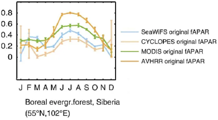
applications. For example, robust spatial and temporal infor-mation emerging from data can be used to rule out unreason-able simulations and diagnose model weaknesses. Satellite-based data sets of vegetation activity depict ecosystem re-sponse to climate variability at seasonal and interannual time scales and return patterns of forced variability that can be useful for model evaluation (Beck et al., 2011; Dahlke et al., 2012), even if bias within the data set is greater than data-model differences (e.g. Fig. 2).
Ecosystem observations, such as eddy covariance mea-surements of CO2 and latent heat exchanges between the
atmosphere and land, and ecosystem manipulation studies, such as drought treatments and free air CO2 enrichment
(FACE) experiments, provide a unique source of informa-tion to evaluate process formulainforma-tions in the land compo-nent of ESMs (Friend et al., 2007; Bonan et al., 2012; de Kauwe et al., 2013). Manipulation experiments (e.g. FACE experiments: Nowak et al., 2004; Ainsworth and Long, 2005; Norby and Zak, 2011) are a particularly powerful test of key processes in ESMs and their constituent components, as shown by Zaehle et al. (2010) in relation to C-N cycle cou-pling, and de Kauwe et al. (2013) for carbon-water cycling. It should be expected that models would be able to repro-duce experimental results involving manipulations of global change drivers such as CO2, temperature, rainfall, and N
ad-dition.
The application of such data for the evaluation of ESMs is challenging because of the limited spatial representativeness of the observations, resulting from the lack of any coherent global strategy for the placement of flux towers or experi-mental sites, and the high costs of running these facilities. Upscaling monitoring data using data-mining techniques and ancillary data, such as remote sensing and climate data, pro-vides one possible means to bridge the gap between the spa-tial scale of observation and ESMs (Jung et al., 2011). How-ever, this can be at the cost of introducing model assump-tions and uncertainties that are difficult to quantify. Further-more, such upscaling is near impossible for ecosystem ma-nipulation experiments, as they are so scarce, and rarely per-formed following a comparable protocol. More and better-coordinated manipulation studies are needed to better con-strain ESM prediction (Batterman and Larsen, 2011; Vicca et al., 2012). Hickler et al. (2008), for example, showed that the LPJ-GUESS model produced quantitatively realistic net primary production (NPP) enhancement due to CO2
eleva-tion in temperate forests, but also showed greatly different responses in boreal and tropical forests, for which no ade-quate manipulation studies exist. These predictions remain to be tested.
The interpretation of experiments is not unambiguous be-cause it is seldom that just one external variable can be al-tered at a time. To give just one recent example, Bauerle et al. (2012) showed that the widely observed decline of Ru-bisco capacity (Vc,max)in leaves during the transition from
summer to autumn could be abated by supplementary
light-Fig. 2. Original fAPAR time series from a selected region (after Dahkle et al., 2012).©American Meteorological Society. Used with permission.
ing designed to maintain the summer photoperiod, and con-cluded that Vc,max is under photoperiodic control, asserting
that models should include this effect. However, their treat-ment also inevitably increased total daily photosynthetically active radiation (PAR) in autumn. On the basis of the infor-mation given about the experimental protocol, these results could therefore also be interpreted as showing that seasonal variations inVc,maxare related to daily total PAR.
This example draws attention to a key principle for the use of experimental results in model evaluation, namely that such comparisons are only valid if the models explicitly follow the experimental protocol. It is not sufficient for models to attempt to reproduce the stated general conclusions of exper-imental studies. The possibility of invalid comparisons can most easily be avoided through the inclusion of experimen-talists from the outset in model evaluation projects. This was the case, for example, in the FACE data-model comparison study of De Kauwe et al. (2013).
This example also illustrates a general challenge for the modelling community. One response to new experimental studies is to increase model complexity by adding new pro-cesses based on the ostensible advances in knowledge. How-ever, we advise a more critical and cautious approach, em-ploying case-by-case comparisons of model results and ex-periments, rather than general interpretation of exex-periments, to reduce the potential for ambiguities and avoid unneces-sary complexity in models. Such an approach would prevent the occurrence of overparameterisation, the implications of which have been explored by Crout et al. (2009).
2.2 Palaeodata
The key purpose of palaeo-evaluation is to establish whether the model has the correct sensitivity for large-scale pro-cesses. Models are typically developed using modern ob-servations (i.e. under a limited range of climate conditions and behaviours), but we need to determine how well they simulate a large climate change, to assess whether they can
capture the behaviour of the system outside the modern range. If our understanding of the physics and biology of the system is correct, models should be able to predict past changes as well as present behaviour.
Reconstructions of global temperature changes over the last 1500 yr (e.g. Mann et al., 2009) are primarily derived from tree-ring and isotopic records, while reconstructions of climates over the last deglaciation and the Holocene (e.g. Davis et al., 2003; Viau et al., 2008; Seppä et al., 2009) are primarily derived from pollen data, although other biotic assemblages and geochemical data have been used at individ-ual sites (e.g. Larocque and Bigler, 2004; Hou et al., 2006; Millet et al., 2009). Marine sediment cores have been used extensively to generate sea-surface temperature reconstruc-tions (e.g. Marcott et al., 2013), and to reconstruct different past climate variables (see review in Henderson, 2002) re-lated to ocean conditions. For example, δ13C is used in re-constructions of ocean circulation, marine productivity, and biosphere carbon storage (Oliver et al., 2010). However, the interpretation of these data is often not straightforward, since the measured indicators are frequently influenced by more than one climatic variable (e.g. the benthic δ18O measured in foraminiferal shells contains information on both global sea level and deep water temperature). Errors associated with the data and their interpretation also need to be stated, as while analytical errors on the measurements are often small, errors in the calibrations used to obtain reconstructions tend to be much bigger. Therefore the incorporation of measured vari-ables such as marine carbonate concentrations (e.g. Ridgwell et al., 2007), δ18O (e.g. Roche et al., 2004) or δ13C (e.g. Cru-cifix, 2005) as variables in models is an important advance, because it allows comparison of model outputs directly with data, rather than relying on a potentially flawed comparison between modelled variables and the same variables recon-structed from chemical or isotopic measurements.
Ice cores provide a polar contribution to climate response reconstruction, as well as crucial information on a range of climate-relevant factors. For example, responses to forcings by solar variability (through10Be), volcanism (through sul-fate spikes), and changes in the atmospheric concentration of greenhouse gases (e.g. CO2, CH4, N2O) and mineral dust
can be assessed. CH4 can be measured in both Greenland
and Antarctic ice cores. CO2measurements require Antarctic
cores, due to the high concentrations of impurities in Green-land samples, which lead to the in situ production of CO2
(Tschumi and Stauffer, 2000; Stauffer et al., 2002). For the last few millennia, choosing sites with the highest snow ac-cumulation rates yields decadal resolution. The highest res-olution records to date are from Law Dome (MacFarling Meure et al., 2006), making these data more reliable, par-ticularly for model evaluation (e.g. Frank et al., 2010). Fur-ther work at high accumulation sites would provide reas-surance on this point. Over longer time periods, sites with progressively lower snow accumulation rates, and therefore lower intrinsic time resolution, have to be used. Through
the Holocene (last ∼ 11 000 yr) (Elsig et al., 2009), and the last deglaciation, i.e. the transition out of the Last Glacial Maximum (LGM) into the Holocene (Lourantou et al., 2010; Schmidt et al., 2012), there are now high-quality13C /12C of CO2data available, as well as much improved information
about the phasing between the change in Antarctic tempera-ture and CO2(Pedro et al., 2012; Parrenin et al., 2013), and
between CO2 and the global mean temperature (Shakun et
al., 2012) .
Compared to the amount of effort spent on reconstructing past climates and atmospheric composition, comparatively few data sets provide information on different components of the terrestrial carbon cycle. Nevertheless, there are data sets – synthesised from many individual published studies – that provide information on changes in vegetation distri-bution (e.g. Prentice et al., 2000; Bigelow et al., 2003; Harri-son and Sanchez Goñi, 2010; Prentice et al., 2011a), biomass burning (Power et al., 2008; Daniau et al., 2012), and peat ac-cumulation (e.g. Yu et al., 2010; Charman et al., 2013). These data sets are important because they can be used to test the response of individual components of ESMs to changes in forcing.
The major advantage of evaluating models using the palae-orecord is that it is possible to focus on times when the sig-nal is large compared to the noise. The change in forcing at the LGM relative to the pre-industrial control is of compa-rable magnitude, though opposite in direction, to the change in forcing from quadrupling CO2relative to that same
con-trol (Izumi et al., 2013). Thus, comparisons of palaeoclimatic simulations and observations since the LGM can provide a measure of individual model performance, discriminate be-tween models, and allow diagnosis of the sources of model error for a range of climate states similar in scope to those ex-pected in the future. For example, Harrison et al. (2013) eval-uated mid-Holocene and LGM simulations from the CMIP5 archive, and from the second phase of the Palaeoclimate Modelling Intercomparison Project (PMIP2), against obser-vational benchmarks, using goodness-of-fit and bias metrics. However, as is the case for many modern observational data sets (e.g. Kelley et al., 2012), not all published palaeorecon-structions provide adequate documentation of errors and un-certainties, and there is a lack of standarisation between data sets where such estimates are provided (e.g. Leduc et al., 2010; Bartlein et al., 2011). Reconstructions based on ice or sediment cores are intrinsically site-specific (except for the globally significant greenhouse gas records), therefore many records are required to synthesise regional or global distri-bution patterns and estimates (Fig. 3). Community efforts to provide high-quality compilations of already available data (e.g., Waelbroeck et al., 2009; Bartlein et al., 2010) make it possible to use palaeodata for model evaluation, but an increase in the coverage of palaeoreconstructions is still re-quired to evaluate model behaviour at regional scales.
Unfortunately, most attempts to compare simulations and reconstructions using palaeodata have focused on purely
Fig. 3. Examples of global data sets documenting environmental conditions during the mid-Holocene (ca. 6000 yr ago) that can be used for benchmarking ESM simulations. In general, these are expressed as anomalies, i.e. the difference between the mid-Holocene and mod-ern conditions: (a) pollen-based reconstructions of anomalies in mean annual temperature, (b) reconstructions of anomalies in sea-surface temperatures based on marine biological and chemical records, (c) pollen and plant macrofossil reconstructions of vegetation during the mid-Holocene, (d) charcoal records of the anomalies in biomass burning, and (e) anomalies of changes in the hydrological cycle based on lake-level records of the balance between precipitation and evaporation (after Harrison and Bartlein, 2012). (Reprinted from Harrison, S. P. and Bartlein, P.: Records from the Past, Lessons for the Future, in: The Future of the World’s Climate, edited by: A. Henderson-Sellars and K. J. McGuffie, 403–436, Copyright©2012, with permission from Elsevier.)
qualitative agreement of simulated and observed spatial patterns (e.g. Otto-Bliesner et al., 2007; Miller et al., 2010). There has been surprisingly little use of metrics for palaeodata-model comparisons (for exceptions see e.g. Guiot et al., 1999; Paul and Schäfer-Neth, 2004; Harrison et al., 2013). This situation probably reflects problems in devel-oping meaningful ways of taking uncertainties into account in these comparisons. Quantitative assessments have gener-ally focused on individual large-scale features of the climate system, for example the magnitude of insolation-induced in-crease in precipitation over northern Africa during the mid-Holocene (Joussaume et al., 1999; Jansen et al., 2007), zonal
cooling in the tropics at the LGM (Otto-Bleisner et al., 2009), or the amplification of cooling over Antarctica relative to the tropical oceans at the LGM (Masson-Delmotte et al., 2006; Braconnot et al., 2012). Comparisons of simulated vegetation changes have been based on assessments of the number of matches to site-based observations from a region (e.g. Harri-son and Prentice, 2003; Wohlfahrt et al., 2004, 2008). Obser-vational uncertainty is represented visually in such compar-isons, and only used explicitly to identify extreme behaviour amongst the models. Nevertheless, the recent trend is towards explicit incorporation of uncertainties and systematic model benchmarking (Harrison et al., 2013; Izumi et al., 2013).
3 Key metrics for ESM evaluation
Many metrics have been proposed (Tables 2–4), and the choice of an appropriate metric in model evaluation is crucial because the use of inappropriate metrics can lead to overcon-fidence in model skill. The choice should be based on the properties of the data sets, the properties of the metric, and the specific objectives of the evaluation. Metric formalism – that is, the treatment of metrics as well-defined mathematical and statistical concepts – can help the interpretation of met-rics, their analysis, or their combination into a “skill-score” (Taylor, 2001) in an objective way.
The use of metrics draws on the mathematical con-cept of “distance” (d(x, y)), expressed in terms of three characteristics: separation: d(x, y) = 0 ←→ x = y, symmetry: d(x, y) = d(y, x), and the triangle inequality
d(x, z)d(x, y) + d(y, z). The two data sets could be two model outputs, where the metric is used to measure how sim-ilar the two models are, or one model output and one refer-ence observation data set, where the metric is used to evaluate the model against real measurements. Three levels of metric complexity can be identified, relating to the state-space on which to apply the distance:
– Level 1 – “comparisons of raw biogeophysical
vari-ables”. Here the distance generally reflects errors and provides assessment of model performance where there is a reasonable degree of similarity between the model and reference data set (such as climate variables in weather models).
– Level 2 – “comparisons of statistics on biogeophysical
variables”. Here the distance is measured on a statisti-cal property of the data sets. This is particularly useful for models that are expected to characterise the statis-tical behaviour of a system (e.g. climate models). This level is appropriate for most of the biophysical vari-ables simulated by ESMs.
– Level 3 – “comparisons of relationships among
bio-geophysical variables”. Here, the distance is diagnos-tic of relationships related to physical and/or biological processes and this level of comparison is therefore use-ful for understanding the behaviour of two data sets.
At all levels of metric complexity, the metric needs to be both synthetic enough to aid in understanding the similari-ties and differences between the two data sets, and to be un-derstandable by non-specialists in order to facilitate its use by other communities. Next, the particular uses, advantages, and limitations of metrics in each level of metric complexity will be discussed.
3.1 Metrics on raw biogeophysical variables
Level 1 metrics are the most widely used. The distance mea-sures the discrepancies between two data sets of a key
bio-geophysical variable. Discrepancies can be measured at site level or at pixel level for gridded data sets, and thus such comparisons can be used for model evaluation against sparse data, such as site-based NPP data (e.g. Zaehle and Friend, 2010), eddy-covariance data (e.g. Blyth et al., 2011), or at-mospheric CO2concentration records at remote monitoring
stations (e.g. Cadule et al., 2010; Dalmonech and Zaehle, 2013). Where there is sufficient data to make the calcula-tion meaningful, comparisons can be made against spatial averages or global means of the biogeophysical variables. Comparisons can also be made in the time domain because climate change and climate variability act on Earth system components across a wide range of temporal scales. The dis-tance can thus be measured on instantaneous variables or on time-averaged variables, such as annual means. Many dis-tances, summarised in Table 2, can be considered to measure these discrepancies.
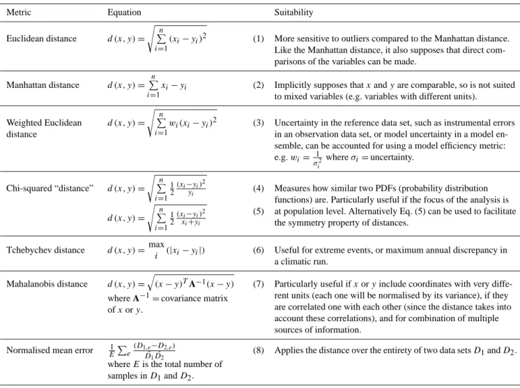
The Euclidean distance (Eq. 1) is the most commonly used distance. It is more sensitive to outliers than the Manhattan distance (Eq. 2). Both of these distances assume that direct comparisons of the data can be made. Some examples are reported in Jolliff et al. (2009), where the Euclidean distance is used to evaluate three ocean surface bio-optical fields.
In the case of the weighted Euclidean distance (Eq. 3), a weight is associated with each variable. This is useful for various reasons: (1) normalisation against a mean value pro-vides a dimensionless metric and allows comparisons to be drawn between data sets with different orders of magnitude; (2) the weighting can take account of uncertainties in the ref-erence data set (e.g. instrumental errors in an observational data set, or uncertainty in a model ensemble); and (3) this type of metric can be useful when the data have a different dynamical range. For example, in a time series of Northern Hemisphere monthly surface temperature, the variability is different for summer and winter, and it makes sense to nor-malise the differences by the variance.
The Chi-square “distance” (Eq. 4) is related to the Pear-son Chi-square test or goodness-of-fit, and differs from previ-ous distances discussed here as it measures the similarity be-tween two probability density functions (PDFs), rather than between data points. It is particularly useful if the focus of the analysis is at the population level. Distances on PDFs are de-fined, in this paper, to be Level 2 metrics, but the Chi-square distance can be used when the geophysical variables are sup-posed to have a particular shape (e.g. an atmospheric profile of temperature). Equation (5) can also be used, in particular to facilitate the symmetry property of distances.
The Tchebychev distance (Eq. 6) can be used, for example, to identify the maximum annual discrepancy in a climatic run. It can be useful if the focus is on extreme events.
The Mahalanobis distance (Eq. 7) is particularly suitable if variables have very different units, as each one will be nor-malised by its variance, and/or if they are correlated with each other, since the distance takes these correlations into ac-count. High correlation between two data sets has no impact
Table 2. Summary of Level 1 metrics (x, y represent points while D1, D2are data sets).
Metric Equation Suitability
Euclidean distance d (x, y) = s
n
P
i=1
(xi−yi)2 (1) More sensitive to outliers compared to the Manhattan distance. Like the Manhattan distance, it also supposes that direct com-parisons of the variables can be made.
Manhattan distance d (x, y) =
n
P
i=1
xi−yi (2) Implicitly supposes that x and y are comparable, so is not suited to mixed variables (e.g. variables with different units).
Weighted Euclidean distance d (x, y) = s n P i=1
wi(xi−yi)2 (3) Uncertainty in the reference data set, such as instrumental errors in an observation data set, or model uncertainty in a model en-semble, can be accounted for using a model efficiency metric: e.g. wi=σ12 i where σi=uncertainty. Chi-squared “distance” d (x, y) = s n P i=1 1 2 (xi−yi)2 yi d (x, y) = s n P i=1 1 2 (xi−yi)2 xi+yi (4) (5)
Measures how similar two PDFs (probability distribution functions) are. Particularly useful if the focus of the analysis is at population level. Alternatively Eq. (5) can be used to facilitate the symmetry property of distances.
Tchebychev distance d (x, y) =max
i (|xi−yi|) (6) Useful for extreme events, or maximum annual discrepancy in
a climatic run. Mahalanobis distance d (x, y) =
q
(x − y)TA−1(x − y)
where A−1=covariance matrix of x or y.
(7) Particularly useful if x or y include coordinates with very diffe-rent units (each one will be normalised by its variance), if they are correlated one with each other (since the distance takes into account these correlations), and for combination of multiple sources of information.
Normalised mean error E1P
e
(D1,e−D2,e) ¯ D1D¯2
where E is the total number of samples in D1and D2.
(8) Applies the distance over the entirety of two data sets D1and D2.
on the distance computed, compared to two independent data sets. This distance is directly related to the quality criterion of the variational assimilation and Bayesian formalism that optimally combines weather forecast and real observations. This criterion needs to take into account the covariance ma-trices and the uncertainties of the state variables.
Interesting links can be established between metrics and the operational developments of the numerical weather pre-diction centres. The Mahalanobis distance is well suited for Gaussian distributions (meaning here that the data/model misfit distribution follows a Gaussian distribution with co-variance matrix A, e.g. Min and Hense, 2007). General Bayesian formalism can be used to generalise this distance to more complex distributions. The Mahalanobis distance and the more general Bayesian framework are particularly suit-able to treat several evaluation issues at once, such as the quantification of multiple sources of error and uncertainty in models or the combination of multiple sources of information (including the acquisition of new information). For instance, Rowlands et al. (2012) use a goodness-of-fit statistic similar
to the Mahalanobis distance applied to surface temperature data sets.
We present here distances between two points, possibly multivariate. Some metrics use these distances and have been defined over the two whole data sets D1and D2. For
exam-ple, the Normalized Mean Error (NME) is a normalisation of the bias between the two data sets (Eq. 8). Several other distances exist in the literature that have been applied in dif-ferent scientific fields and that are not listed here (e.g. Deza and Deza, 2006). However most of these distances are par-ticular cases or an extension of the preceding distances.
3.2 Metrics on statistical properties
Level 2 metrics, summarised in Table 3, use statistical quan-tities estimated for two data sets D1 and D2. Some of the
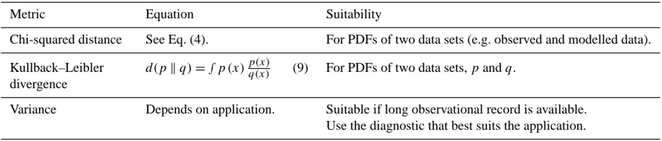
metrics presented in the previous section can then be applied to the selected statistics. For instance, the PDF can be es-timated for both data sets and the Chi-Square distance can be used to measure their discrepancy. For example, Anav et al. (2013) compared the PDFs of gross primary production
Table 3. Summary of Level 2 metrics.
Metric Equation Suitability
Chi-squared distance See Eq. (4). For PDFs of two data sets (e.g. observed and modelled data). Kullback–Leibler
divergence
d(p k q) = ∫ p (x)p(x)q(x) (9) For PDFs of two data sets, p and q.
Variance Depends on application. Suitable if long observational record is available. Use the diagnostic that best suits the application.
(GPP) and leaf area index (LAI) from the CMIP5 model sim-ulations with two selected data sets.
The Kullback–Leibler divergence (Eq. 9) is based on in-formation theory and can also be used to measure the simi-larity of two PDFs. The Kolmogorov–Smirnov distance can be used when it is of interest to measure the maximum dif-ference between the cumulative distributions. Tchebychev or other distances acting on estimated seasons are also consid-ered here to be Level 2 metrics, since the seasons are statis-tical quantities estimated on D1and D2(although very close
to level 1 raw geophysical variables). Similarly the distance can operate on derived variables from the original time se-ries as decomposed signals in the frequency domain. Cadule et al. (2010), for example, analysed model performance in terms of representing the long-term trend and the seasonal signal of the atmospheric CO2record.
The variance of data and model is often used to formulate metrics for the quantification of the data-model similarity. In coupled systems, the use of a metric based on distance can become inadequate; the metric no longer facilitates def-inite conclusions on the model error, because it includes an unknown parameter in the form of the unforced variability. Furthermore, when applied to spatial fields, as variance is strongly location-dependent, a global spatial variance can be misleading. Gleckler et al. (2008) proposed a more suitable model variability index which has been applied to climatic variables, but is also highly applicable to several of the bio-geophysical and biogeochemical variables simulated by land and ocean coupled models, and thus relevant to the carbon cycle. The metric can also focus on extreme events, with the distance acting on the percentile, assuming that the length of the records is sufficient to characterise these extremes.
3.3 Metrics on relationships
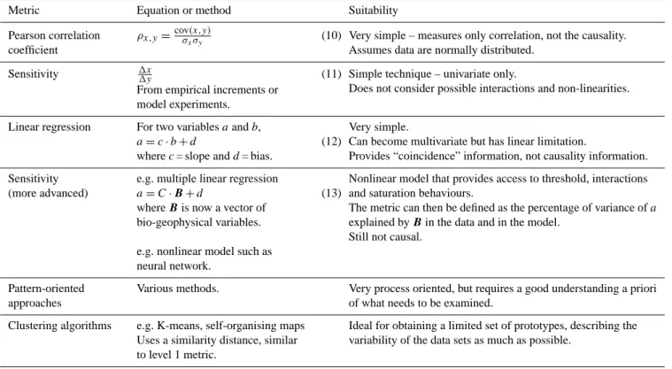
Level 3 metrics, summarised in Table 4, focus on relation-ships. The aim here is to diagnose a physical or a biophys-ical process that is particularly important, such as the link between two variables in the climate system. Various “rela-tionship diagnostics” have been used, and are summarised in Table 4.
The correlation between two variables is a very simple and widely used metric; it satisfies the need to compare the
data-model phase correspondence of a particular biogeophysical variable. In this case parametric statistics such as the Pear-son correlation coefficient (Eq. 10), or non-parametric statis-tics such as the Spearman correlation coefficient, are directly used as a metric. This is particularly used to evaluate the cor-respondence of the mean seasonal cycle of several variables, from precipitation (Taylor, 2001), to LAI, GPP (Anav et al., 2013), and atmospheric CO2(Dalmonech and Zaehle, 2013).
The sensitivity of one variable to another can be estimated using simple to very complex techniques (Aires and Rossow, 2003). It can be obtained by dividing concomitant perturba-tions of the two variables using spatial or temporal differ-ences (Eq. 11), or by perturbing a model and measuring the impact when reaching equilibrium. The first approach can be used to evaluate, for example, site-level manipulative exper-iments to estimate carbon sensitivity to soil temperature or nitrogen deposition in terrestrial ecosystem models (e.g. Luo et al., 2012).
From the linear regression of two variables the slope or bias can be compared for D1 or D2 (Eq. 12). The slope is
very close to the concept of sensitivity, but sensitivities are very dependent on the way they are measured. For example, sensitivity of the atmospheric CO2 to climatic fluctuations
may depend on the timescales they are calculated on (Cadule et al., 2010). An alternative, when more than two variables are involved in the physical or biophysical relationship under study, is a multiple linear regression (Eq. 13), or any other linear or nonlinear regression model such as neural networks. See, for example, the results obtained at site-level by Moffat et al. (2010).
Pattern-oriented approaches use graphs to identify partic-ular patterns in the data set. These graphs aim at capturing relationships of more than two variables. For example, in Bony and Dufresne (2005), the tropical circulation is first decomposed into dynamical regimes using mid-tropospheric vertical velocity and then the sensitivity of the cloud forcing to a change in local sea surface temperature (SST) is exam-ined for each dynamical regime. Moise and Delage (2011) proposed a metric that assesses the similarity of field struc-ture of rainfall over the South Pacific Convergence Zone in terms of errors in replacement, rotation, volume, and pat-tern. The same metric could be applied to ocean Sea-viewing Wide Field-of-view Sensor (SeaWiFS) satellite-based fields
Table 4. Summary of Level 3 metrics.
Metric Equation or method Suitability
Pearson correlation coefficient
ρx,y=cov(x,y)σxσy (10) Very simple – measures only correlation, not the causality. Assumes data are normally distributed.
Sensitivity 1x1y
From empirical increments or model experiments.
(11) Simple technique – univariate only.
Does not consider possible interactions and non-linearities.
Linear regression For two variables a and b,
a = c · b + d
where c = slope and d = bias.
(12)
Very simple.
Can become multivariate but has linear limitation.
Provides “coincidence” information, not causality information. Sensitivity
(more advanced)
e.g. multiple linear regression
a = C ·B + d
where B is now a vector of bio-geophysical variables. e.g. nonlinear model such as neural network.
(13)
Nonlinear model that provides access to threshold, interactions and saturation behaviours.
The metric can then be defined as the percentage of variance of a explained by B in the data and in the model.
Still not causal.
Pattern-oriented approaches
Various methods. Very process oriented, but requires a good understanding a priori of what needs to be examined.
Clustering algorithms e.g. K-means, self-organising maps Uses a similarity distance, similar to level 1 metric.
Ideal for obtaining a limited set of prototypes, describing the variability of the data sets as much as possible.
in areas where particular spatial structures emerge. These powerful techniques could be more widely applied to eval-uating ESM processes.
Clustering algorithms have been used to obtain weather regimes based only on the samples of a data set. For ex-ample, Jakob and Tselioudis (2003) and Chéruy and Aires (2009) obtained cloud regimes based on cloud properties (optical thickness, cloud top pressure). The same methodol-ogy can be used in D1and D2and the two sets of regimes
can be compared. The regimes can also be obtained on one data set and only the regime frequencies of the two data sets are compared. Abramowitz and Gupta (2008) applied a distance metric to compare several density functions of modelled net ecosystem exchange (NEE) clustered using the “self-organising map” technique.
It is often difficult to use a real mathematical distance to measure the discrepancy between the two “relationship di-agnostics”. Although very useful for understanding differ-ences in the physical behaviour, the simple comparison of two graphs (for D1and D2)is not entirely satisfactory since
it does not allow combination of multiple metrics or defini-tion of scoring systems. In this paper, it is not possible to list all the ways to define a rigorous distance on each one of the relationship diagnostics that have been presented: Eu-clidean distance can be used on the regression parameters or the sensitivity coefficients, or two weather regime frequen-cies can be measured using confusion matrices (e.g. Aires et al., 2011). The distance needs to be adapted to the
rela-tionship diagnostic. The most limiting factor to this type of approach for ESM evaluation is that the relationship obtained might be not robust enough (i.e. statistically significant), or not easily framed within a process-based context.
4 A framework for robust model evaluation
Robust model evaluation relies on a combination of ap-proaches, each informed using appropriate data and metrics (Fig. 4). Calibration and, ideally, pre-calibration (Sect. 4.2.2) must first be employed to rule out implausible outcomes, us-ing data independent of that which may be subsequently used in model evaluation. Then, evaluation approaches must be a combination of process-focussed and system-wide, to ensure that both the representation of processes and the balance be-tween them are realistic in the model. Optionally, the results of different model evaluation tests can be combined into a single model score, perhaps for the purposes of weighting future projections. When employed as part of a multi-model ensemble, the simulation can also contribute to the calcula-tion of emergent constraints, which can then be used in sub-sequent model development (Sect. 4.3.3).
4.1 Recommendations for improved data availability and usage
The increasingly data-rich environment is both an opportu-nity and a challenge, in that it offers more opportunities for
Fig. 4. Schematic diagram of model evaluation approaches, with optional approaches indicated by dashed lines.
model validation but requires more knowledge about the gen-eration of data sets and their uncertainties in order to de-termine the best data set for evaluation of specific process representations. While improved documentation of data sets would go some way to alleviating the latter problem, there is scope for improved collaboration between the modelling and observational communities to develop an appropriate bench-marking system, that evolves to reflect new model devel-opments (such as representing ecosystem-scale responses to combined environmental drivers) not addressed by existing benchmarks.
4.1.1 Coordinating data collection efforts
A key question for both the modelling and data communi-ties to address together is how well model evaluation re-quirements and data availability are reconciled. There is an ongoing need for new and better data sets for model eval-uation: data sets that are appropriately documented and for which useful information about errors and uncertainties are provided. The temporal and spatial coverage of data sets also needs to be sufficient to capture potential climatic pertur-bations, a point that is illustrated in the evaluation of ma-rine productivity. Modelling studies offer conflicting evi-dence of the behaviour of this key variable in controlling marine carbon fluxes and exchanges of carbon with the at-mosphere under a changing climate (e.g. Sarmiento et al., 2004; Steinacher et al., 2010; Taucher et al., 2012; Laufkötter et al., 2013), therefore model evaluation is essential. Recent compilations of observations of marine-productivity proxies give us a reasonably well-documented picture of qualitative changes in productivity over the last glacial-interglacial tran-sition (e.g. Kohfeld et al., 2005), and in response to Heinrich events (e.g. Mariotti et al., 2012). These data sets are being used to evaluate the same ESMs used to predict changes in NPP in response to climate change (e.g. Bopp et al., 2003; Mariotti et al., 2012), and these studies show reasonable
agreement. On more recent timescales, remote sensing ob-servations of ocean colour have been used to infer decadal changes in marine NPP. Studies show an increase in the ex-tent of oligotrophic gyres over 1997–2008 with the SeaWiFS data (Polovina et al., 2008). However, on longer timescales, and using Coastal Zone Color Scanner (CZCS) and SeaWiFS data sets, analysis yields contrasting results of increase or de-crease of NPP from 1979–1985 to 1998–2002 (Gregg et al., 2003; Antoine et al., 2005). Henson et al. (2010) have shown, based on a statistical analysis of biogeochemical model out-puts, that an NPP time series of ∼ 40 yr is needed to detect any global-warming-induced changes in NPP, highlighting the need for continued, focused data collection efforts.
4.1.2 Maximising the usefulness of current data in modelling studies
Modelling studies should be designed in a manner that makes the best use of the available data. For example, equilibrium model simulations of the distant past require time-slice re-constructions for evaluating processes relating to the car-bon cycle. These reconstructions rely on synchronisation of records from ice cores, marine sediments, and terrestrial se-quences, to take account of differences between forcings and responses in different archives, which is a significant effort even within a particular palaeo-archive, let alone across mul-tiple archives. Yet the strength of palaeodata is precisely that it offers information about rates of change, and such informa-tion is discarded in a time-slice simulainforma-tion. For that reason, the increasing use of transient model runs to simulate past climate and environmental changes is a particularly impor-tant development.
There is also an increasing need for forward modelling to simulate the quantities that are actually measured, such as isotopes in ice cores and pollen abundances. Ice core gas con-centration measurements are unusual because what is mea-sured is what we want to know, and is a variable that ESMs yield as a direct output. This is not generally the case, nor are all model setups easily able to simulate even the trace-gas isotopic data that are available from ice. A corollary is that we need to recognise the difficulty of trying to use palaeo-data to reconstruct quantities that are essentially model con-structs, for example inferring the strength of the meridional overturning circulation (MOC) from the231Pa /230Th ratio in marine sediment cores (McManus et al., 2004). In the latter context, direct simulation of the231Pa /230Th ratio is neces-sary to deconvolute the multiple competing processes (Sid-dall et al., 2005, 2007).
4.1.3 Using data availability to inform model development
Model development should also focus on incorporating pro-cesses that, at least collectively, are constrained by a wealth of data. Notable examples are processes such as those
governing methane (CH4) emissions (e.g. from wetlands and
permafrost) and the removal of methane from the atmosphere (e.g. via oxidation by the hydroxyl radical and atomic chlo-rine). There are four main observational constraints on the CH4 budget with which we can evaluate the performance
of ESMs: the concentration, [CH4]; its isotopic
composi-tion with respect to carbon and deuterium, δ13CH4and δD
(CH4); and CH4fluxes at measurement sites. We have no
nat-ural record of CH4fluxes so their use in ESM evaluation is
limited to the relatively recent period in which they have been measured, though measurements of CH4 fluxes at specific
sites can be used to verify spatial and seasonal distributions of CH4emissions inferred from tall tower and satellite
mea-surements of [CH4], by inverse modelling. However, a range
of [CH4], δ13CH4, and δD (CH4) records are available,
span-ning up to 800 000 yr in the case of polar ice cores, which can be used to evaluate the ability of ESMs to capture changes to the CH4budget in response to past changes in climate. The
variety of climatic changes we can probe, from large glacial-interglacial changes spanning thousands of years to substan-tial changes over just a few tens of years at the beginning of Dansgaard–Oeschger events, and still more rapid, subtle changes following volcanic eruptions, enables us to evaluate the ability of ESMs to capture both the observed size and speed of changes known to have taken place. The comple-mentary natures of the [CH4], δ13CH4, and δD (CH4)
con-straints is key to ESM evaluation. Each CH4source and sink
affects these three constraints in different ways. As such, sce-narios that explain only one set of observations can be elimi-nated. For instance, an increase in CH4emissions from
trop-ical wetlands, biomass burning, or methane hydrates could explain an increase in [CH4], but of these only an increase in
biomass burning emissions could explain an accompanying enrichment in δ13CH4. Of course, more than one factor can
change at a time, but the key point is that the most rigorous test of ESM performance utilises all three constraints and, therefore, ESMs should track the influence of each source and sink.
4.2 Recommendations for model calibration 4.2.1 Key principles of model calibration
Model evaluation is closely linked to model calibration. ESMs contain a large number of (sometimes poorly con-strained) parameters, resulting from incomplete knowledge of certain processes or from the simplification of complex processes, which can be calibrated in order to improve model behaviour. In general, model calibration should fol-low a number of fundamental guiding principles. The prin-ciples detailed here are mostly based on the discussion in Petoukhov et al. (2000) for the CLIMBER-2 model.
First, parameters which are well constrained from obser-vations or from theory must not be used for model calibra-tion. Normally it would be physically inappropriate to
mod-ify the values of fundamental constants, for example, or use a value for a parameter which is different from the accepted empirical measurement just to improve the performance of the model.
Second, whenever possible, parameterisations and sub-modules should be tuned separately against observations rather than in the coupled system. In the case of parame-terisations, this ensures that they represent the physical be-haviour of the process described rather than their effect on the coupled system. The same principle should be applied as far as possible to the individual sub-modules of any ESM to make sure that their behaviour is self-consistent and to fa-cilitate calibration of the much more complex fully coupled system.
Third, parameters must describe physical processes rather than unexplained differences between geographic regions. It is preferable for the model to represent the physical be-haviour of the system rather than apply hidden flux correc-tions.
Fourth, the number of tuning parameters must be smaller than the predicted degrees of freedom. However, this is usu-ally large for ESMs.
Finally, one of the key challenges relating to data used in ESM evaluation is to what extent ESM development and evaluation data are independent. In principle, the same ob-servational data should not be used for calibration and eval-uation. This is difficult to enforce in practice, however. Even if the observational data are divided into two parts, with one part used for calibration and the other for evaluation, for ex-ample, any mismatch in the evaluation will likely lead to a readjustment of model tuning parameters, making the evalu-ation not completely independent of the calibrevalu-ation proce-dure (Oreskes et al., 1994). Standard leave-one-out cross-validation techniques divide calibration data sets into mul-tiple subsets, sequentially testing the calibration on each left-out subset (in the limit each data point) in turn but in Earth system modelling the subsets are unlikely to be fully inde-pendent.
4.2.2 Utilising pre-calibration to constrain implausible outcomes
The essence of pre-calibration is to apply weak constraints to model inputs in the initial ensemble design, and weak con-straints on the model outputs to rule out implausible regions of input and output spaces (Edwards et al., 2011).
The pre-calibration approach is based on relatively sim-ple statistical modelling tools and robust scientific judge-ments, but avoids the formidable challenges of applying full Bayesian calibration to a complex model (Rougier, 2007). A large set of model experiments sampling the variability in multiple input parameter values with the full simulator, here the ESM, is used to derive a statistical surrogate model or “emulator” of the dependence of key model outputs on un-certain model inputs. The choice of sampling points must be
highly efficient to span the input space and is usually based on Latin hypercube designs. The resulting emulator is com-putationally many orders of magnitude faster than the orig-inal model and can therefore be used for extensive, multi-dimensional sensitivity analyses to understand the behaviour of the model. Holden et al. (2010, 2013a, b) demonstrated the approach in constraining glacial and future terrestrial carbon storage.
The process is usually iterative, in that a large proportion of the initial parameter space may be deemed implausible, but one or more subsequent simulated ensembles can be de-signed by rejection sampling from the emulator to locate the not-implausible region of parameter space. The result-ing simulated ensembles are then used to refine the emulator and the definition of the implausible space. The final output is an emulator of model behaviour and an ensemble of sim-ulations, corresponding to a subset of parameter space that is deemed “plausible” in the sense that simulations from the identified parameter region do not disagree with a set of ob-servational metrics by more than is deemed reasonable for the given simulator. The level of agreement is therefore de-pendent on the model and represents an assessment of the expected magnitude of its structural error (i.e. error due to choices for how processes are represented and relate to one another). The plausible ensemble, however, is a general re-sult for the model that can be applied to any relevant predic-tion problems, and embodies an estimate of the structural and parametric error inherent in the model predictions.
Ideally, pre-calibration is a first step in a full Bayesian cal-ibration analysis. The advantage of the logistic mapping or pure rejection sampling approach used is that, because no weighting is applied, a subsequent Bayesian calibration can be applied to refine the evaluation without any need to un-ravel convolution effects or the multiple use of constraints. In practice, however, the pre-calibration step can be suffi-cient to extract all the information that is readily available from top-down constraints given the magnitude of uncertain-ties in inputs and of structural errors in intermediate com-plexity ESMs.
4.3 Recommendations for model evaluation methodologies
4.3.1 Process-based (bottom-up) evaluation
Both bottom-up and top-down evaluation are required for evaluating ESMs: the first approach can give process-by-process information but not the balance between them; the second will give the balance but not the single terms. When bottom-up, process-based improvements can be shown to have top-down, system-level benefits, then we know our multi-pronged evaluation has worked.
Bottom-up, process-based evaluation will often require combinations of data to create the appropriate metrics as it is more likely to focus on the sensitivity of one output
vari-able to changes in a single input. For example, to assess if a model has the right sensitivity of NPP to precipitation a test could be to compute the partial derivative of NPP with respect to precipitation at constant values of temperature, ra-diation etc. for both the model and the observations (Rander-son et al., 2009). This approach requires processing a data set of, in this case, NPP, to combine it with precipitation data to derive a relationship. The same NPP data could be com-bined with temperature data to derive a similar NPP(T ) rela-tionship. This is much more likely to isolate at least a small number of processes than simply comparing simulated NPP to a observational map or time series.
It is also common for model development to focus on spe-cific features or aspects of the model in order to have faith in the model’s ability to make projections. For example, climate modelling centres may focus on the ability of their GCMs to represent coupled phenomena such as ENSO, or the timing and intensity of monsoon systems. In this way, bottom-up evaluation pinpoints important model processes, and helps to confirm that the model is a sufficiently accurate representa-tion of the real system, giving the right results for the right reasons. However, a key limitation of this approach is that the relevant observations needed to assess a particular pro-cess may not exist.
Process-based evaluation requires metrics based on process-based sensitivities, as described in Sect. 3.2. Sensi-tivity analysis (e.g. Saltelli et al., 2000; Zaehle et al., 2005) may be useful to determine the parameters and processes to focus on in a bottom-up evaluation. In this approach, a sim-ple statistical model is used to represent the physical relation-ships in the reference data set. A similar model is calibrated on the model simulations and the complex multivariate and non-linear relationships can then be compared.
Measuring these sensitivities allows prioritisation of the important parameters to validate in the model and isolate pro-cesses not well simulated in the model. For example, Aires et al. (2013) used neural networks to develop a reliable statis-tical model for the analysis of land–atmosphere interactions over the continental US in the North American Regional Re-analysis (NARR) data set. Such sensitivity analyses enable identification of key factors in the system and in this exam-ple, characterisation of rainfall frequency and intensity ac-cording to three factors: cloud triggering potential, low-level humidity deficit, and evaporative fraction.
4.3.2 System-level (top-down) evaluation
Top-down constraints tend to focus on whole-system be-haviour and are more likely to involve evaluation of spa-tial or time-series data. Typical quantities used for top-down evaluations include surface temperature, pressure, precipi-tation, and wind speed maps. Observational data sets exist for many of these quantities throughout the atmosphere, so zonal-mean, or 3-dimensional comparisons are also possible (Randall et al., 2007). Anav et al. (2013) extend this approach