Mission planning

HAL Id: hal-01318418

https://hal.archives-ouvertes.fr/hal-01318418

HAL is a multi-disciplinary open access archive for the deposit and dissemination of sci-entific research documents, whether they are pub-lished or not. The documents may come from teaching and research institutions in France or abroad, or from public or private research centers.

L’archive ouverte pluridisciplinaire HAL, est destinée au dépôt et à la diffusion de documents scientifiques de niveau recherche, publiés ou non, émanant des établissements d’enseignement et de recherche français ou étrangers, des laboratoires publics ou privés.

Mission planning

Maria Joao Rendas

To cite this version:

Maria Joao Rendas. Mission planning. [Research Report] D5.5.2, Laboratoire d’Informatique, Sig-naux, et Systèmes Sophia Antipolis, CNRS UNS. 2016. �hal-01318418�

[CHAPTER 3 OF DELIVERABLE D5.5.2 OF PROJECT DRONIC

]

March 2016

MISSION PLANNING

The planning remote service is responsible for defining the trajectories of the vehicles before mission execution. It is logically a component of the DSS and interacts only with other DSS components, as specified in deliverable D1.1.3. A more constrained version of the server software is also included in the Adaptive Guidance module see D2.2.3, for re-planning the nominal mission plan after periods of adaptive sampling.

DRONIC missions can involve: (a) only the Master vehicle (when the goal is to acquire a map of some environmental field), (b) only the Slave vehicle (when a treatment mission is to be defined based on a prior hot-spot map) or (c) both (simultaneous map and treatment). This section is organized in the following manner. We start by describing the protocol for interaction with the planning server (section 4.1). Section 4.2 is dedicated to the planning of mission maps, presenting the two geometric planners that have been implemented in DRONIC, while section 4.3 addresses planning of the treatment missions, which strongly relies on the geometric planners presented in section 4.2. Finally, section 4.4 summarizes the main outcomes and conclusions.

1.1 Planning server

The DSS can obtain a mission plan by remotely calling the application I3S.MissionPlan().

I3S.MissionPlan(MissionFile, [PlanMethod,] [PriorModel,] )

MissionFile is the name of a Mission File following the format specifications indicated in Annex B of D1.1.3 (v11, 07/12/015 ). Note that the two last parameters are optional.

In particular the following fields of the Mission File are important:

MissionType : indicates the type of mission to be planned

• map : pre-programmed mapping mission (involving only the Master vehicle) • adap : adaptive mapping mission (involving only the Master vehicle)

• treat : treatment mission (involving only the Slave vehicle)

• map&treat : mapping and treatment mission (using both vehicles)

• adap&treat : adaptive mapping and treatment mission (using both vehicles)

SiteName : name of the water body. Optional.

LaunchPoint : geographic (latitude, longitude) location of the launching point for the

mission.

RecoveryPoint : geographic location of recovery point. If missing, it will be set equal to the

launching point.

BoundingBox : list of geographic positions delimiting the zone to be mapped.

ForbiddenZones : list of forbidden zones, each one a list of points (fields lat,long) indicating

zones that the vehicle(s) should not enter. Optional.

Bloom : this field is required only for missions of type adap, map&treat or adap&treat, and

defines the condition that indicates the zones to be treated (and/or actively searched for in the case mapping is involved). It has fields Bloom.Sensor and Bloom.Value. Regions with values of the indicated sensor above the specified threshold will be actively mapped and/or treated.

Master_speed , Slave_speed: default vehicle(s) speed. Optional (a default value of 1 m/s is

used for the master and 0.5 m/s for the slave, if not specified otherwise).

Master_length, Slave_length : maximum trajectory lengths (a default value of 20 km is used

for the master and 15 km for the slave, if not specified otherwise).

Safety: a safety distance from border (shores).

Minimal_spatial_rate: a minimal value of the distance between segments of the vehicle path.

Calling this application will produce a complete Mission File with the same name (the old one will be over-written), containing the field Master_Path (and Slave_Path for missions involving treatment), that defines the nominal trajectory of the platform(s). We stress that even for adaptive missions a nominal plan must be defined for the Master vehicle.

PlanMethod is a string that indicates the planning algorithm to be used. For the moment the following are near final implementation (updates of this deliverable will be produced for each new releases of the server, in particular if new planning methods are added).

• Transect : this choice will cover the region by a series of linear transects linking the launching and end points

• SpaceFillingCurve (the default setting). Produces a curved line filling the indicated region linking the launching and recovery points.

PriorModel is the name of a file containing information extracted from historical data or from outputs of mathematical models of the observed field. For treatment only missions, this is be name of a file describing the contours of the hot-spots that must be treated, see section

Erreur ! Source du renvoi introuvable..

Note: at the moment this report is written, we do not have sufficient data about the algae

fields to enable a precise definition of the format of this file, and how it will be generated in the context of DRONIC. However, we preferred to consider it from start in the specification of the interface, in an effort to minimize the need for future modifications.

1.2 Planning mapping missions

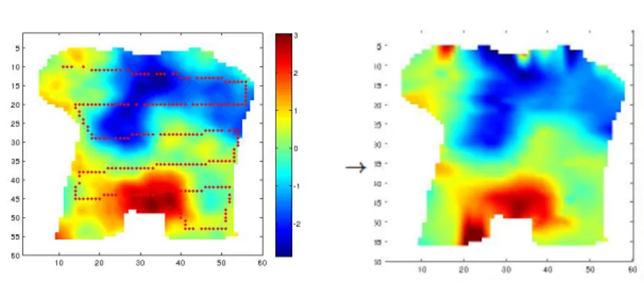
Figure 1: Surveying.

The goal of mapping (surveying) is to gather a set of measures from which a representation of

the variation of some field f(.) over a given region A can be extracted, as shown in the above

Figure.

In DRONIC, the available data is a set of point measures taken by the robotic platform (the Master vehicle) along a path P, illustrated in the Figure by the red dots in the left plot.

Let Ξ be the set of sampled positions (the “design”) and let f(Ξ) denote the values measured at the sampled locations. We assume that some algorithm F (the interpolation algorithms used in DRONIC have been presented in D5.5.1) is able to extrapolate the set of geo-localized measured (Ξ, f(Ξ)) at any point :

.

We are not be concerned in this document with the choice of F, but rather with the choice of the path P along which the measures are to be taken:

Ξ = ξ1,…,ξN, ξk = P(lk).

where {lk} is a regular sampling of curve P, at a fixed spatial rate (we assume the vehicle

speed is constant and the sensor sampling rate is fixed). Note that the spatial sampling rate is not a design variable, and all we can choose is the trajectory P. To stress this dependency of

the design Ξ in the curve P we use the notation .

Ideally, P is chosen such that some criterion of discrepancy D between the true and reconstructed fields is minimized, i.e., solving the problem  

Solving this problem without constraints on P leads to an infinite length space filling curve inside A, everywhere dense in A, which is not a plan realizable by a real robot in finite time and energy. We must thus consider constrained solutions of the problem above. The natural constraint is the one that expresses the power limitations of the platform, and that can be easily transformed into a limitation of the total length L of P:

Since the true field is unknown the criterion above cannot be computed. Two approaches

are then possible:

1. Spread the set of measures as uniformly as possible in A. This approach is

implicitly based on the hypothesis that the larger the distance from s to the

for the observed field , like isotropy and spatial stationarity, this uniformity criterion is related to minimizing the maximum reconstruction error.

2. Assume some stochastic model for is known. Then minimization of the actual

error for each observation can be replaced by the minimization of its expected (average) value under the assumed distribution.

As it has already been stated, implementation of design algorithms that optimized the

expected value of some discrepancy between true field and the reconstructed map, that require

knowledge of a probabilistic model for the observed field, has not yet been possible in DRONIC.

Waiting that these datasets are made available, which will then allow the identification of relevant models for the locations where the DRONIC system will be operated, only approach 1 above has been implemented in the DRONIC mission-planning server. The next sections describe the methods retained in the project.

1.2.1 Planning mapping missions using geometric criteria

Choosing points where to make measurements so that a given criterion is optimized is known in the scientific literature as the “experimental design problem”.

A classical criterion, of a purely geometric nature, goes under the name of “space filling”. While the meaning of what space filling is seems quite intuitive (a set of measurement sites that evenly covers the domain A), its mathematical formulation is not obvious, and several distinct “space filling” criteria have been proposed in the scientific literature. We present below some common “space filling” criteria, assuming that a metric structure is defined over

A – in the case of DRONIC this is simply a closed subset of the 2D Euclidean space. Denote

by its boundary (usually composed of several connected components).

! MaxMin. This “worst-case” criterion measures the distance between closest pairs of sampled points, whose minimum value should be as large as possible. This is formally a sphere covering problem – see FigureFigure 2 The sphere covering problem (reprinted from Mathworld) – where we search for the maximal radius r of N circles with center in A that completely cover region A (the circles’ centers are the design points). Note that this criterion tends to define designs which are regular grids, putting some points in the boundary of A. Note that the complexity of computing this criterion depends only on the design size N, but not on the area/volume of A.

Figure 2 The sphere covering problem (reprinted from Mathworld)

! MinMax. This criterion is apparently very similar to the previous one: it measures the distance between a generic point of A to the closest design point, whose maximum value (over the point of A considered) should be minimized. This is equivalent to a

non-intersecting circles that can be contained in A, see FigureFigure 3 for an illustration. Contrary to MaxMim, this criterion does put design points in the boundary of A (since pushing design points at the boundary inside the region A necessarily results in a lower value of the MinMax criterion). This criterion can be related to moments of the interpolation error under a set of restrictive assumptions, and is considered to be

preferable to MaxMin, but the high complexity associated to its computation (which

grows with the size of A) limits its effective practical utilization.

! We note that being, as MaxMin, a “worst-case” criterion, MinMax also tends to produce designs where several points of A are at the MinMax distance of the closest sampled point.

Figure 3 Sphere packing (reprinted from http://www.grasshopper3d.com/)

! Entropy/Discrepancy criteria. A significant number of alternative criteria have been proposed in the experimental design literature, motivated by interpreting the design as a realization of a stochastic spatial process. A common one is Discrepancy, that can be related to the Kolomogorov test of equality between the empirical distribution of the number of points falling in a given family of compact sets to the distribution is induced in the same sets by the uniform spatial Poisson process. Discrepancy measuring, in this sense, distance to uniformity, it should be as small as possible. This criterion has been extensively studied for sequences filling the unit hyper-cube of Euclidean spaces, resulting in the definition of several families of “low-discrepancy” (Sobol, Alton,…). In our work in DRONIC we rely on the existence of these sequences to identify trajectories P that are space-filling curves, but for regions with more generic geometry than the classical hypercube. The reader is refered to [??] for a presentation of statistically based space filling criteria.

Our work in the context of DRONIC departs in some aspects of the framework classically considered in experimental design:

1. Our design points are not “free”: they must be a regular sample of some continuous path P.

2. The number N of points of the design, which is usually consider to be fixed, must replaced in our setting by a bound on the total length L=|P| of the robot trajectory P. 3. We must depart from simplistic assumptions about the geometry of A like the unit

hyper-cube prevailing most experimental design studies. In our case A is an arbitrary bounded region of the 2D space, not convex and possibly with holes (islands).

Under these modified constraints, our goal is still to find a design that “uniformly covers A”. More precisely, our goal is to try to approximate the optimal MinMax solution, and thus minimize the maximum distance of the points of A to the vehicle’s path P, keeping its length not larger than L.

1.2.1.1 Boustrophédon paths

The equivalence of the MinMax and MaxMin “space filling” criteria to sphere packing and sphere covering problems, respectively, highlights their relation to the robotic “complete covering path” problem, where the goal is to find a minimal length path P inside a closed subset A of the Euclidean space such that its dilation (in the sense of the mathematical morphology operators) by some compact set B completely covers A.

Note that in the robotic framework set B is usually dictated by the actual platform (e.g. the footprint of some tools in cleaning or the range of some observation sensor – e.g. sonar — in inspection problems) and its size is fixed. In DRONIC, the size of B is unknown, and must be chosen as the smallest one such that the resulting covering path has length not larger than the pre-specified L.

The coverage path problem has been studied by many authors in the framework of mobile robotics. A classical solution has been proposed by [Choset] that presented an algorithm that covers the target region with a series of parallel transects that “uniformly” cover the region of interest (while avoiding obstacles or other forbidden zones). Note the similarity to the surveying trajectories customary in environmental surveys.

Since the pioneering work of Choset, a number of variants have been proposed, in particular in two directions: (i) find a complete coverage path “on-line”, i.e., at the same time as a map of A is learnt; (ii) find optimal solutions, instead of just “good” ones. In the planning server of DRONIC we are concerned with planning mapping missions for a known water body, and thus “on-line” planning methods are not relevant.

The now classic Boustrophédon algorithm – and all its many variants – partition a bounded region into a number of adjacent cells that can be covered with a simple polygonal path, consisting of a series of parallel transects not further than a given distance apart (this distance is related to the size of the set B above). This decomposition, which has been shown to be formally related to the sets defined by the interplay of the level sets of some Morse function and the boundary , and is based on the identification of the set of critical points of ,

which are the points at which the normal to the level lines of the Morse function is collinear

with the normal at . Most commonly, in the 2 dimensional plan with generic point s=(x,y)

the Morse function chosen is simply one of the coordinates of a local Cartesian frame (e.g.

f(x,y) = x), and the critical points are the singular points of (x). Note that since A can have

holes (islands, or non accessible regions), its boundary can have several connected components (the contour of the water body and the contours of all the islands present inside

A).

A planning tool using this approach is available through the DRONIC mission-planning server. It solves the following problem:

! Given a specification of the boundary of A (a list of points describing each connected

component), a starting/end point and a total length L;

! it finds a non self-intersecting closed path P completely contained in A passing

through , of length not larger than L, that is a list alternating local

See Figure 6 for a typical mission plan generated by this planner. This planner integrates a number of software modules:

1. A compression algorithm that simplifies the description of the coast lines received from the user. This algorithm (IfShades, for incremental fuzzy shape description) has been proposed [RendasRolfes] in the context of simultaneous localisation and mapping for mobile robots with no access to GPS-like position information (like underwater robots, or platforms working in some in-doors configurations), and linearly scans a list of points defining a contour while producing an approximation as a series of “fuzzy lines”.

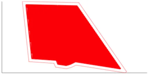
The goal of this first step is to reduce the numerical complexity of the planning problem, related to the complexity of the contours’ geometry (more precisely to its number of critical points, see below). Figure 4 Simplified polygonal approximation of a water body contour by algorithm IfShades.shows the result of processing a water body contour by IfShades .

The input of this step is the collection of contours Ck , k=1,…,K describing ,

each one a list of points: Ck = (sk,1,…s_k,Nk). Its output is a collection of simpler

contour descriptions, C’k = (pk,1,…p_k,Mk), with, in general, Mk << Nk.

Furthermore, a “dilated” (in the sense of mathematical morphology operators) version of these simplified contours is computed, to prevent the planned path to

get closer to the than the safety distance δ (the original and dilated contours are

visible in Figure 4, the black curve being the dilated version of the original contours shown in green) indicated in the Mission File. Note that δ is held constant and is not equal to the distance between the parallel transects that compose the final trajectory, which is in general different.

Note that in this step some contours can be merged (their dilated versions intersect).

Figure 4 Simplified polygonal approximation of a water body contour by algorithm IfShades.

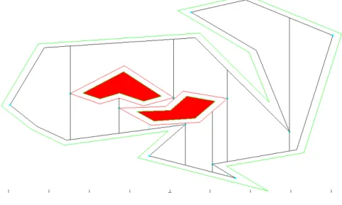
2. Geometric analysis of the polygonal contour, identifying the critical points and the partition of A into a set of cells topologically equivalent to a trapezoid, which can be easily covered by a Boustrophédon path (one example is shown in Figure 5, where the black vertical lines indicate the limits of the cellular decomposition).

The Reeb graph G=(V,E), whose nodes (V) are the critical points of and the

arcs represent the cells of the partition of A, is built in this step.

Once the cellular decomposition is found the total area of A can be easily

computed, leading to an initial value on the spacing Δ between linear transects

of the final path.

The input of this step are the simplified contour descriptions C’k, defining the free

space of A, and its output is the Reeb graph G defining the cellular decomposition of A.

Figure 5 Decomposition of a region in trapezoidal-like cells.

3. Determination of an edge-covering circuit for graph G. This problem is known in graph theory as the Chinese Postman problem (CPP), and several algorithms have been proposed to solve it in an optimal manner, in particular minimizing the number of arcs that must be crossed twice. The algorithms proposed in these references are optimal. Unfortunately, their complete description is very complex and hard to find.

More importantly, the optimality criterion considered (the number of arcs crossed twice) is not relevant to our planning problem (what is relevant for us is the length of the over-head of a “come-&-go” path in a cell with respect to a simple path going across the cell), we decided to design and implement a new algorithm to solve it. Note that this algorithm uses extensively the information about the

position and type of the critical points of , and does not solve the generic CPP

problem.

The paths found by our algorithm satisfy a strong constraint on their orientation, enabling us later (in step 5 below) to design locally a Boustrophédon path covering

each cell, while still guaranteeing that the global path is simple (i.e., that it has no self-intersections).

The input to this step is the Reeb graph found in the previous step. Its output is a

(clockwise) list Q=(E1,…,EL) defining the order by which the edges of G must be

crossed, and that contains at least once every edge of G. Note that several edges of the Reeb graph may appear more than once in Q.

4. Length constraint satisfaction. Q and G allows the computation of the total length of the resulting path, and we can thus if required update line spacing parameter Δ such that the constraint on total length is satisfied (see below).

5. Finally, we determine the way-points of a simple closed curve (the final robot mission plan) that covers the cellular regions with a series of parallel linear transects with the computed line spacing Δ, visiting them in the order specified by

Q. This step relies strongly on the constrains that have been imposed to circuit Q

in step 3.

An example of the result is shown in Figure 6. The algorithm scans linearly the list

Q, working locally in each region (corresponding to an element Ei of the list L),

and deciding when (a) to effectively cover the region with a series of parallel transects, (b) whether to leave (or not) space – close to a part of – for an second passage through the region, (c) when to directly go across the region – through the region left unexplored –, or (d) to directly jump to one adjacent cells above/below.

Figure 6 Example of simple space filling (Boustrophédon) curve.

The following is a pseudo-code of the complete operations of the planning server

1. Read the input Mission File and extract the contour, launching/recovery point and length, safety and sampling rate information;

2. Run the algorithm IfShades and dilate its result by the safety distance to obtain a simplified description of the free space (contour merging may occur in this step); 3. Compute the Reeb graph G

4. Identify the circuit Q

5. Compute an initial value of Δ based on the total area and maximum allowable path length

Δ = Area/Maximum Length;

6. Simplify the circuit Q by dropping the elements of the Reeb Graph that are too narrow for the current level of detail (Δ).

7. Find the nominal path by filling each cell of G by the order specified by Q with a Boustrophédon path.

8. Check that the length of the produced path satisfies the maximum length constraint. Presently we accept paths within 5% of the total indicated length. This can be easily changed if the user partners of DRONIC prefer another behaviour). Otherwise Δ is modified using the ratio between the current value of Δ and the ratio of area to path length or, equivalently:

Δnew = Maximum length.

If Δ is modified steps 6 and 7 are repeated.

9. Produce a complete version of the received Mission File, with of the vehicle trajectory (Master_path field).

The code is completely coded in C/C++. It is undergoing final testing before deployment in the planning server.

The next section presents the results obtained for a series of test Mission Files received from VITO in the beginning of March.

1.2.1.2 Test examples

All plans are formapping missions, where the goal is to cover as evenly as possible the region delimited by the specified outer boundary (field InBox in the Mission file).

We point out that the current version of the software addresses the case where launching and recovery points coincide. In that case any point along the boundary can be connected to the closed non-intersecting path that is designed by the application.

Note that the for coincident (or very close) Launching and Recovery Points the initial point can be anywhere in the Inbox contour.

Test site Peyrolles

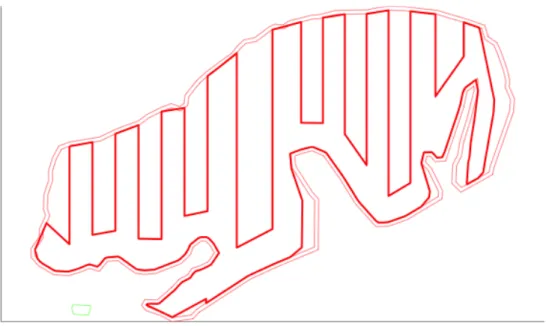
Figure 7 Mission using the maximum allowable path length (20 Kms).

This examples shows that we should set a minimum limit to the inter-line spacing, otherwise for small regions like this one we get a (not useful) very dense sampling.

The same mission with a maximum path length of 10 Kms:

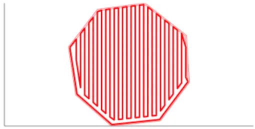
Figure 8 Mssion for maximum path length equal to 10 kms (Δ= 6.26 m). MissionFile 2 (one obstacle)

Figure 9 Mission with the presence of an obstacle. Maximum allowable length equal to 10 Kms (Δ= 3.96 m).

Note that the obstacle close to the lakeshore has been merged with the exterior contour in the dilation step.

Test site Gavervijver

Figure 10: No obstacles. Maximum Length 20 Km, actual path length 20.107 Km.

The size of this region is much larger, and its shape much more complex than the previous case. Note that in the regions not wide enough to make a series of parallel lines the contour goes through the middle of the region (see e.g. the peninsula in the South-East part of the lake).

Figure 11: Same site as above, but for a maximum length of 10 Km.

This Figure (as well as the next one) shows that when the interline spacing becomes very large (i.e. for very small path lengths with respect to the total area to be covered) the variation of interline spacing along the design can be significant (with larger concentration in the regions of smaller width).

Figure 12: Large inter-line spacing may induce an important variation when there are narrow regions.

Mission site Bankart

Site Blankaart

Figure 15: One long obstacle touching the outside contour. Maximum Length 20 Kms, actual length: 18.176 Kms.

Several improvements of the current work are under-way.

! One concerns the treatment of narrow regions and passages inside A, for which a decision must be taken of whether to drop their coverage or to make a single passage near their centre (skeleton of the corresponding region). This subject deserves a detailed discussion with our end-user partners and those that are responsible for modelling, to adopt a solution that suits their specific needs.

! A more profound one concerns the optimality of the simple closed edge-covering curve found in step 3 above. Our current algorithm is iterative: it starts by computing the longest possible clockwise closed circuit going through the cells whose boundary intersects the lake boundary (note that such a circuit always exists). Then it iteratively augments this circuit by adding an edge not in the circuit (a “come & go “ path covering one of the edges of the Reeb graph). The position of the existing closed circuit where the new edges are inserted is determined such that the global clockwise consistency of the direction of the circuit (i.e., from left to right and from top to bottom) is maintained. Being iterative (in some sense, “greedy”) our current algorithm may fail to find the simplest solutions, in particular circular motions around inner-most islands that may be possible. With Prof. Fédou are currently studying a recursive version of the algorithm, based on the coding of the regions geometry by a Dyck word, and hope to be able soon to release a more efficient solution to step 2.

1.2.1.3 Direct optimisation: TSP on a cluster of points using a GA

The geometry of the trajectories produced by the planner presented in the previous section is strongly constrained. More importantly, the resulting design (the set of discrete points along

the vehicle’s trajectory at which samples will be taken) has a preferred sampling direction (the direction of the vertical lines), along which the behaviour of the field is much better sampled than along all other spatial directions. This may induce spurious artefacts in the interpolated field. For this reason, we studied the problem of finding less constrained space filling curves than Boustrophédon paths.

One (conceptually) simple manner of generating a space filling closed curve inside A, is to rely on the existence of good discrete space filling designs in the unit hyper-cube, like the Alton or Sobol sequences. Let W be the smallest hypercube containing area A and sn, n=1

,…,K>>1 be a space filling sequence in W. Since the “space filling” property is a local

property, we can obtain a space filling sequence {s’n} in A by eliminating all points {sn} that

are not inside A. The size of this set does not significantly impacts the final result.

A closed curve with good space filling properties can then be created by solving a Travelling

Salesman Circuit (TSC) problem on the graph with nodes {s’n} and edge weights equal to the

length of the shortest between the corresponding nodes completely contained in A. Solving

the TSC problem directly in the low discrepancy sequence {s’n} is usually too heavy, and that

a more manageable problem is obtained by performing clustering of the points {s’n} in a much

smaller number of points.

Although many solutions are openly available for solving the TSC problem, we found that the existence of islands and the non-convexity of A easily leas to paths not entirely covered in A, and for this reason we dropped this approach and defined a new one presented in the next section.

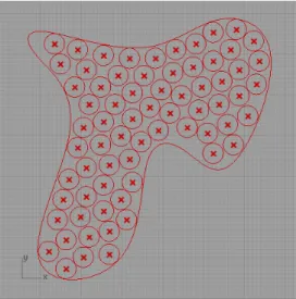
1.2.1.4 Exploitation of the properties of Kohonen networks

Kohonen networks, also called Self-Organising Feature Maps (SOFM) have been proposed in the 80’s as a computational structure able to capture the geometry of the support of a given distribution, by filling it with a series of points on which a system of neighbourhoods is defined.

SOFMs are in this manner able to learn the interdependency of a set of variables. Note the important role played by the system of neighbourhoods defining the topological relation between the nodes of the network. Figure 16: Bi-dimensional Kohonen network (reprinted

from http://www.mathworks.com/matlabcentral) shows the response of a 10 by 10 square

SOFM to a sequence of points drawn from the uniform distribution in after some

iterations of the learning algorithm, demonstrating the ability of uniformly spreading the network’s nodes in the unit rectangle. In fact, it has been shown [cite] that for networks of large size, and a topology compatible with the distance in the embedding linear space, the Kohonen network converges - asymptotically in the number of data points – to a state where the density of network nodes inside a set C is proportional to the cubic-root of the probability that the input points fall in C.

Figure 16: Bi-dimensional Kohonen network

Our smooth solution to the space filing curve problem is based on this property of SOFMs: we update the state of a SOFM with a convenient topology with points uniformly drawn inside A. Note that since we work with the uniform distribution, we are insensitive to the fact that the density of the map’s nodes will replicate the cubic-root of the generating distribution. Drawing points uniformly in an connected region of arbitrary geometry, which can be non-convex and with holes, is not a trivial task. We rely on the Reeb decompostion of A presented in the section 3.2.1.1, randomly selecting a cell of the cellular decomposition, and then drawing uniformly inside the cell. To do this, we start by generating a low-discrepancy sequence in the unit rectangle that covers each of the cells (see previous section). Two points are then randomly selected from the sequence associated to the cell, and a point is drawn at random as a convex linear combination of the selected points (note that by construction the convex combination always is inside the cell). We can in this manner define an infinite sequence of inputs sk, k=1,2,… that will used to drive the state of the SOFM (its node’s

positions).

For the SOFM to be defined, we further need to impose a system of neighbourhoods in the network nodes xn, n=1,…,N. Since we want to find a closed circuit, we establish a circular

linear topology, node n being adjacent to the previous (mod(n-1,N)+1) and next (mod(n,N)+1) nodes.

After convergence, the positions of the nodes of the SOFM can be used directly as way-points, defining a piece-wise linear trajectory inside A. Alternatively, they can be smoothed using any universal interpolator like cubic splines. Since in DRONIC, ultimately, the vehicle trajectory is always a piece-wise path, defined by the sequence of way-points specified in the Mission File, we directly use the nodes of the SOFM as the way-points of the nominal mission.

The length of the trajectories generated by the SOFM is related to the number of network nodes (N) and is not easily controlled. The algorithm currently implemented, and that will soon be integrated in the planning server, proceeds by iterative steps of refinement and decimation.

Traditionally, the SOFM is initialized from a random state, the position of each node being drawn at random in some set that must intersect A. The initial state of our SOFM also exploits the Reeb decomposition of A, i.e. the graph G, as well as the CPP circuit Q. The nodes of the

network are partitioned in the distinct cells, with the number of points nk associated to cell k

being equal to the ration of the cell’s region to the area of A. The nk points of each cell are

sequentially selected from the low discrepancy sequence in Ck. Finally, for all adjacent cells in Q, a pair of nodes in the corresponding sequences is chosen and linked to the sequence of points of the neighbouring cells. This initialization exploits the ability of the Reeb graph to capture the geometry of A.

This tailored initialisation only offers faster convergence of the SOFM, but also help bias the paths produced. Figure 17 Paths produced by SOFM. shows examples of the resulting paths. Remark much less rigid geometry of these trajectories compared to the Boustrophédon paths, as well as the dependency of the resulting path length on the number of nodes of the SOFM network.

1. Read the input Mission File and extract the contour, launching/recovery point and length information;

2. Run the algorithm IfShades and dilate its result to obtain a simplified description of the free space;

3. Compute the Reeb graph G

4. Identify the circuit Q

5. Define the low discrepancy sequences in each cell of G and initialize the state of an SOFM with K nodes;

6. Update until convergence the state of the network drawing uniformly in the support of

A (using the low discrepancy sequences computed in step 5).

7. Compute the length L of the resulting path and adjust the size of the network by dichotomy: if L is larger than the specified limit, reduce the network size by sub-sampling the current path, if L is smaller than the allowable length, increase the number of nodes of the SOFM by over-sampling the current path. In both cases return to step 6.

8. Produce a complete version of the received Mission File, that contains the information of the vehicle trajectory.

This processing flow shares a number of elements with the one presented in section 3.2.1.1, introducing some new software components, for steps 5, 6 and 7. At present, the corresponding modules are coded in Matlab.