HAL Id: insu-03066334
https://hal-insu.archives-ouvertes.fr/insu-03066334
Submitted on 15 Dec 2020
HAL is a multi-disciplinary open access
archive for the deposit and dissemination of
sci-entific research documents, whether they are
pub-lished or not. The documents may come from
teaching and research institutions in France or
abroad, or from public or private research centers.
L’archive ouverte pluridisciplinaire HAL, est
destinée au dépôt et à la diffusion de documents
scientifiques de niveau recherche, publiés ou non,
émanant des établissements d’enseignement et de
recherche français ou étrangers, des laboratoires
publics ou privés.
To cite this version:
Sarah Albertin, Joël Savarino, Slimane Bekki, Albane Barbero, Nicolas Caillon. Measurement report:
Nitrogen isotopes (δ15N) and first quantification of oxygen isotope anomalies (∆17O, δ18O) in
at-mospheric nitrogen dioxide. Atat-mospheric Chemistry and Physics Discussions, European Geosciences
Union, 2021, pp.(Under Review). �10.5194/acp-2020-1143�. �insu-03066334�
Measurement report :
Nitrogen isotopes (δ
15
N) and first
quantification of oxygen isotope anomalies (Δ
17
O, δ
18
O) in
atmospheric nitrogen dioxide
Sarah Albertin
1,2, Joël Savarino
2, Slimane Bekki
1,Albane Barbero
2and Nicolas Caillon
21LATMOS/IPSL, Sorbonne Université, UVSQ, CNRS, 75005 Paris, France
5
2IGE,Univ. Grenoble Alpes, CNRS, IRD, Grenoble INP, 38000 Grenoble, France
Correspondence to: Sarah Albertin (sarah.albertin@latmos.ipsl.fr)
Abstract. The isotopic composition of nitrogen and oxygen in nitrogen dioxide (NO2) potentially carries a wealth of
information about the dynamics of the nitrogen oxides (NOx = nitric oxide(NO) + NO2) chemistry in the atmosphere. While
nitrogen isotopes of NO2 are subtle indicators of emissions, NOx chemistry and isotopic nitrogen exchange between NO and
10
NO2, oxygen isotopes are believed to reflect only the O3/NOx/VOC chemical regime in different atmospheric environments.
In order to access this potential tracer of the tropospheric chemistry, we have developed an efficient active method to trap atmospheric NO2 on denuder tubes and measured, for the first time, its multi-isotopic composition (δ15N, δ18O, and Δ17O). The
δ15N values of NO
2 trapped at our site in Grenoble, France, show little variability (−11.8 to −4.9 ‰) with negligible N isotope
fractionations between NO and NO2 due to high NO2/NOx ratios. NOx emissions main sources are estimated using a stable
15
isotope model indicating the predominance of traffic NOx emissions in this area. The Δ17O values, however, reveal an important
diurnal cycle peaking in late morning at (39.2 ± 1.7) ‰ and decreasing at night until (20.5 ± 1.7) ‰. On top of this diurnal cycle, Δ17O also has substantial variability during the day (from 29.7 to 39.2 ‰), certainly driven by changes in the O
3 to
peroxyl radicals ratio. The night-time decay of Δ17O(NO
2) appears to be driven by NO2 slow removal, mostly from conversion
into N2O5, and its formation from the reaction between O3 and emitted NO. Our Δ17O(NO2) measured towards the end of the
20
night is quantitatively consistent with typical values of Δ17O(O
3). These preliminary results are very promising for using Δ17O
of NO2 as a probe of the atmospheric oxidative activity and for interpreting NO3− isotopic composition records.
1 Introduction
Nitrogen oxides (NOx = NO2 + NO) are at the heart of tropospheric chemistry, as they are involved in key reaction chains
governing the production and destruction of compounds of fundamental interest for health, ecosystems and climate issues 25
(Brown, 2006; Finlayson-Pitts and Pitts, 2000; Jacob, 1999). For example, NO2 photolysis followed by reaction of NO with
peroxy radicals (RO2 = HO2 + RO2) is the only significant source of ozone (O3) in the troposphere where it serves as a severe
air pollutant and a greenhouse gas. Tropospheric O3 also plays a major role in the production processes of radicals which are
responsible for the oxidation and removal of compounds emitted into the atmosphere (Crutzen, 1996). This “cleaning” ability is referred to as the atmospheric oxidative capacity (AOC; Prinn, 2003). Additionally, NOx species are at the core of the
30
acidification and eutrophication (Galloway et al., 2004) and aerosol radiative forcing (Liao and Seinfeld, 2005). In order to better understand the reactive nitrogen (which includes NOx and HNO3) chemistry and the related AOC, it is necessary to
better constrain individual chemical processes driving NOx chemistry.
Stable isotopes analysis is a powerful tool for tracing emissions sources, the individual chemical processes and budgets of 35
atmospheric trace gases (Kaye, 1987). Because different processes favour lighter or heavier isotopologues, the isotopic composition of a chemical species will often vary according to the specific physico-chemical and biological processes it has undergone. This phenomenon of isotopic fractionation can thus be used to trace different processes involved in the formation of the chemical species being analyzed. Isotopic enrichment (δ) of an element X is expressed in ‰ and defined as: δnX =
(nR
spl/nRref − 1) with nR the elemental isotope abundance ratio of the heavy isotope over the light isotope (e.g. for oxygen
40
isotopes 18R(18O/16O) ≡ 18R = x(18O)/x(16O) or 17R(17O/16O) ≡ 17R = x(17O)/x(16O), with x the isotopic abundance) in a sample
(Rspl) and in a reference (Rref). The Vienna Standard Mean Ocean Water (VSMOW; Li et al., 1988) and atmospheric nitrogen
(N2; Mariotti, 1984) are the international references for oxygen and nitrogen ratios, respectively. Most natural isotopic
fractionations are mass dependent fractionations (MDF; Urey, 1947), as it is notably the case for terrestrial oxygenated species in which the triple oxygen composition follows δ17O 0.52 × δ18O (Thiemens, 1999). Yet, laboratory experiments (Thiemens
45
and Heidenreich, 1983) and atmospheric observations (Johnston and Thiemens, 1997; Krankowsky et al., 1995; Vicars and Savarino, 2014) have showed that the isotopic composition of ozone formed in the atmosphere does not follow this canonical MDF relationship and reflects mass independent fractionation (MIF) processes. The important deviation from the MDF oxygen relationship is called the oxygen-17 anomaly (Δ17O) and is defined here in its approximate linearized form as Δ17O = δ17O −
0.52 × δ18O. Our choice of this linear definition is mainly motivated by its convenience for mass balance calculations and its
50
validity for our large Δ17O values and variability. Overall, biases related to our choice of the linear definition are marginal in
our conditions (Assonov and Brenninkmeijer, 2005). It follows that Δ17O inherited from ozone can be considered as conserved
during MDF processes.
The multi-isotopic composition of NOx is therefore a very valuable tracer of its emissions and chemistry in the atmosphere.
However, so far, Δ17O of atmospheric NO
2 (Δ17O(NO2)) has been investigated only using laboratory (Michalski et al., 2014)
55
and modelling (Alexander et al., 2009, 2020; Lyons, 2001; Morin et al., 2011) approaches with theoretical frameworks, and these results need to be tested against atmospheric observations. Walters et al. (2018) have presented a method of sampling and analysing nitrogen ang oxygen stable isotopes of NO2 collected separately at daytime and nighttime in an urban area but
they did not report on Δ17O. Dahal and Hastings (2016) have attempted to measure Δ17O of NO
2 collected on passive samplers,
but the isotopic signal was partly degraded during the sampling and the analytical procedures. Building on their work, we 60
present here an efficient method to collect atmospheric NO2 for isotopic analysis and present the first measurements of triple
oxygen isotopes and double nitrogen isotopes of atmospheric NO2. After estimating the nitrogen isotopic fractionation between
NO and NO2, we infer from δ15N of the NO2 (δ15N(NO2)) the major emissions sources of NOx influencing our sampling site
to investigate the links between the variability of the oxygen isotope anomaly of NO2 and its formation pathways. We also
65
revisit the Morin et al. (2011) NOx isotopic theoretical framework and extend it to urban environments.
2 Materials and Methods
2.1 Sampling method
NO2 was sampled on an active (pumped) collection system using denuder tubes. This method is more efficient to collect NO2
than passive methods (Røyset, 1998), allowing for shorter collection times with a breakthrough of the absorption capacity 70
below 1 %. (Buttini et al., 1987; Williams and Grosjean, 1990). The sampled air was pumped through a ChemCombTM 3500
speciation cartridge (Thermo ScientificTM, USA). Initially used for the speciation of gases and aerosols, these advanced
sampling platforms consist of a PM2.5 impactor inlet connected to a stainless-steel cylinder that contains two glass honeycomb
denuders connected in series for gas collection and a Teflon stage filter pack for aerosols. To collect NO2, glass tubes were
coated with an alkaline guaiacol solution. In basic medium, guaiacol (IUPAC name: 2-Methoxyphenol) is known to react with 75
NO2 to form stable NO2− ions (Nash, 1970) that preserve the original NO2 isotopic signal due to the basic nature of the medium
(pH = 14 after 10 ml extraction). Because NO or peroxyacetyl nitrate (PAN) are not collected by guaiacol, this methodology avoids potential interference from these compounds in later analyses (Buttini et al., 1987). Although nitrous acid (HONO) can bind as NO2−, it is unlikely to adversely impact the results as its concentration is much lower than NO2 (by a factor of 10 to
20) even in very polluted cities (Harris et al., 1982). 80
To evaluate the sampling system performance, a series of experiments were run with artificial gaseous NO2. Using a
commercial gas standard generator (KinTek FlexStreamTM) feed with zero-air, artificial NO
2 (Metronics DynacalTM) was sent
through a ChemComb cartridge while NOx concentration was measured up- and down-stream of the cartridge. From 1 to 30
nmol mol-1 of NO
2 (representative of rural to urban atmospheric conditions), concentrations coming out of the cartridge were
never above the noise level of the NOx monitor (2.5 nmol mol−1). To estimate the denuders trapping efficiency, we passed
85
different concentrations of gaseous NO2 through the collection apparatus and measured the amount of NO2− collected on the
two denuders both connected in series. The denuder efficiency E was then calculated according to the following equation (Buttini et al., 1987):
𝐸 = (1 −𝑏
𝑎 ) × 100 % (1)
with a and b representing the amount of NO2− collected on the first and the second denuder, respectively. From 0.3 to 1.3 µmol
90
of NO2 generated (see Fig. 1), the mean E value was about (97 ± 3) %. The amount of NO2− measured on second denuders
were reproducible and equivalent to blanks, representing on average 3 % of the quantity measured on the first denuders. In light of these results, denuders in second position were not subjected to isotopic analysis and allowed trapping efficiency control.
95
100
105
2.2 Isotopic analysis
Simultaneous isotopic analyses of δ15N, δ18O, and δ17O were performed using a FinniganTM-MAT253 isotope ratio mass
spectrometer (IRMS) following techniques described by Casciotti et al. (2002) and Kaiser et al. (2007). The azide method (McIlvin and Altabet, 2005) was used where 100 nmol of nitrites was converted to N2O using a 50:50 by volume mixture of
110
2M sodium azide and 100 % acetic acid. The principle of identical treatment (Brand, 1996) was strictly respected where the standards and samples possessed the same nitrite concentration, water isotopes, total volume and matrix. Three international KNO2 salts standards, RSIL-N7373, RSIL-N10219, and RSIL-N23 with respective δ15N/δ18O values of –79.6/4.2 ‰, 2.8/88.5
‰, and 3.7/11.4 ‰ were used for normalisation of δ-scale. Scale contraction factors were obtained with the linear regression between measured and known values of δ15N and δ18O. Although the three standards cover a wide range of isotopic
115
composition in δ15N and δ18O, they do not have an isotopic anomaly in 17O. For δ17O-scale, MDF fractionation slope (0.52) is
assumed for two of these laboratory-prepared nitrite standards (see Appendix A for more details). Accuracy of this analytical method on δ17O, δ18O and δ15N measurements was estimated as the standard deviation (σ) of the residuals between our
measurements of the RSIL standards and their expected values. Additionally, isotopic integrity from denuders extraction to the analysis by IRMS has been investigated and showed no degradation over several weeks (see Appendix B) confirming that 120
this method is suitable for isotopic analysis of NO2, as first demonstrated by Walters et al. (2018). The uncertainties applied
to our measurements of δ15N, δ17O and δ18O are reported as the propagation error of the measurement uncertainty and the
uncertainty resulting from sample storage. Uncertainty on Δ17O is derived from the propagation error of the overall uncertainty
on δ17O and δ18O. In our study, average uncertainties on δ15N, δ17O, δ18O, and Δ17O are estimated to be ± 0.1, ± 1.1, ± 2.5 and
± 1.7 ‰, respectively (1σ uncertainties). 125
Figure 1: Correlation plot of NO2 collected on the first
denuder tube of the sampling cartridge vs. NO2 produced by
2.3 Study site and atmospheric NO2 collection
Atmospheric NO2 was collected at the Université Grenoble Alpes campus site. Located to the eastern Grenoble urban area
(690 000 inhabitants), the campus stands between a major transportation route and the Isère river. The city is located at the confluence of three valleys surrounded by mountain chains that influence the atmospheric dynamics and the local air quality. During winter, persistent temperature inversions combined with intense domestic heating can lead to severe PM10 pollution
130
events (Largeron and Staquet, 2016) with daily-average concentration above World Health Organisation thresholds. In summer, emissions are mainly controlled by road traffic that can result in heightened ozone concentrations, especially during stagnant conditions.
Sampling was conducted on a platform five meters above the ground surface. Ambient air was drawn through the cartridge with a Millipore vacuum pump at a flow rate of 10 L min−1(room temperature and one atmospheric pressure) adjusted using a 135
Cole-ParmerTM flowmeter (accuracy ± 3 %). Samples were collected during 24 hours with 3 h sampling intervals during the
day and 5 h sampling from midnight to 5:00 am in order to capture the daily variability in NO2 isotopic composition. Ambient
NO and NO2 concentrations were measured with a 2B TechnologiesTM NO monitor model 410 paired with a NO2 converter
model 401.
Honeycomb denuders were cleaned and coated the day before sampling. After being generously rinsed (5 minutes under a 140
stream of deionised water), the denuders were placed in a vacuum chamber (Thermo ScientificTM Refrigerated VaporTrap
paired with a SpeedVac Concentrator) and dried at 40 °C during 1 hour. Then, denuders internal walls were individually coated with 10 ml of a 95:5 by volume mixture of 2.5 M KOH (prepared in methanol) and ultrapure guaiacol prepared daily. Denuders were then drawn off, dried in the vacuum chamber at 40 °C during 30 minutes to minimize blanks, hermetically sealed and stored at ambient temperature in the dark until usage. The different components of the cartridge (impactor, filters, denuders) 145
were cleaned, dried and fitted together just before use. At the end of the sampling period both denuders were removed from the ChemComb cartridge and rinsed with 10 ml of deionised water in order to leach trapped NO2 out. 1 ml of the eluent was
rapidly used to determine the nitrite concentration using the Griess-Saltzman reaction and UV-vis spectrometry at 520 nm. Recovered eluent ( 7 ml by denuder) was poured in a labelled 15 ml corning® and stored in a freezer until isotopic analysis
the following days. 150
3 Atmospheric observations and multi-isotopic measurements
3.1 NOx and O3 atmospheric observations
Figure 2 shows the time evolution of the hourly NO2, NO and O3 mixing ratio measured during the period covering two nights
and one day (from 15 May 2019 21:00 to 16 May 2019 5:00). Note that most of our NO measurements are found to be within the reported detection limit of the instrument except in the morning (see Table 1) and therefore have to be treated with lot of 155
agreement with the range of values measured at the local air quality site located a kilometre south of the sampling site (https://www.atmo-auvergnerhonealpes.fr/).
During both nights, most of the NOx are in the form of NO2. After sunrise, there is rapid interconversion between NO and
NO2, driven by NO2 photolysis and reactions of NO with O3 and peroxy radicals (Jacob, 1999). NO2 levels are maximum on
160
15 May between 4:00 and 10:00 with a sharp peak of 19 nmol mol−1 at 8:00. After the morning rise, NO2 decreases to reach a
background concentration of about (2.7 ± 0.2) nmol mol-1. This diurnal variation is common in urban/suburban sites
characterised by a morning peak caused by important NOx emissions, mainly from road traffic (Mayer, 1999). As morning
progresses, the boundary layer height increases rapidly, favouring fast dilution of NOx concentrations. Moreover, during the
day, NO2 is converted to HNO3, notably by its reaction with OH radicals. Thus, NOx concentration remains low during the day
165
likely because of the combination of atmospheric dilution by vertical mixing and efficient chemical conversion by OH and organic radicals (Tie et al., 2007). In dense urban areas, a second NOx traffic emission peak can occur in late afternoon but it
is not observed at our sampling site for that specific day. This surface pollution peak is usually weaker than the morning peak due to an elevated boundary layer and a wider period of evening commute. After sunset, NO2 concentrations increase gently
and reach a smooth peak with a maximum of 11 nmol mol−1 around 1:00 am local time, also recorded at the local air quality 170
site. This NO2 concentration rise may be due to low NO emissions (converted to NO2 by reaction with O3) combined with a
decreasing boundary layer height during the night which traps atmospheric species close to the surface (Tie et al., 2007; Villena et al., 2011).
Ozone also exhibits a diurnal variation typical of urban areas (Velasco et al., 2008). O3 peaks around 50 nmol mol−1 at the
beginning of both nights to then declines continuously. Indeed, after sunset, O3 production ceases and its concentration drops
175
due to its dry deposition, reactions with organics, and O3 titration by NO emitted from evening traffic, heating, and industrial
activities in the stable nocturnal boundary layer (Klein et al., 2019). O3 reaches a minimum (about 15 nmol mol−1) not at the
end of the night but during the morning rush hours peak of NO. Ox (= O3 + NO2) is a more conservative quantity than O3
because it is less affected by conversion of O3 into NO2 through NO titration which is important in urban environments
(Kleinman et al., 2002). For instance, between 6:00 and 8:00 am, O3 is strongly titrated by freshly emitted NO with its
180
concentration dropping to about 15 nmol mol−1 while Ox reaches a moderate minimum of 34 nmol mol−1. After this morning
drop, O3 recovers rapidly to about 35 nmol mol−1 in the late morning, possibly caused by downward O3 flux associated with
the formation of the day-time thick boundary layer (Jin and Demerjian, 1993; Klein et al., 2019). During the rest of the day, O3 and Ox keep increasing gently due to photochemical production and reach a close maxima at the end of the afternoon (Geng
et al., 2008). After sunset, the important decline of both O3 and Ox highlights the physical losses, notably O3 deposition, and
185
190
195
200
205
210
3.2 Multi-isotopic composition measurements of atmospheric NO2
We present the data for the multi-isotopic composition of seven atmospheric NO2 samples while two additional samples were
rejected as NO2− amounts were too low to perform a reliable analysis. Table 1 reports ambient mean concentrations of NO,
NO2 and O3 for the isotopic sampling intervals and corresponding measured NO2 isotopic composition (δ15Nmes, δ18Omes, and
Δ17O
mes). Figure 3 depicts the time series of measured δ15N, δ18O, and Δ17O of atmospheric NO2. The temporal evolution of
215
NO2 nitrogen and oxygen isotopic composition is interpreted in the following section.
Figure 2: Temporal evolution of (a) NO(closed squares) and NO2 (open squares)
at the sampling site (the grey envelops represent ± 1 variations over 1 hour) and of (b) O3 (close diamonds) and Ox (= O3 + NO2; open diamonds) at the air quality
station during sampling. Markers represent for (a) the hourly mean derived from 1-min measurements and for (b) hourly mean provided by the air quality station. Global solar radiation measured at 200 meters from the sampling site is represented by dashed lines.
Sampling date & time (start - end)
NO (± 2.5 nmol mol−1) NO2 (± 2.5 nmol mol−1) O3 (*) (± 6.8 nmol mol−1) δ15N mes (± 0.1 ‰) δ18O mes (± 2.5 ‰) 17O mes (± 1.7 ‰) 14/5/19 21:00 - 00:00 0.2 4.7 52.3 −11.7 75.6 27.4 15/5/19 06:00 - 09:00 3.6 14.0 20.7 −4.9 97.6 31.8 15/5/19 09:00 - 12:00 1.0 4.2 39.1 −10.1 114.5 39.2 15/5/19 12:00 - 15:00 0.9 2.9 44.6 −11.8 90.9 35.8 15/5/19 15:00 - 18:00 0.3 2.5 50.0 −11.0 86.9 31.1 15/5/19 18:00 - 21:00 0.0 2.6 50.3 −11.1 77.1 29.7 16/5/19 00:00 - 05:00 0.3 8.9 26.9 −11.1 62.2 20.5
Table 1: Summary table of sampling periods (dates, local times), NO, NO2 and O3 mean mixing ratios over the collection periods,
and calibrated isotopic measurements of δ15N, δ18O, and Δ17O. All the sampling periods lasted 3 hours except the last one that
lasted 5 hours. Averaged measurement uncertainties are provide just below the species names. (*) Data monitored at the local air
quality site of Saint-Martin d’Hères located a kilometre south of the sampling site (https://www.atmo-auvergnerhonealpes.fr/) 220
225
230
235
240
Figure 3: Temporal evolution of δ15N, δ18O and 17O of atmospheric NO 2
measured with the azide method. Isotopic values for each 3 hours slots are from the same NO2 sample collected over the 3 hours sampling period (except for the
last period which lasts 5 hours). Global solar radiation measured close to the sampling site is represented by dashed lines.
4 Discussion of the multi-isotopic composition of atmospheric NO2
4.1 Nitrogen isotope composition
Measured δ15N(NO
2) values range from −4.9 to +11.8 ‰ with no clear diurnal variation and values clustering around an overall
mean of (−10.2 ± 2.2) ‰ (see Fig. 3). Using a similar method, Walters et al. (2018) collected atmospheric NO2 over one month
in a urban/sub-urban location during the summer. They reported a mean δ15N value of (−11.4 ± 6.9) ‰, very close to our mean
245
value but with a wider overall range (from −31.4 to +0.4 ‰). In another urban area but using passive samplers, Dahal and Hastings (2016) reported mean δ15N(NO
2) values of (−8.3 ± 0.9) ‰ and (−6.4 ± 1.4) ‰ for summer and winter periods,
respectively. All these values are within the δ15N range for NO emitted by industrial combustion and traffic sources which are
reported to vary from −19.7 to −13.7 ‰ and from −9 to −2 ‰ respectively (Miller et al., 2017; Walters et al., 2015). Interestingly, all the δ15N values measured at our sampling site fall within a narrow range, from about −12 to −10 ‰, except
250
for the sample collected between 6:00 and 9:00 which has a much higher value of −4.9 ‰. This singular value is well correlated with the morning NO traffic emission spike (see Fig. 2). However, once emitted into the atmosphere, NO can undergo isotopic fractionations that modify the nitrogen isotope distribution in NO2 relative to emitted NO (Freyer et al., 1993). In order to use
δ15N(NO
2) as a tracer of NOx sources, we need to quantify these nitrogen isotopic shifts to correct measured δ15N(NO2).
Nitrogen isotopic fractionation is the result of a combination of two effects: 1) an Equilibrium Isotopic Effect (EIE) between 255
NO and NO2 and 2) a Leighton Cycle Isotopic Effect (LCIE) due to nitrogen isotopic fractionations during NO oxidation by
O3 and RO2, and NO2 photolysis. Recent laboratory experiments reported EIE and LCIE fractionation factors of 1.0289 ±
0.0019 and 0.990 ± 0.005 (Li et al., 2020). Using these fractionation factors, the nitrogen isotopic shift of NO2 relative to
emitted NOx, defined as (NO2 − NOx) = δ15N(NO2) − δ15N(NOx), can be estimated at steady state from the following
relationship (derived using equation (8) in Li et al., 2020 and assuming 1 + δ15N(NO 2) = 1): 260 (NO2− NOx) = LCIE × 𝐴 +(EIE − 1 ) 𝐴 + 1 × (1 − 𝑓NO2) (2) with 𝐴 = 𝑘NO+O3[O3] 𝑘NO+NO2 [NO2] (3)
where fNO2 = [NO2]/[NOx], and αLCIE and αEIE are LCIE and EIE fractionation factors. A is defined as the relative contribution
of NO2 isotopic exchanges via LCIE and EIE in the NO2 lifetime. Note that Eq.(3) does not consider the conversion of NO to
NO2 by RO2 which could lead to uncertainty on the NO2 shift when this pathway becomes important with respect to the NO
265
conversion by O3. Nonetheless, Li et al. (2020) pointed out close agreement between values calculated using Eq.(2) and field
isotopic measurements, suggesting that the NO + RO2 (including HO2) reactions might have a fractionation factor similar to
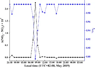
the one of NO + O3 reaction. Figure 4 presents the time evolution of hourly (NO2 − NOx) calculated from Eq.(2) and fNO2.
Overall, nitrogen oxide isotope effects appear to induce very small (NO2 − NOx) (see Fig. 4). They are found to be negligible
during the entire sampling period, except between 7:00 and 9:00 when hourly (NO2 − NOx) ranges from 0.5 to 2.3 ‰. This
largely reflects the fact that NOx is mostly under the form of NO2 (fNO2 = 1) except in the morning (see Fig. 2) due to direct
emissions of NO which decreases fNO2 (0.87 < fNO2 < 0.97 between 7:00 and 9:00; see Fig. 2). Our values are in good agreement
with the (NO2 − NOx) range (between 1.3 and 2.5 ‰) calculated from isotopic measurements at West Lafayette, USA (Walters
et al., 2018). Moreover, Li et al. (2020) calculated a mean (NO2 − NOx) of (1.3 ± 3.2) ‰ from isotopic measurements near
San Diego, USA (NOx concentration varied from 1 to 9 nmol mol−1). Overall, it appears that, in moderately polluted
275
environments, the small (NO2 − NOx) values are mostly due to high fNO2. In our case, the isotopic correction factor is only
significant for the sample collected between 6:00 and 9:00 to which we apply a 3 h mean correction factor of 1.0 ‰. This lowers δ15N(NO
2) from −4.9 to −5.9 ‰ but it still remains distinctively higher than for the other sampling time intervals.
Figure 4: Calculated isotopic fractionation values between NO2 and
NOx ((NO2 − NOx), solid black line) using Eq.(2) and fNO2 (dashed
blue line) during our sampling period.
Having accounting for isotope fractionation effects, we can assess the main possible NOx sources contribution at our site using
the US EPA source partitioning model IsoSource (EPA IsoSource Model, 2003) which solves numerically the following two-280 equation system: 15 N(NO2) = ∑ ( 𝑓𝑖× 15 N𝑖(NOx) 𝑖 ) (4) ∑ 𝑓𝑖 𝑖= 1 (5)
with 𝑓𝑖 the contribution proportion of source i and δ15Ni(NOx)the nitrogen isotopic composition of the NOx source i. We input
the isotopic signature of each sources influencing the nitrogen isotopic composition of NO2 and here we differentiate biogenic,
285
fuel combustion and traffic sources of NOx with distinctive δ15N means of −53.6, −17.9 and −2 ‰ respectively (Walters et al.,
2018). We set the source increment to 1 % and the mass balance tolerance of ± 5 %. As output, the model provides the most feasible source combinations and the descriptive statistics on the distribution for each source (Phillips and Gregg, 2003). According to the model results (see Fig. 5), traffic NOx emissions are dominant with a mean relative contribution of 0.82 ±
0.05 during the morning early hours against 0.62 ± 0.12 for the rest of the sampling period. Outside of traffic, fuel combustion 290
and biogenic sources account respectively for only 0.16 ± 0.08 and 0.03 ± 0.02 in the early morning against 0.29 ± 0.17 and 0.09 ± 0.05 for the rest of the sampling period. A very recent study (Barré et al., 2020) has estimated NO2 changes during the
COVID-19 lockdown combining satellite data (from the Tropospheric Monitoring Instrument), surface measurements and simulations (from the Copernicus Atmospheric Monitoring Service) and considering for weather variability that could bias the estimates. Interestingly, this study shows a NO2 reduction estimates around 50 % in Lyon, France during the lockdown period
295
in comparison of pre-lockdown concentration. If not strictly extrapolable to Grenoble because Lyon has a larger urban area (2 300 000 inhabitants), the NO2 column change in Lyon and the relative contribution of traffic in Grenoble NOx sources (68
%) inferred from N isotope values of NO2 are surprisingly close and comfort the idea that δ15N of NO2 is a very reliable tracer
of NOx emission sources after correction for LCIE and EIE.
Figure 5: NOx emission source partitioning using the
IsoSource EPA Model based on δ15N(NO
2) measured
during: the morning rush hours from 6:00 to 9:00 am local time (white boxes) and the other 3 h intervals (grey boxes). References values for each sources were taken from Walters et al. (2018).
4.2 Oxygen isotope composition
300
The time evolution of δ18O of atmospheric NO
2 (δ18O(NO2)) shown in Fig. 3 exhibits a substantial diurnal variation with a day
mean of (93.4 ± 13.9) ‰ and night mean of (68.9 ± 9.5) ‰. A maximum value of 114.5 ‰ is observed in the morning (09:00-12:00 interval) and a minimum value of 62.2 ‰ for the late-night interval (00:00-05:00). Using a similar sampling apparatus during summer in the urban/sub-urban site of West Lafayette, USA, Walters et al. (2018) reported δ18O(NO
2) daytime and
nighttime mean values of (86.5 ± 14.1) ‰ and (56.3 ± 7.1) ‰, respectively. Although our daytime values are higher than 305
those of Walters et al. (2018), both datasets exhibit the same day-night contrast with a maximum during the day and a minimum at night. As expected from δ18O values, Δ17O(NO
the 09:00-12:00 interval and a minimum value of 20.5 ‰ for the 00:00-05:00 interval. High Δ17O values are expected to reflect
the importance of ozone in the oxidation of NO to NO2. Since daytime and nighttime chemistries are radically different,
interpretation of our Δ17O measurements and their implications are discussed separately by day and night.
310
4.2.1 Fundamentals of NOx chemistry and isotopic transfers
NOx are mainly produced under the form of NO by combustion and lighting processes (Dennison et al., 2006; Young, 2002)
and by the biological activity of soils (Davidson and Kingerlee, 1997). In the daytime, NO and NO2 rapidly interconvert in a
time scale of about 1-2 minutes establishing a photostationary steady state (PSS; Leighton 1961): NO2 + h M → O(3P) + NO (R1) 315 O(3P) + O 2 M → O3 with M = N2 or O2 (R2) NO + O3 → NO2 + O2 (R3)
This so-called null cycle can be disturbed by RO2 radicals when NOx concentration are relatively high, typically above 30 pmol
mol−1 (Seinfeld and Pandis, 2006):
NO + RO2 → NO2 + RO (R4)
320
The reaction between NO and RO2 competes with the NO + O3 reaction, allowing NO2 formation without the consumption of
an ozone molecule in the cycle (Monks, 2005). This results in ozone production and can lead to severe ozone build up in polluted areas. At night, RO2 concentrations are strongly reduced making ozone the main NO oxidant following R3. NOx are
mainly removed from the atmosphere via the oxidation of NO2 into nitric acid during the day:
NO2 + OH → HNO3 (R5) 325 and at night : NO2 + O3 M → NO3 + O2 (R6) NO3 + NO2 M → N2O5 H2O, aerosol → 2 NHO3 (R7)
In this framework, Δ17O(NO
2) is driven by the relative importance of the different NO2 production channels because NO2 loss
processes do not fractionate in terms of oxygen mass-independent anomaly. Each NO2 production channel generates a specific
330
mass-independent isotopic anomaly Δ17O on the produced NO
2 (Kaiser et al., 2004). Based on the NO2 continuity equation,
this can be expressed with the following Δ17O(NO
2) mass-balance equation (Morin et al., 2011):
𝑑
𝑑𝑡([NO2] × 𝛥 17O(NO
with [NO2] being the atmospheric NO2 concentration, Pi and Lj the NO2 production/emission and loss rates (= concentration
of involved species multiplied by the kinetic constants of the considered chemical reaction), and Δ17O
i(NO2) the specific
335
isotope anomaly transferred to NO2 through the production reaction i.
4.2.2 Δ17O
day(NO2)
By day, the NOx photochemical cycle (R1 to R4) achieves a steady state in 1-2 minutes, which is several orders of magnitude
faster than NO2 loss reactions (Atkinson et al., 1997) and emission rate (NOx are mainly emitted under the form of NO; Villena
et al., 2011). It follows that NO and NO2 short variations can be neglected i.e.
𝑑
𝑑𝑡[NO2] 0 and 𝑑
𝑑𝑡[NO] 0 on short timescales. 340
In addition, fast interconversions between NO and NO2 generate quickly an isotopic equilibrium between NO and NO2
resulting in Δ17O(NO
2) Δ17O(NO) (Michalski et al., 2014; Morin et al., 2007). With these approximations, considering only
the main reactions and neglecting halogen chemistry, Eq.(6) yields to (Morin et al., 2007): 𝛥17O
day(NO2)
𝑘NO+O3[O3] × 𝛥17ONO+O3(NO2) + 𝑘NO+RO2[RO2] × 𝛥17ONO+RO2(NO2)
𝑘NO+O3[O3] + 𝑘NO+RO2[RO2] (7)
with Δ17O
NO+O3(NO2) being the ozone isotopic anomaly transferred to NO during its oxidation to NO2 via R3 (also called the
345
transfer function of the isotope anomaly of ozone to NO2; Savarino et al., 2008) and Δ17ONO+RO2(NO2) being the RO2 isotopic
anomaly transferred to NO during its oxidation to NO2 via R4. Δ17ONO+RO2(NO2) can be considered to be negligible (Alexander
et al., 2020; Michalski et al., 2003) because RO2 are mainly formed by the reactions R + O2 and H + O2 and the isotopic
anomaly of atmospheric O2 is very close to 0 ‰ (Barkan and Luz, 2003). This assumption has been estimated to affect the
overall Δ17O of RO
2 values by less than 1 ‰ (Röckmann et al., 2001). As a result, Eq.(7) can be simplified, giving a
350
Δ17O
day(NO2) driven by the relative importance of R3 (NO + O3) and R4 (NO + RO2) in the NO oxidation and by the oxygen
isotopic anomaly transferred from O3 to NO2:
𝛥17O
day(NO2) × 𝛥17ONO+O3(NO2) (8)
with = 𝑘NO+O3[O3]
𝑘NO+O3[O3] + 𝑘NO+RO2[RO2] (9)
Δ17O
NO+O3(NO2) has been determined experimentally by Savarino et al. (2008). They reported Δ17ONO+O3(NO2) = (1.18 ± 0.07
355
× Δ17O(O
3) + 6.6 ± 1.5) with Δ17O(O3) being the bulk ozone isotopic anomaly. Δ17O(O3) has been measured in Grenoble in
2012 (Vicars and Savarino, 2014); the mean measured Δ17O(O
3) was (26.2 ± 1.3) ‰ corresponding to a Δ17ONO+O3(NO2) value
of (37.5 ± 2.8) ‰ which, according to Eq.(8), would give a maximum Δ17O
day(NO2) value of (37.5 ± 2.8) ‰. It is consistent
with our maximum measured Δ17O(NO
2) value of 39.2 ‰ for the 09:00-12:00 interval. In light of the known uncertainties, the
small difference is not significant and is much smaller than the diurnal variations of Δ17O(NO
2). Note that the Δ17O calibration
360
is not very accurate for the most enriched samples because nitrite standards with high Δ17O are still not readily available. In a
laboratory study Michalski et al. (2014) measured the Δ17O of NO
reported Δ17O(NO
2) = (39.3 ± 1.9) ‰. Despite experimental conditions (e.g. NOx ≫ O3, light source, absence of VOCs) that
are not strictly applicable to our atmospheric conditions, their value is surprisingly close to our maximum value. Assuming that our maximum Δ17O(NO
2) value correspond to close to unity (R3 (NO + O3) ≫ R4 (NO + RO2)), we use a value of 39.2
365
‰ for Δ17O
NO+O3(NO2) for the following calculations. Combining Eq.(8) and Eq.(9), an expression for the RO2 concentration
can be derived as: [RO2] = 𝑘NO+O3× [O3] 𝑘NO+RO2 ( 𝛥17ONO+O3(NO2) 𝛥17O day(NO2) − 1) (10)
Figure 6 shows the estimated daytime evolution of and RO2. varies between 0.76 and 1 with a mean daytime of 0.86 (the
measured daytime Δ17O(NO
2) mean value is (33.5 ± 3.9) ‰) meaning that 86 % of NO2 is formed via R3 (oxidation of NO by
370
O3). The mean estimated RO2 concentration is (14.8 ± 12.5) pmol mol−1. Note that RO2 = 0 pmol mol−1 for the 09:00-12:00
interval originates from our assumption of = 1 for our highest Δ17O(NO
2) value; in reality, it only means that RO2 is so low
that R3 (NO + O3) ≫ R4 (NO + RO2). Overall, our RO2 values are found to be within the range of values measured at
urban/peri-urban sites (see Table 2). However, RO2 diurnal variation at our site do not follow the pattern of previous
measurements which usually report a diurnal variation with a maximum varying from noon to early afternoon (Fuchs et al., 375
2008; Tan et al., 2017) whereas this study shows a maximal concentration in late afternoon. Further investigations with additional more accurate measurements and the use of a chemical box-model is needed to interpret this RO2 behaviour.
380
385
390
Figure 6: (solid black slots) estimated from measured Δ17O of
atmospheric NO2 in Grenoble and RO2 concentrations (dashed
blue slots) derived from Eq.(10). Error bars for are derived from
standard deviation of Δ17O(NO
2) and Δ17O(O3*) measured in
Grenoble (Vicars and Savarino, 2014). RO2 error bars are derived
from O3 measurement uncertainties and errors on (by
comparison, errors on reaction constants can be neglected). The dashed vertical line indicates the local solar noon.
Site RO2 /pmol mol−1 Reference
Grenoble (2019, May) 0-35 (*) This study
UK, suburban site (2003, July-August) 4-22 Emmerson et al. (2007) Germany, suburban site (2005, July) 2-40 Fuchs et al. (2008) Germany, rural site (1998, July-August) 2-50 Mihelcic et al. (2003) USA, rural site (2002, May-June) 9-15 Ren et al. (2005) China, rural site (2014, June-July) 7-37 Tan et al. (2017) Table 2: Mean daytime RO2 concentration ranges measured during field campaigns in
various environments and seasons. (*) Derived from Eq.(6) using Δ17O values of atmospheric
NO2 in Grenoble.
Morin et al. (2011) simulated the diurnal variation of Δ17O(NO
2) in a remote marine boundary layer without the effect of
emissions. They assumed Δ17O(O
3) = 30 ‰ (Δ17ONO+O3(NO2) = 45‰) resulting into higher overall Δ17O(NO2) values compared
to our study. Their simulated Δ17O(NO
2) exhibited large diurnal variations with maximum values at night (close to 41 ‰) and
395
minimum values at noon of 28 ‰. This is consistent with RO2 concentration reaching a maximum around local noon in clean
environments. In contrast to their model simulations, our daytime Δ17O(NO
2) measurements are higher than our nighttime
measurements. We will show later that this difference originates from absence of NO emission in Morin et al., (2011) photochemical modelling.
4.2.3 Δ17O
night(NO2) 400
Without photolysis at night and associated RO2 production, ozone is the unique NO oxidant, and NO and NO2 are no longer
in photochemical equilibrium because NO2 cannot be converted back into NO. As a result, the oxygen isotopic composition
of NO2 formed during the night is determined by the oxygen isotopic composition of emitted NO and O3. Additionally, we
need to determine the residual fraction 𝑥(𝑡) of NO2 formed during the day that is still present at night in order to estimate the
overall isotopic signature of NO2 sampled at night following:
405 𝛥17O
night(NO2) 𝑥 × 𝛥17Oday(NO2) + (1 − 𝑥)
2 × (𝛥
17O
NO+O3(NO2) + 𝛥
17O(NO)) (11)
with 𝑥 being the residual fraction of NO2 formed during the day to the total NO2 measured at night and (1 – 𝑥) representing
the fraction of the total NO2 which has been produced during the night. NO is mainly emitted by combustion processes in
which a nitrogen atom (from atmospheric N2 or N present in fuel) is added to an oxygen atom formed by the thermal
decomposition of O2 (Zeldovich, 1946). With Δ17O(O2) being close to 0 ‰ (Barkan and Luz, 2003), NO is very likely to have
410
a Δ17O 0 ‰, or at least negligible compared to Δ17O
NO+O3(NO2). Using Eq.(11), along with a negligible isotope anomaly for
NO, the evolution of Δ17O(NO
2) over the night can be calculated. It is worth pointing out that the 𝑥 fraction becomes very
small at the end of the night allowing to simplify further Eq.(11) : 𝛥17O
night(NO2) 1 2× 𝛥
17O
NO+O3(NO2). Thus, if there are
nighttime NO emissions, a measurement of Δ17O(NO
2) at the end of the night is also an interesting way of deriving Δ17O(O3)
which is difficult to measure directly. The nighttime variation of the 𝑥 fraction is estimated considering that the nighttime 415
lifetime of NO2 relative to oxidation via ozone and dry deposition is 7.2 hours (O3 chemical sink is dominant over deposition
by a factor > 104 with 𝑘
NO2+O3 = 1.4×10⁻¹³ exp[−2470/T] cm3 molec−1 s−1 Atkinson et al., 2004; NO2 dry velocity Vd = 0.25 cm
s−1 Holland et al., 1999 and assuming a nighttime boundary layer height of 500 m). For the 00:00-05:00 interval, we calculate a mean value of Δ17O(NO
2) = 19.9‰ (with an overall error of about 1.6 ‰) which is very close to our measured Δ17O(NO2)
of 20.5 ‰. Overall, this first dataset of Δ17O(NO
2) nighttime measurements comes to confirm our understanding of nighttime
420
NO2 formation (Alexander et al., 2020; Michalski et al., 2014). NO emissions in urban areas have a very significant influence
on Δ17O(NO
2) leading to a behaviour in opposition to the one observed in remote locations. As illustrated by Morin et al.
(2011), Δ17O(NO
2) is predicted to be maximal at night in remote areas where NO emissions are negligible, reflecting the
isotopic signature of NO2 at sunset. In areas where nighttime NO emissions are high, nighttime Δ17O(NO2) can be up to a
factor of two smaller than in remote areas. 425
5 Conclusion
The primary goal of this preliminary work was to address an efficient and portable sampling system for atmospheric NO2
fitting with accurate isotopic analysis of double nitrogen and triple oxygen isotopes. First simultaneous measurements of the multi-isotopic composition (δ15N, δ18O, and Δ17O) of atmospheric NO
2 are reported here, notably at relatively high temporal
resolution (3 h). Over the course of more than one day in the Grenoble urban/suburban environment, δ15N values of NO 2 shows
430
little variation from −11.8 to −4.9 ‰ with negligible N isotopefractionations between NO and NO2 due to high NO2/NOx
ratios. NOx emissions main sources are estimated using a stable isotope model indicating a high probability of the
predominance of traffic NOx emissions in this area. We found Δ17O to vary diurnally with a maximum daytime value of (39.2
± 1.7) ‰ and a minimum night-time value of (20.5 ± 1.7) ‰. At photo-stationary state, high Δ17O(NO
2) values results from
the ozone predominance in NO oxidation pathways whereas lower values reflect the influence of peroxy radicals. We estimate 435
from Δ17O(NO
2) measurements that 86 % of NO2 produced by day originates from the oxidation of NO by O3. Moreover, a
mean daytime peroxy radical concentration of (14.8 ± 13.5) pmol mol−1 is derived from the oxygen isotopic measurements.At night, NOx photochemistry shutdowns and hence Δ17O(NO2) decreases under the growing influence of the isotopic footprint
from NO emitted by night. Our Δ17O(NO
2) measured during the middle/end of the night is quantitatively consistent with typical
values of Δ17O(O
3). The overall agreement between our measured values and laboratory studies argue for high accuracy of our
440
analytical field sampling method however nitrite standards with higher Δ17O value must be developed to further improve data
calibration. This work sheds light on the sensitivity of NO2 isotopic signature to the atmospheric chemical regimes and
emissions of the local environment. This isotopic approach can be applied to various environment in order to probe further the oxidative chemistry and help to constrain the NOx fate in a more quantitative way.
In the future, this method should be extended with a modelling tool such as a photochemical box model including isotopic 445
samplings and multi-isotopic analysis of atmospheric nitrate performed in parallel to those of NO2 would certainly be of interest
for the study of the full reactive nitrogen cycle.
Appendix A: Isotopic standards and calibration
This method of analysis induces isotope fractionations during NO2−/N2O conversion and ionization in the spectrometer, as well
450
as isotope exchanges between NO2− and its medium. Indeed, while isotope exchanges between nitrite and its matrix are
minimized due to the basic pH, the chemistry required to convert nitrite to N2O involves a step in an acidic medium that
promotes an exchange of oxygen isotopes (Casciotti et al., 2007). In order to eliminate the effects of these isotope splits, the system is calibrated using standards of known isotopic composition, which are subjected to the same treatment as the samples. This is called the identical treatment principle (Brand, 1996). By subjecting compounds of known isotopic composition to the 455
same treatment as the samples, the isotope fractionation induced by the manipulations can be estimated and the values of the samples can be corrected. Standards are first dissolved in a basic aqueous medium (pH = 12) and then, from this stock solution, five series of each standard are prepared in several concentration ranges, namely, 40 nmol, 80 nmol, 100 nmol, 120 nmol and 150 nmol in order to estimate the effects of the concentration of a material on its isotopic measurement. The matrix used for their preparation is the same as that of the samples, i.e. a mixture of KOH 2M/guaiacol in Milli-Q water. Correction factors 460
are obtained by linear regression between the raw and the expected values of δ15N, δ18O and δ17O of the standards. Three
international references of known δ15N and δ18O values are used for this work. These are nitrite salts, named RSIL-N7373,
RSIL-N10219 and RSIL-N23 with respective δ15N/δ18O values of –79.6/4.2 ‰, 2.8/88.5 ‰, and 3.7/11.4 ‰. Although the
three standards cover a wide range of isotopic composition in δ15N and δ18O, they do not have an isotopic anomaly in 17O. As
we are not aware of any available international reference nitrite standards with a known 17O anomaly, we are currently in the
465
process of manufacturing our own standards. As this step is still under development, and in order to be able to assess the accuracy of our 17O measurements of atmospheric NO
2 samples, we have estimated the isotope fractionation that 17O undergoes
during the analysis. RSIL-N7373 and RSIL-N23 standards having a Δ17O = 0 ‰ we estimate their 17O composition such that
δ17O = 0.52 × δ18O. For standard RSIL-N10219, we measure a negative Δ17O around −7 ‰. We therefore apply the mass
independent relation such that δ 17O
std(RSIL-N10219) = Δ17Oraw(RSIL-N10219) + 0.5 × δ18Ostd(RSIL-N10219).
470
The isotopic exchange of 18O is estimated at 11 % for standards at 100 nmol (Fig. A1) which is in line with Kobayashi et al.,
2020 who have estimated the degree of O isotope exchange in the azide method between H2O and NO2− to (10.8 ± 0.3) %. The 15N calibration curve allows us to ensure a good fractionation rate during the analysis. Indeed, given the 1:1 association of the
nitrogen atoms of nitrite and azide, the theoretical value of the calibration slope must be 0.5. The slight deviation from our measured value can be attributed to a blank effect, estimated here at 2 % of the size of the standards (6 % for those at 40 nmol). 475
480
485
Appendix B: Isotopic standards and calibration
Oxygen isotopes in nitrites are very labile (Böhlke et al., 2007) but the basic pH of the eluent limits isotopic exchanges. To ensure isotopic integrity from denuders extraction to analysis by IRMS, we followed Walters et al. (2018) procedure to quantify isotopic exchanges that might occur with the eluted matrix during storage. Thus, three solutions containing each 500 nmol of 490
KNO2 salts (RSIL-N7373, RSIL-N10219 and RSIL-N23) were prepared in the eluted matrix and kept frozen. 100 nmol were
collected from time to time from the individual solutions, analysed and refrozen until the next analysis. We monitored the nitrite standards isotopic composition prepared in the eluted guaiacol matrix during 22 days. The temporal evolution of the
δ17O, δ18O and Δ17O differences between our measurements of RSIL standards (prepared in the KOH/guaiacol eluted matrix)
and their certified reference values is plotted in Figure B1. It represents the temporal drift of the isotopic signal with respect 495
to reference values. If the deviation is constant, it means that the isotopic signal is not degraded with time and its standard deviation is considered as the uncertainty in our δ17O(NO
2) and δ18O(NO2) measurements. As shown in Fig. B1, deviations of
the three standards were stable over the 22-days experiment with an overall mean of (1.1 ± 0.8) ‰, (2.3 ± 1.8) ‰, and (−0.1 ± 0.3) ‰ for δ17O, δ18O and Δ17O respectively. Note that RSIL-N10219 shows higher δ17O and δ18O residuals than the two
other standards. The reason for this difference of behaviour is still not fully understood. As residuals remain steady over several 500
weeks, we consider this method suitable for the oxygen analysis of NO2 and the uncertainties applied to our isotopic
measurements are reported as the propagation error of the mean measurement uncertainty and the mean uncertainty resulting from NO2- storage. In our study, average uncertainties on δ17O, δ18O, and Δ17O are estimated to be ± 1.1, ± 2.5 and ±1.7 ‰,
respectively (1σ uncertainties). 505
Figure A1: Calibration of (a) 18O and (b) 15N with nitrite standards at 100 nmol measured by the chemical
azide method. The measured δ18O (δ18O
raw) and δ15N (δ15Nraw) values of NO2− standards are plotted against
their certified reference δ18O (δ18O
Figure B1: Temporal evolution of δ17O, δ18O and Δ17O differences between
our measurements of RSIL standards (prepared in the KOH/guaiacol eluted matrix) and their certified reference values. Error bars derived from measurement uncertainties are approximately equivalent to the size of the markers.
Author contribution. Sampling and analysis protocol were developed by SA under the supervision of JS. NC and AB
contributed with technical and knowledge support to SA for isotopic mass spectrometry and more general atmospheric 510
measurements. SB and JS, supervisors of SA PhD Thesis, helped SA in interpreting the results and writing the manuscript.
Competing interests. The authors have no conflict of interests to report.
Acknowlegements. The authors acknowledge the support of the ALPACA program (Alaskan Layered Pollution and Arctic
515
Chemical Analysis) funded by two French research organisms: the French polar institute (IPEV, Institut polaire français Paul-Emile Victor) and INSU-CNRS (National Institute of Sciences of the Universe) via its national LEFE program (Les Enveloppes Fluides et l'Environnement). This work benefited from the IGE infrastructures and laboratory platform PANDA which are partially supported by the ANR project ANR-15-IDEX-02 and Labex OSUG@2020, Investissements d’avenir – ANR10 LABX56. We would like to thank E. Gauthier, S. Darfeuil and P. Akers for help with laboratory work and more 520
References
Alexander, B., Hastings, M. G., Allman, D. J., Dachs, J., Thornton, J. A. and Kunasek, S. A.: Quantifying atmospheric nitrate formation pathways based on a global model of the oxygen isotopic composition (Δ17O) of atmospheric nitrate, Atmospheric
Chemistry and Physics, 9(14), 5043–5056, doi:https://doi.org/10.5194/acp-9-5043-2009, 2009. 525
Alexander, B., Sherwen, T., Holmes, C. D., Fisher, J. A., Chen, Q., Evans, M. J. and Kasibhatla, P.: Global inorganic nitrate production mechanisms: comparison of a global model with nitrate isotope observations, Atmospheric Chemistry and Physics, 20(6), 3859–3877, doi:https://doi.org/10.5194/acp-20-3859-2020, 2020.
Assonov, S. S. and Brenninkmeijer, C. a. M.: Reporting small Δ17O values: existing definitions and concepts, Rapid Communications in Mass Spectrometry, 19(5), 627–636, doi:https://doi.org/10.1002/rcm.1833, 2005.
530
Atkinson, R., Baulch, D. L., Cox, R. A., Hampson, R. F., Kerr, J. A., Rossi, M. J. and Troe, J.: Evaluated Kinetic, Photochemical and Heterogeneous Data for Atmospheric Chemistry: Supplement V. IUPAC Subcommittee on Gas Kinetic Data Evaluation for Atmospheric Chemistry, Journal of Physical and Chemical Reference Data, 26(3), 521–1011, doi:10.1063/1.556011, 1997.
Atkinson, R., Baulch, D. L., Cox, R. A., Crowley, J. N., Hampson, R. F., Hynes, R. G., Jenkin, M. E., Rossi, M. J. and Troe, 535
J.: Evaluated kinetic and photochemical data for atmospheric chemistry: Volume I - gas phase reactions of Ox, HOx, NOx and
SOx species, Atmospheric Chemistry and Physics, 4(6), 1461–1738, doi:https://doi.org/10.5194/acp-4-1461-2004, 2004.
Barkan, E. and Luz, B.: High-precision measurements of 17O/16O and 18O/16O of O
2 and O2/Ar ratio in air, Rapid Commun.
Mass Spectrom., 17(24), 2809–2814, doi:10.1002/rcm.1267, 2003.
Barré, J., Petetin, H., Colette, A., Guevara, M., Peuch, V.-H., Rouil, L., Engelen, R., Inness, A., Flemming, J., Pérez García-540
Pando, C., Bowdalo, D., Meleux, F., Geels, C., Christensen, J. H., Gauss, M., Benedictow, A., Tsyro, S., Friese, E., Struzewska, J., Kaminski, J. W., Douros, J., Timmermans, R., Robertson, L., Adani, M., Jorba, O., Joly, M. and Kouznetsov, R.: Estimating lockdown induced European NO2 changes, Atmospheric Chemistry and Physics Discussions, 1–28,
doi:https://doi.org/10.5194/acp-2020-995, 2020.
Böhlke, J. K., Smith, R. L. and Hannon, J. E.: Isotopic Analysis of N and O in Nitrite and Nitrate by Sequential Selective 545
Bacterial Reduction to N 2 O, Analytical Chemistry, 79(15), 5888–5895, doi:10.1021/ac070176k, 2007.
Brand, W. A.: High Precision Isotope Ratio Monitoring Techniques in Mass Spectrometry, Journal of Mass Spectrometry, 31(3), 225–235, doi:10.1002/(SICI)1096-9888(199603)31:3<225::AID-JMS319>3.0.CO;2-L, 1996.
Brown, S. S.: Variability in Nocturnal Nitrogen Oxide Processing and Its Role in Regional Air Quality, Science, 311(5757), 67–70, doi:10.1126/science.1120120, 2006.
550
Buttini, P., Di Palo, V. and Possanzini, M.: Coupling of denuder and ion chromatographic techniques for NO2 trace level
determination in air, Science of The Total Environment, 61, 59–72, doi:10.1016/0048-9697(87)90356-1, 1987.
Casciotti, K. L., Sigman, D. M., Hastings, M. G., Böhlke, J. K. and Hilkert, A.: Measurement of the oxygen isotopic composition of nitrate in seawater and freshwater using the denitrifier method, Analytical Chemistry, 74(19), 4905–4912, doi:10.1021/ac020113w, 2002.
555
Crutzen, P. J.: My life with O3, NOx and other YZOx compounds (Nobel lecture), Angewandte Chemie Int. Ed. Engl., 35, 1759
Dahal, B. and Hastings, M. G.: Technical considerations for the use of passive samplers to quantify the isotopic composition of NOx and NO2 using the denitrifier method, Atmospheric Environment, 143, 60–66, doi:10.1016/j.atmosenv.2016.08.006,
2016. 560
Davidson, E. A. and Kingerlee, W.: A global inventory of nitric oxide emissions from soils, Nutrient Cycling in Agroecosystems, 48(1), 37–50, doi:10.1023/A:1009738715891, 1997.
Dennison, P., Charoensiri, K., Roberts, D., Peterson, S. and Green, R.: Wildfire temperature and land cover modeling using hyperspectral data, Remote Sensing of Environment, 100(2), 212–222, doi:10.1016/j.rse.2005.10.007, 2006.
EPA IsoSource Model: Stable Isotope Mixing Models for Estimating Source Proportions, [online] Available from: 565
https://www.epa.gov/eco-research/stable-isotope-mixing-models-estimating-source-proportions (Accessed 15 October 2020), 2003.
Finlayson-Pitts, B. J. and Pitts, J. N.: Chemistry of the Upper and Lower Atmosphere, Elsevier., 2000.
Freyer, H. D., Kley, D., Volz‐Thomas, A. and Kobel, K.: On the interaction of isotopic exchange processes with photochemical reactions in atmospheric oxides of nitrogen, Journal of Geophysical Research: Atmospheres, 98(D8), 14791–14796, 570
doi:10.1029/93JD00874, 1993.
Fuchs, H., Holland, F. and Hofzumahaus, A.: Measurement of tropospheric RO2 and HO2 radicals by a laser-induced
fluorescence instrument, Review of Scientific Instruments, 79(8), 084104, doi:10.1063/1.2968712, 2008.
Galloway, J. N., Dentener, F. J., Capone, D. G., Boyer, E. W., Howarth, R. W., Seitzinger, S. P., Asner, G. P., Cleveland, C. C., Green, P. A., Holland, E. A., Karl, D. M., Michaels, A. F., Porter, J. H., Townsend, A. R. and Vöosmarty, C. J.: Nitrogen 575
Cycles: Past, Present, and Future, Biogeochemistry, 70(2), 153–226, doi:10.1007/s10533-004-0370-0, 2004.
Geng, F., Tie, X., Xu, J., Zhou, G., Peng, L., Gao, W., Tang, X. and Zhao, C.: Characterizations of ozone, NOx and VOCs
measured in Shanghai, China, Atmospheric Environment, 42(29), 6873–6883, doi:10.1016/j.atmosenv.2008.05.045, 2008. Harris, G. W., Carter, W. P. L., Winer, A. M., Pitts, J. N., Platt, Ulrich. and Perner, Dieter.: Observations of nitrous acid in the Los Angeles atmosphere and implications for predictions of ozone-precursor relationships, Environ. Sci. Technol., 16(7), 414– 580
419, doi:10.1021/es00101a009, 1982.
Holland, E. A., Dentener, F. J., Braswell, B. H. and Sulzman, J. M.: Contemporary and pre-industrial global reactive nitrogen budgets, Biogeochemistry, 46(1), 7–43, doi:10.1023/A:1006148011944, 1999.
Jacob, D. J.: Introduction to Atmospheric Chemistry, Princeton University Press [online] Available from: http://acmg.seas.harvard.edu/publications/jacobbook/bookchap11.pdf (Accessed 17 February 2020), 1999.
585
Jin, S. and Demerjian, K.: A photochemical box model for urban air quality study, Atmospheric Environment. Part B. Urban Atmosphere, 27(4), 371–387, doi:10.1016/0957-1272(93)90015-X, 1993.
Johnston, J. C. and Thiemens, M. H.: The isotopic composition of tropospheric ozone in three environments, J. Geophys. Res., 102(D21), 25395–25404, 1997.
Kaiser, J., Röckmann, T. and Brenninkmeijer, C. A. M.: Contribution of mass-dependent fractionation to the oxygen isotope 590
anomaly of atmospheric nitrous oxide, Journal of Geophysical Research: Atmospheres, 109(D3), D03305, doi:10.1029/2003JD004088, 2004.
Kaiser, J., Hastings, M. G., Houlton, B. Z., Röckmann, T. and Sigman, D. M.: Triple oxygen isotope analysis of nitrate using the denitrifier method and thermal decomposition of N2O, Anal. Chem., 79(2), 599–607, doi:10.1021/ac061022s, 2007.
Kaye, J. A.: Mechanisms and observations for isotope fractionation of molecular species in planetary atmospheres, Reviews 595
of Geophysics, 25(8), 1609–1658, doi:10.1029/RG025i008p01609, 1987.
Klein, A., Ravetta, F., Thomas, J. L., Ancellet, G., Augustin, P., Wilson, R., Dieudonné, E., Fourmentin, M., Delbarre, H. and Pelon, J.: Influence of vertical mixing and nighttime transport on surface ozone variability in the morning in Paris and the surrounding region, Atmospheric Environment, 197, 92–102, doi:10.1016/j.atmosenv.2018.10.009, 2019.
Kleinman, L. I., Daum, P. H., Lee, Y.-N., Nunnermacker, L. J., Springston, S. R., Weinstein‐Lloyd, J. and Rudolph, J.: Ozone 600
production efficiency in an urban area, Journal of Geophysical Research: Atmospheres, 107(D23), 4733, doi:10.1029/2002JD002529, 2002.
Kobayashi, K., Fukushima, K., Onishi, Y., Nishina, K., Makabe, A., Yano, M., Wankel, S. D., Koba, K. and Okabe, S.: Influence of δ18O of water on measurements of δ18O of nitrite and nitrate, Rapid Communications in Mass Spectrometry, n/a(n/a), doi:10.1002/rcm.8979, 2020.
605
Krankowsky, D., Bartecki, F., Klees, G. G., Mauersberger, K., Schellenbach, K. and Stehr, J.: Measurement of heavy isotope enrichment in tropospheric ozone, Geophys. Res. Lett., 22(13), 1713–1716, 1995.
Largeron, Y. and Staquet, C.: Persistent inversion dynamics and wintertime PM10 air pollution in Alpine valleys, Atmospheric Environment, 135, 92–108, doi:10.1016/j.atmosenv.2016.03.045, 2016.
Leighton, P. A.: Photochemistry of Air Pollution., Academic Press, 66(3), 279–279, doi:10.1002/bbpc.19620660323, 1961. 610
Li, J., Zhang, X., Orlando, J., Tyndall, G. and Michalski, G.: Quantifying the nitrogen isotope effects during photochemical equilibrium between NO and NO2: implications for δ15N in tropospheric reactive nitrogen, Atmospheric Chemistry and
Physics, 20(16), 9805–9819, doi:https://doi.org/10.5194/acp-20-9805-2020, 2020.
Li, W., Ni, B. L., Jin, D. Q. and Zhang, Q. G.: Measurement of the absolute abundance of Oxygen -17 in SMOW, Kexue Tongboa, Chinese Science Bulletin, 33 (19), 1610–1613, doi:10.1360/sb1988-33-19-1610, 1988.
615
Liao, H. and Seinfeld, J. H.: Global impacts of gas-phase chemistry-aerosol interactions on direct radiative forcing by anthropogenic aerosols and ozone, Journal of Geophysical Research: Atmospheres, 110(D18), doi:10.1029/2005JD005907, 2005.
Lyons, J. R.: Transfer of mass-independent fractionation in ozone to other oxygen-containing radicals in the atmosphere, Geophysical Research Letters, 28(17), 3231–3234, doi:10.1029/2000GL012791, 2001.
620
Mariotti, A.: Natural 15 N abundance measurements and atmospheric nitrogen standard calibration, Nature, 311(5983), 251, doi:10.1038/311251a0, 1984.
Mayer, H.: Air pollution in cities, Atmospheric Environment, 33(24), 4029–4037, doi:10.1016/S1352-2310(99)00144-2, 1999. McIlvin, M. R. and Altabet, M. A.: Chemical Conversion of Nitrate and Nitrite to Nitrous Oxide for Nitrogen and Oxygen Isotopic Analysis in Freshwater and Seawater, Analytical Chemistry, 77(17), 5589–5595, doi:10.1021/ac050528s, 2005. 625
Michalski, G., Scott, Z., Kabiling, M. and Thiemens, M. H.: First measurements and modeling of Δ17O in atmospheric nitrate.,