HAL Id: hal-00411913
https://hal.archives-ouvertes.fr/hal-00411913
Submitted on 31 Aug 2009
HAL is a multi-disciplinary open access
archive for the deposit and dissemination of
sci-entific research documents, whether they are
pub-lished or not. The documents may come from
teaching and research institutions in France or
abroad, or from public or private research centers.
L’archive ouverte pluridisciplinaire HAL, est
destinée au dépôt et à la diffusion de documents
scientifiques de niveau recherche, publiés ou non,
émanant des établissements d’enseignement et de
recherche français ou étrangers, des laboratoires
publics ou privés.
Large mass self-similar solutions of the
parabolic-parabolic Keller–Segel model of chemotaxis
Piotr Biler, Lucilla Corrias, Jean Dolbeault
To cite this version:
Piotr Biler, Lucilla Corrias, Jean Dolbeault.
Large mass self-similar solutions of the
parabolic-parabolic Keller–Segel model of chemotaxis. Journal of Mathematical Biology, Springer Verlag
(Ger-many), 2011, 63, pp.1-32. �10.1007/s00285-010-0357-5�. �hal-00411913�
Keller–Segel model of chemotaxis
Piotr Biler · Lucilla Corrias · Jean DolbeaultAugust 31, 2009
Abstract In two space dimensions, the parabolic-parabolic Keller–Segel system shares many properties with the parabolic-elliptic Keller–Segel system. In particular, solutions globally exist in both cases as long as their mass is less than 8 π. However, this threshold is not as clear in the parabolic-parabolic case as it is in the parabolic-elliptic case, in which solutions with mass above 8 π always blow up. Here we study forward self-similar solutions of the parabolic-parabolic Keller–Segel system and prove that, in some cases, such solutions globally exist even if their total mass is above 8 π, which is forbidden in the parabolic-elliptic case.
Keywords Keller–Segel model · chemotaxis · self-similar solution · nonlocal parabolic equations · critical mass · existence · blowup
Mathematics Subject Classification (2000) 35B30 · 35K40 · 35K57 · 35J60
1 Introduction
The Keller–Segel model has been widely studied for almost forty years. It models the behavior of a slime mold of myxamoebae, Dictyostelium Discoideum, which have the peculiarity of organizing themselves to form aggregates by moving towards regions of a higher concentration of a chemoattractant. This chemoattractant, the cyclic
adeno-sine monophosphate, is secreted by the amoebae themselves when they are lacking
of nutrients. The Keller–Segel model is considered as a prototypical model for pat-tern formation in chemotaxis, and has attracted a lot of attention as a test case for
P. Biler
Instytut Matematyczny, Uniwersytet Wroc lawski, pl. Grunwaldzki 2/4, 50–384 Wroc law, Poland. E-mail: Piotr.Biler@math.uni.wroc.pl
L. Corrias
D´epartement de Math´ematiques, Universit´e d’ ´Evry Val d’Essonne, rue du p`ere Jarlan, F-91025 ´
Evry C´edex, France. E-mail: lucilla.corrias@univ-evry.fr J. Dolbeault
Ceremade (UMR CNRS 7534), Universit´e Paris-Dauphine, Place de Lattre de Tassigny, F-75775 Paris C´edex 16, France. E-mail: dolbeaul@ceremade.dauphine.fr
more complex taxis phenomena driven by chemical substances. See [9, 10, 11, 17, 18] for further references.
The simplest version of the model is made of two equations, one for the density of the amoebae and another one for the density of the chemoattractant. Both are parabolic, although an even simpler version has been widely considered by neglecting the time-dependence of the density of the chemoattractant. We shall refer to the com-plete version of the model as the parabolic-parabolic model, and to the latter as the parabolic-elliptic Keller–Segel model.
The precise dependence of the diffusion coefficients and of the chemosensitivity parameter depends on the context. All variants of the model involve diffusions in the equations for the density of the amoebae and for the density of the chemoattractant. The coupling is due to the fact that amoebae move according to the gradient of the chemoattractant, and that the emission of the chemoattractant is proportional to the density of amoebae. A crude insight into the main features of the model can be gained from the simplest case, that is when the nonlinear term in the equation is quadratic, but more realistic models should probably involve more complex nonlinearities.
Since the slime mold usually moves over a planar substrate, it makes sense to consider two-dimensional geometries. In some cases, boundary effects are important, but they are out of the purpose of this paper and we shall therefore assume that the model is set on the two-dimensional Euclidean plane.
In the parabolic-elliptic model, there is a critical mass, 8 π after a proper adimen-sionalization, whose role is now rather well understood; see [8, 5]. Below such a mass, the diffusion predominates, in the sense that amoebae are unable to emit enough chemoat-tractant to aggregate. On large times, the population diffuses and locally vanishes, although the behavior significantly differs from a pure diffusion. Above 8 π, at least one singularity appears in finite time, which is interpreted as the occurrence of an aggregate.
Since singularities are local, it is widely believed that 8 π should also be a threshold between the diffusion dominated regime and the regime of aggregation also in the parabolic-parabolic model. This is certainly the case in some sense, for appropriate initial data, but the situation is not as simple as in the parabolic-elliptic case. It turns out that if, initially, the population of amoebae is scattered enough, and for a well chosen initial distribution of the chemoattractant, there are solutions for which the diffusion predominates for large times, even for masses larger than 8 π. It is the purpose of this paper to establish such a fact, for a special class of solutions and in a certain range of the parameters of the model.
In this paper, we consider the parabolic-parabolic Keller–Segel model
nt= ∆n − ∇ · (n ∇c) , (1)
τ ct= ∆c + n , (2)
for the densities n and c of, respectively, microorganisms (e.g. amoebae) and diffusing chemicals that they are secreting. Interesting mathematical questions are related to qualitative properties of problem (1)–(2) such as global in time existence versus finite time blowup of solutions describing chemotactic concentration phenomena. After the pioneering works of Keller and Segel, a huge literature has dealt with the mathematical modelling of chemotaxis and its analysis. We recommend the reading of [9] for a recent review from both biological and mathematical points of view.
We shall consider the Keller–Segel system (1)–(2) for any t > 0, x ∈ R2, supple-mented with initial conditions n0and c0. From now on we shall assume that n0and c0
are nonnegative and that n0 is integrable on R2. As a consequence, for solutions with
sufficiently fast decay at infinity, the total mass is conserved, i.e., M := Z R2 n(t, x) dx = Z R2 n0(x) dx
does not depend on t.
Throughout the paper, τ is a nonnegative parameter taking into account the differ-ence of the time scales of the diffusive processes undergone by n and c. The qualitative properties of n and c (such as the asymptotic behavior for large values of t) depend on τ and the stability of system (1)–(2) with respect to τ is expected, i.e. solutions of the parabolic-parabolic Keller–Segel system are expected to converge to those of parabolic-elliptic system when τ ց 0. This has been recently proved, at least for solu-tions with a suitably small mass M , in [16]. Here, we are interested in the differences between the parabolic-elliptic Keller–Segel system (τ = 0) and the parabolic-parabolic Keller–Segel system (τ > 0). Known results are briefly summarized as follows.
When τ = 0 in (2), M = 8 π is a threshold for existence versus blowup of the solution of (1)–(2), see [8, 5, 7]. Solutions globally exist for M < 8 π, while explosion in finite time may occur if M > 8 π. In the critical case M = 8 π, the solutions are known to be global in time but the density grows and mass concentration occurs in infinite time; see [3, 4].
For τ > 0, according to [7], solutions globally exist for any M < 8 π. However, it has not yet been proved that explosion occurs in finite time as soon as M > 8 π, for instance under some additional assumptions like a smallness condition onRR2|x|
2n
0(x) dx. If
M = 8 π, there is an infinite number of steady states (see [3]), but no other result is available, apart from self-similar solutions.
Motivated by this lack of results for (1)–(2), this paper deals with the existence of
positive forward self-similar solutions of (1)–(2), i.e., solutions which can be written as
n(t, x) =1 tu „ x √ t « and c(t, x) = v „ x √ t « , (3)
with a large total mass (that is, larger than 8 π). Indeed, since we are dealing with the two-dimensional case, any self-similar solution n in L1(R2) preserves mass, i.e., for
each t ≥ 0 Z R2 n(t, x) dx = Z R2 u(ξ) dξ = M .
Therefore, for any given τ > 0, we are interested in the optimal range of M for the existence of such solutions, and in uniqueness or multiplicity issues for a given M in the optimal range. Actually, our goal is double. The main one is to prove the above mentioned existence result. Second, we will give an as complete as possible review of the numerous existing results on the topic and also simplified, new proofs of them. For this reason, the remainder of the introduction will be primarily devoted to the state of the art on self-similar solutions.
Self-similar solutions can be obtained through various approaches. The first method for the study of self-similar solutions (see for example [1] and the references therein)
amounts to look for mild solutions of (1)–(2), that is, solutions of n(t, ·) = e(t−t0)∆n(t 0, ·) − Zt t0 “ ∇e(t−s)∆”·`n(s, ·) ∇c(s, ·)´ds , c(t, ·) = et−t0τ ∆c(t 0, ·) +1 τ Z t t0 et−sτ ∆n(s, ·) ds ,
for any t > t0≥ 0. Roughly speaking, such self-similar solutions are obtained by a fixed
point theorem. However, smallness conditions on the initial data are required in order to apply a contraction mapping principle; see [14], where this method has been applied to (1)–(2) with τ = 1. Therefore, covering the whole range of masses for which solutions exists seems out of reach in this setting.
Alternatively, one can prove the existence of self-similar solutions through the direct analysis of the elliptic system satisfied by (u, v), i.e.,
∆u − ∇ · „ u ∇v −12ξ u « = 0 , (4) ∆v +τ 2ξ · ∇v + u = 0 , (5)
where ξ = x/√t and the differential operators in (4)–(5) are taken with respect to ξ. In this case, a natural functional space to be considered for both u and v is the subspace C02(R2) of functions in the space C2(R2) such that
lim
|ξ|→∞u(ξ) = 0 and |ξ|→∞lim v(ξ) = 0 .
For such classical solutions, equation (4) can be written equivalently as either ∇ · » u ∇ „ log u − v +|ξ| 2 4 «– = 0 , or ∇ ·heve−|ξ|2/4∇“u e−ve|ξ|2/4”i= 0 .
Then, using the fact that u, v, and consequently |∇v| are bounded, it has been proved in [15] that there exists a constant σ such that
u(ξ) = σ ev(ξ)e−|ξ|24 (6)
for any ξ ∈ R2. Since u is positive by the maximum principle, it follows that σ is positive. As a consequence, u ∈ L1(R2), and the stationary system (4)–(5) reduces to a family of nonlinear elliptic equations for v, namely
∆v +τ
2ξ · ∇v + σ e
ve−|ξ|24 = 0 , (7)
parametrized by σ > 0. Again by the maximum principle applied to (7), the following upper bound for v can be proved
v(ξ) ≤ C e− min{1,τ }|ξ|24 , (8)
where C is any positive constant such that C min{1, τ } ≥ σ ekvk∞; see for instance [15]. Therefore, v ∈ L1(R2) holds true for any solution of (7) in C02(R2).
The range of M for which self-similar solutions exist in C02(R2) gives an indication on the range of M for which some solutions of (1)–(2) may globally exist. Self-similar solutions indeed provide explicit examples of global solutions, even with smooth initial data, up to a time-shift: take for instance u and v as the initial data for (1)–(2). Moreover, if self-similar solutions describe the asymptotic behavior of any solution of (1)–(2) under appropriate conditions on initial data, then the ranges of global existence of solutions should be exactly the same. This property has been established in [5] for τ = 0. In the case τ > 0, this might not be as simple as in the case τ = 0 if one can prove that blowup may occur for any M > 8 π. However, at least for initial data close enough to u and v, one can expect that the ranges of global existence are the same.
In view of our main goal, we are actually more interested in parametrizing the set of C02(R2) self-similar solutions in terms of mass rather than in terms of σ. This is possible using in (7) the relation
M = σ Z
R2
ev(ξ)e−|ξ|24 dξ . (9)
However, by doing that, equation (7) becomes nonlocal, as was the original system (1)–(2), and the problem is definitely more difficult to handle. Another not less im-portant reason to consider a different but equivalent formulation of problem (4)–(5) is that the correspondence between σ and M is not clear due to the lack of uniqueness of solutions to (7); see Remark 1 at the end of Section 2.
For the sake of completeness, we have to say that equation (7), written as ∇ ·“eτ4|ξ|
2
∇v”+ σ eveτ −14 |ξ| 2
= 0 ,
has been studied using variational methods in [13, 19]. The weighted functional space H1(R2; exp(τ4|ξ|2) dξ) is then natural, but working in this space introduces a condition on the values of τ , which have to be in the interval (0, 2). Under such a restriction, it has been established that solutions exist if 0 < σ < σ∗, for some σ∗ > 0. These solutions are positive and belong to C02(R2), but due to the restriction on τ , one has to look for alternative approaches.
Another important and useful result has been obtained in [15] using the moving planes technique: any positive solution v ∈ C02(R2) of (7) must be radially symmetric.
As a consequence, system (4)–(5) reduces to the ODE system u′− u v′+1 2r u = 0 , (10) v′′+ „1 r+ τ 2r « v′+ u = 0 , (11)
where u and v are considered as functions of the radial variable r = |ξ| only. Equations (6)–(7) then become u(r) = σ ev(r)e−r2/4, v′′+ „1 r+ τ 2r « v′+ σ eve−r2/4= 0 . (12)
Equation (12) has been studied in [12, 15]. More specifically, the authors proved in [12] the existence of a positive decreasing solution of (12) endowed with the initial
and integrability conditions
v′(0) = 0 and Z ∞
0 r v(r) dr < ∞ ,
(13) for any τ > 0 and σ > 0 such that σlog ττ −1 < 1/e (see Remark 2). However, such a condition does not determine the optimal range neither for the parameter σ nor for M .
It is worth noticing that the boundary conditions (13) and the following ones, v′(0) = 0 and lim
r→∞v(r) = 0 , (14)
are equivalent for classical decreasing solutions. Indeed, (13) implies (14) and the con-verse holds true by (8). Using (14), equation (12) turns out to be equivalent to
w′′+ „ 1 r+ τ 2r « w′+ ewe−r2/4= 0 , (15) w′(0) = 0 and w(0) = s , (16)
for some shooting parameter s ∈ R. Indeed, if w(r; s) is a classical solution of (15)– (16) for a given s ∈ R, then w(∞; s) = limr→∞w(r; s) exists and is finite and v(r) =
w(r; s) − w(∞; s) is a classical solution of (12)–(14) with σ = ew(∞;s). Conversely, if v is a classical solution of (12)–(14), then w(r; s) = v(r) + log σ is a classical solution of (15)–(16) with s = v(0) + log σ and again σ = ew(∞;s) holds true. It follows that all solutions of (12)–(14) can be parametrized in terms of s. See [15] for more details. Using this equivalence, the authors of [15] analyze the structure of the set of solutions of (12)–(14) seen as a one-parameter family; see Remark 1 at the end of Section 2. Computations presented in Figs. 1 have been based on this parametrization of the solution set.
Last but not least, the parametrization of the solutions of (15)–(16) in terms of s allows us to parametrize the total mass M in term of s by
M (s) = 2 π Z ∞
0
ew(r;s)e−r2/4r dr . (17) But again, this does not provide an explicit computation for the optimal range of M . Computations presented in Fig. 2 (left) have also been based on this parametrization of M .
Being this the state of the art, we will establish that the formulation of system (10)–(11) in terms of cumulated densities is better adapted to the qualitative descrip-tion of u and v. This is a classical technique used previously, for example, in the context of the parabolic-elliptic Keller–Segel system and astrophysical models; see [1, 3] and fur-ther references fur-therein. For τ > 0, many qualitative properties of the solutions can still be proved in this framework. These will allow us to build positive forward self-similar
solutions of (1)–(2) satisfying (3), which have an arbitrarily large mass when τ is large
enough. The obtained results are summarized in the theorem below. One may inter-pret it by saying that the diffusion of c described by (2) for positive large τ and some M > 8 π may prevent the blowup of the solutions of the parabolic-parabolic Keller– Segel system. This is a major difference with the parabolic-elliptic case τ = 0, for which the response of c to the variations of n being instantaneous, any smooth solution with mass M > 8 π must concentrate and blow up in finite time.
Theorem 1 For any M > 0, there exists some ˜τ (M ) ≥ 0 such that for any τ ≥ ˜τ(M)
there is at least one solution (u, v) of (4)–(5) in (C02(R2))2 with u > 0 of mass M and v > 0. If M < 8 π, ˜τ (M ) = 0. If M > 8 π, ˜τ (M ) is positive and there are
at least two solutions, except for the maximal possible value of M . All solutions are radial, nonincreasing, with fast decay at infinity, and hence attain their maximum at
x = 0. They are uniquely determined by a := u(0)/2, which in turn uniquely determines M = M (a, τ ). Moreover, lima→∞M (a, τ ) = 8 π, while, as a → ∞, the corresponding
solution u concentrates into a Dirac delta distribution, up to the factor 8 π, and v(0) =
kvkL∞(R2) becomes arbitrarily large.
This paper is organized as follows. We shall first establish the main a priori es-timates for Theorem 1 in the next section. The framework of cumulated densities is developed in Section 3, which also contains more detailed statements than the ones of Theorem 1. The remaining a priori estimates and proofs are given in Sections 4 and 5, respectively. Section 6 is devoted to some numerical results and Section 7 to concluding remarks.
2 Large mass positive forward self-similar solutions
Before restating the question of self-similar solutions in terms of cumulated densities, let us establish the key a priori estimate for Theorem 1, which proves that these solutions may have an arbitrary large mass when τ is large enough. This result is entirely new. Such an estimate can be obtained both from equation (12) and from the cumulated densities formulation. In this section, we shall establish this a priori estimate in the first setting. It will be translated in the cumulated densities framework in Section 4.
From now on, we shall parametrize M in term of a and τ , i.e. M = M (a, τ ), where a = u(0)/2 will be the shooting parameter in the cumulated densities shooting problem, see (29)–(30) and (33)–(34) below.
A positive classical solution v of (12), (14) solves “
r eτ r2/4v′”′+ σ r e(τ −1) r2/4ev= 0 , which, after an integration on (0, r), gives
v′(r) = −σr e−τ r2/4 Zr
0
e(τ −1) z2/4ev(z)z dz . (18) As a consequence, v′ is nonpositive, so that v(z) ≤ v(0) for any z ≥ 0 and, for τ 6= 1,
v′(r) ≥ −σr e−τ r2/4ev(0) Zr 0 e(τ −1) z2/4z dz = − 2 τ − 1 σ r e v(0)“e−r2/4 − e−τ r2/4”. (19) We observe that d dτ Z ∞ 0 “ e−r2/4− e−τ r2/4” 2 drr = Z ∞ 0 e−τ r2/4r 2dr = 1 τ . Hence, after one more integration of (19) on (0, ∞), we get, for any τ 6= 1,
v(0) ≤ σ ev(0)I(τ ) with I(τ ) := log τ
Actually, it is easy to check that estimate (20) holds true also for τ = 1 with I(1) = 1. Since from (6) we have
σ ev(0)= u(0) = 2 a , (21)
it has been proved that for each τ > 0, 0 = lim
z→∞v(z) ≤ v(r) ≤ v(0) ≤ 2 a I(τ ) (22)
for any r ∈ R+. On the other hand, by (9), (14) and (22), mass can be estimated for
any positive a and τ by M = 2 π σ Z ∞ 0 ev(r)e−r2/4r dr ≥ 2 π σ Z ∞ 0 e−r2/4r dr = 4 π σ ≥ 8 π a e−2 a I(τ ) (23) using (21). As a function of a, fM (a, τ ) := 8 π a e−2 a I(τ ) achieves its maximum at a∗(τ ) := 2 I(τ )1 , which proves that M = M (a, τ ) verifies for each τ > 0
max
a>0M (a, τ ) ≥ fM (a∗(τ ), τ ) =
4 π e I(τ ),
and it is clear that the right hand side can be made arbitrarily large for τ large enough. Hence, the corresponding density u(r) = σ ev(r)e−r2/4 has mass M > 8 π if e I(τ )4 π > 8 π, that is for any τ > ¯τ with ¯τ such that I(¯τ ) = 2 e1 , i.e. ¯τ ≈ 16.1109. Also observe that for any τ > ¯τ the density u corresponding to a = a∗(τ ) satisfies u(0) = 2 a∗(τ ) > 2 e. Finally, using v(z) ≥ v(r) in (18) and integrating the inequality on (0, ∞), one obtains e−v(0)− limr→∞e−v(r) ≤ − σ I(τ ), for any τ > 0. As a consequence, using (21) and
limr→∞e−v(r)= 1, we obtain that
1 − ev(0)≤ − σ I(τ ) ev(0)= − 2 a I(τ ) . This gives the estimate
v(0) > log(2 a I(τ ) + 1) , (24)
which implies that v(0) becomes arbitrarily large as a → ∞, for any τ > 0.
Estimates (23) and (24) can be read also as lower and upper bounds for σ = 2 a e−v(0), namely 2 a e−2 a I(τ )≤ σ ≤ min M 4 π, 2 a 2 a I(τ ) + 1 ff , (25)
hence showing that σ takes arbitrarily large values for τ large enough.
Remark 1 Estimates (25) on σ are new. The authors of [15] analyzed the map s 7→
σ(s), where s is the shooting parameter defined in (16), and they proved that it is a continuous map from R into R+ with lims→±∞σ(s) = 0. Therefore, σ must be
bounded for any fixed τ by σ∗ = σ(s∗), for some s∗ ∈ R, and problem (12)–(14) admits no solution for σ > σ∗, at least one solution for σ = σ∗ and finally (at least) two distinct solutions for 0 < σ < σ∗. However, estimates on σ (or σ∗) were missing.
Remark 2 Estimate (20) says that, for any fixed σ > 0 and τ > 0, v(0) satisfies
v(0) − σ I(τ ) ev(0)≤ 0 .
Since the function x 7→ x − σ I(τ ) ex is strictly concave and attains the maximum in x = − log(σ I(τ )), we deduce that whenever σ I(τ ) < 1/e, there exists an open interval J ⊂ R+ of non existence of solutions of (12) satisfying (14), with v(0) ∈ J. On the
3 Cumulated densities and main results
Let us introduce the cumulated densities formulation of the parabolic-parabolic Keller– Segel model as in [1], in terms of the functions u and v which solve problem (10)–(11), by defining φ(y) := 1 2 π Z B(0,√y) u(ξ) dξ = Z √y 0 r u(r) dr , ψ(y) := 1 2 π Z B(0,√y) v(ξ) dξ = Z √y 0 r v(r) dr . Using the relations
φ′(y) =1 2u ( √y) and φ′′(y) = 1 4 √yu ′(√y) , (26) ψ′(y) =1 2v ( √y) and ψ′′(y) = 1 4 √yv ′(√y) ,
it follows from (10)–(11) that the cumulated densities φ and ψ solve the second order ODE system
φ′′+1 4φ
′− 2 φ′ψ′′= 0 , (27)
4 y ψ′′+ τ y ψ′− τ ψ + φ = 0 , (28)
where (11) has been multiplied by r and integrated on (0, √y). Observing that equa-tion (28) can be written as
4 (y ψ′− ψ)′+ τ (y ψ′− ψ) + φ = 0 ,
and defining S(y) := 4 (ψ(y) − y ψ′(y))′ = −4 y ψ′′(y) = −√y v′(√y) as in [2, 15], system (27)–(28) becomes, after a differentiation of (28) with respect to y, a first order system in the (φ′, S) variables
φ′′+1 4φ ′+ 1 2 yφ ′S = 0 , (29) S′+τ 4S = φ ′. (30)
The last formulation of the ODE system can be equivalently written as a single integro-differential equation, hence nonlocal, for φ′,
φ′′+1 4φ ′+ 1 2 yφ ′e−τ y/4Z y 0 eτ z/4φ′(z) dz = 0 , (31) since, by (30), S(y) = e−τ y/4 Zy 0 eτ z/4φ′(z) dz , (32) and as a single, local but nonlinear second order ODE for S,
S′′+1 4(τ + 1) S ′+ τ 16S + 1 2 y “ S S′+τ 4S 2” = 0 ,
which is obtained by differentiating (30). We will use in the sequel all these formulations in order to get a priori estimates.
For any positive self-similar solution (u, v) ∈ (C02(R2))2, the natural initial
condi-tions for (29)–(30) are
φ(0) = 0 , φ′(0) = a > 0 and S(0) = 0 , (33) in view of the definition of φ and of (32). Moreover, for any self-similar solution u ∈ L1(R2), the corresponding cumulated density φ satisfies the boundary condition
φ(∞) := lim
y→∞φ(y) =
M (a, τ )
2 π . (34)
The problem is now formulated in terms of a shooting parameter problem (29)–(30), (33), with a new shooting parameter a which is directly related to the concentration of the self-similar density u around the origin, since a = u(0)/2. This has been obtained in Section 2 and will be made more precise below. Let us observe that the relation between a and the shooting parameter s defined in (16) is 2 a = es, since s = v(0) + log σ. Thus, a one-to-one relation is established between the initial valued problems (29)–(30), (33) and (15)–(16) as soon as an existence and uniqueness result is established for one of them. Moreover, we have
v(0) = v(√y) + 1 2 Zy 0 S(z) z dz , and the boundary condition limr→∞v(r) = 0 is equivalent to
v(0) = 1 2 Z ∞ 0 S(z) z dz . (35)
We also have: σ = limr→∞u(r) er
2/4
= 2 limy→∞φ′(y) ey/4. Hence we can
reparame-trize v(0) and σ in terms of a and τ .
The main statements we are going to prove are summarized in the following theo-rems. The a priori estimates will be established in Section 4. The proofs will be given in Section 5. We shall say that (φ, S) is a positive solution if both φ and S are positive functions.
Theorem 2 For any (a, τ ) ∈ R2+there exists a unique positive solution (φ, S) of (29)–
(30), (33) such that φ ∈ C2(0, ∞) ∩ C1[0, ∞) and S ∈ C1[0, ∞). Moreover, for any
fixed τ > 0, φ ∈ C2[0, ∞), the maps a ∈ R+7→ (φ, S) and a ∈ R+ 7→ M(a, τ ) ∈ R+
are continuous and
g(a, τ ) ≤M (a, τ )2 π ≤ f(a, τ ) ,
where f (a, τ ) = 8 > > > > > > < > > > > > > : min{4, 4 a} if τ ∈`0,12˜, minn4 a,23π2o if τ ∈`12, 1 ˜ , minn4 a,23π2τ, 4 (τ + 1)o if τ > 1 , (36)
and g(a, τ ) = 8 > > < > > : maxn4 a e−2 alogτ −1τ,4 a τ a+τ o if τ ∈ (0, 1] , maxn4 a e−2 alogτ −1τ, 4 a a+1 o if τ > 1 . (37)
For consistency, it is worth noticing that the inequality g(a, τ ) ≤ f(a, τ ) holds for all τ > 0 and a > 0.
Theorem 3 Given any fixed τ > 0, for any positive sequence {ak} such that ak→ ∞
as k → ∞, there exists a sequence of positive self-similar solutions (uk, vk) ∈ (C02(R2))2
satisfying (4)–(5) and uk(0) = 2 ak, v′k(0) = 0 such that
uk⇀ 8 π δ0 as k → ∞
in the sense of weak convergence of measures. Moreover, limk→∞RR2ukdx = 8 π and
limk→∞kvkkL∞(R2) = ∞.
Theorem 3 has already been proved in [15, Th. 2, (iii)] using a classical result by Brezis and Merle in [6]. However, here we shall give a simplified and quite direct proof using the cumulated densities formulation.
Theorem 4 For any fixed τ > 0 there exists M∗ = M∗(τ ) ≥ 8 π such that problem (29)–(30) with the boundary conditions
φ(0) = 0 , lim
y→∞φ(y) =
M
2 π, S(0) = 0 ,
has no positive solution (φ, S) ∈ C2[0, ∞) × C1[0, ∞) if M > M∗ and has at least one positive solution (φ, S) ∈ C2[0, ∞) × C1[0, ∞) in the following cases:
(i) M ∈ (0, M∗] if M∗> 8 π,
(ii) M ∈ (0, M∗) if M∗= 8 π.
Moreover, there exist 1/2 < τ∗≤ τ∗∗ such that M∗ satisfies: M∗= 8 π if 0 < τ ≤ τ∗
and M∗> 8 π if τ > τ∗∗.
When M∗ > 8 π, there are at least two positive solutions for any M ∈ (8 π, M∗). When M∗ = 8 π, it is still an open question to decide if there is a positive solution (φ, S) ∈ C2[0, ∞) × C1[0, ∞) such that M = M∗ or to prove a uniqueness result for any M ∈ (0, 8 π).
Remark 3 The estimate τ∗ > 1/2 will be given in Proposition 1, as well as refined estimates on M (a, τ ). Theoretical results show that τ∗∈ (0.5, 16.1109 . . .), see Th. 2, (36)–(37) and Sec. 2, while numerical computations suggests that τ∗∈ (0.62, 0.64), see Fig. 2 (right). Moreover, it is an interesting open question to decide whether τ∗= τ∗∗, as again the numerical results suggest, or not. Exact multiplicities of solutions for M > 8 π are not known in detail either. Let us observe that for τ > τ∗ the function M (a, τ ) depends on a in a nonmonotone manner. This is a significant difference with the monotone dependence of self-similar solutions of the parabolic-elliptic Keller–Segel system (see [3, Sec. 4]).
4 Qualitative properties of φ and S
In the present section we will derive all a priori estimates on φ and S which are necessary to prove Theorems 2, 3 and 4. Some of them are new while other were already known. In any case, we shall give a unified and simplified proof of all of them in terms of cumulated densities.
4.1 Preliminary estimates
Let (u, v) ∈ (C02(R2))2be a positive solution of (4)–(5) with u ∈ L1(R2). The
corre-sponding (φ, S) satisfies (29)–(30), (33) with a = u(0)/2. Moreover, for any y > 0, it immediately holds true that: φ is a positive, strictly increasing and concave function on (0, ∞) while 0 < S(y) < φ(y) for any y > 0 since S′< φ′ on (0, ∞) by (30). More precisely, an integration by parts in (32) gives
S(y) = φ(y) −τ4e−τ y/4 Z y
0
eτ z/4φ(z) dz . (38) On the other hand, in (38), the increasing monotonicity property of φ gives us
S(y) ≥ φ(y) −τ4e−τ y/4φ(y) Z y
0
eτ z/4dz = e−τ y/4φ(y) , (39) while the decreasing monotonicity property of φ′ in (32) leads to
S(y) ≥ e−τ y/4φ′(y) Z y
0
eτ z/4dz = 4 τφ
′(y)“1 − e−τ y/4” (40)
for each y ≥ 0. From (39) and (40), we get τ
2S(y) ≥ “
φ(y) − φ(y) e−τ y/4”′. Since τ2S = 2 φ′− 2 S′, the last inequality gives
S(y) ≤12φ(y)“1 + e−τ y/4”
for each y ≥ 0, which is a better estimate than S < φ but still not yet satisfactory for large y.
Let us now estimate φ. Looking closer at system (29)–(30), one observes that the quantity ey/4φ′(y) is positive and decreasing. Hence
l(a, τ ) := lim
z→∞e
z/4φ′(z) ≤ ey/4φ′(y) ≤ φ′(0) = a , (41)
for any y ≥ 0. Notice that l(a, τ ) = σ/2, which proves that lims→−∞σ(s) = 0 with
the notations of Remark 1. Integrating once more the above inequalities on [0, y] we have
4 l(a, τ )“1 − e−y/4”≤ φ(y) ≤ 4 a“1 − e−y/4”. (42) In particular, for each τ > 0, M (a, τ ) is finite,
and we see that, whatever τ is, the shooting parameter a has to be large enough (a > 1) in order to obtain a self-similar solution u with mass M > 8 π.
We can improve estimate (42) as follows. Since limy→∞φ′(y) = 0, integrating the inequality φ′′+14φ′< 0 on [y, ∞), we get
φ′(y) +1 4φ(y) ≥
M (a, τ ) 8 π , and therefore, by integrating once more on [0, y],
φ(y) ≥M (a, τ )2 π “1 − e−y/4”.
In conclusion, using the previous estimate for φ, we obtain for each y ≥ 0 M (a, τ )
2 π “
1 − e−y/4”≤ φ(y) ≤ min
4 a“1 − e−y/4”,M (a, τ ) 2 π
ff
, (44)
where equality in the minimum is achieved for y = − 4 log`1 − 8 π aM
´
∈ (0, ∞]. In particular, equalities hold in (44), i.e. φ(y) =2 πM`1 − e−y/4´, if and only if M = 8 π a, in which case y =∞. But since φ(y) =2 πM
`
1 − e−y/4´is not a solution of (29)–(30), estimate (44) holds true with strict inequalities as well as M < 8 π a.
Coming back to the function S, using estimate (41) and identity (32), we have S(y) ≤ a e−τ y/4
Z y 0
e(τ −1) z/4dz ,
i.e., for each y ≥ 0 and τ > 0,
S(y) ≤ a y h(y; τ ) (45) where h(y; τ ) = ( e−y/4 if τ = 1 , 4 y (τ −1) “ e−y/4− e−τ y/4” if τ 6= 1 . (46) As a consequence, it holds true that
lim
y→∞S(y) = limy→∞
S(y) y = 0 , S(y)/y is integrable near y = 0 and, using (40), S′(0) = a.
The above asymptotic behavior of S at infinity, together with the initial condition S(0) = 0, allow us to integrate equation (30) on [0, ∞) to obtain
M (a, τ ) 2 π = φ(∞) = τ 4 Z ∞ 0 S(y) dy . (47)
Therefore, any appropriate bound for S would give a bound for the total mass M . How-ever, let us observe that if we plug estimates (45) into (47), we found again the upper bound in (43). Finally, thanks to the integrability of S(y)/y near y = 0, equation (29) written as φ′′+ φ′ „ y/4 +1 2 Z y 0 S(z) z dz «′ = 0 and integrated on [0, y] gives the relation
φ′(y) = a e−y/4 exp „ −12 Zy 0 S(z) z dz « . (48)
4.2 Further estimates
First, let us improve on the lower bound in (44) for φ. As far as we know, all estimates of this section are new. Using the fact that S < φ in (29), for y > 0 we have
φ′′+1 4φ
′+ 1
2 yφ
′φ > 0 .
After a multiplication by y, an integration on [0, y] leads to y φ′− φ +y4φ +1 4φ 2> 1 4 Z y 0 φ(z) dz . Dividing by φ2ey/4we obtain the differential inequality
„ −yφe−y/4 «′ +1 4e −y/4>1 4 1 φ2e−y/4 Z y 0 φ(z) dz .
Finally, dropping the positive term on the right hand side, and integrating once again on [0, y] gives us a lower bound for any τ > 0 and a > 0, namely,
φ(y) ≥`1 +1 y a
´ey/4 − 1
for each y ≥ 0. This is, of course, a better estimate than (44) but only for y near the origin since the inequality S(y) < φ(y) is a good approximation for y near the origin but not for large y. However, we can now replace (44) with
max M(a,τ ) 2 π “ 1 − e−y/4”, y (1+1a)ey/4−1 ff
≤ φ(y) ≤ minn4 a“1 − e−y/4”,M(a,τ )2 π o. (49) The maximum on the left hand side of (49) is achieved by both terms at some ˜y > 0 and max M(a,τ ) 2 π “ 1 − e−y/4”,( y 1+1 a)ey/4−1 ff =` y 1 +1a´ey/4− 1
for each y ∈ [0, ˜y]. Moreover, for any y ≥ y∗, we have M (a, τ ) 2 π > φ(y) ≥ φ(y ∗) ≥ ` y∗ 1 +1a´ey∗/4 − 1= 4 1 +a1 → 4 − as a → ∞ ,
if y∗is the point where the maximum of y 7→ (1+1 y a)ey/4−1
is achieved. Next, let us apply estimates (45)–(46) to (48). For τ 6= 1, we have Z y 0 h(z; τ ) dz = 4 τ − 1 Z y 0 1 z Z 1 τ d dt(e −t 4z) dt dz = 1 τ − 1 Z y 0 Z τ 1 e−t4zdt dz = 4 τ − 1 Z τ 1 1 t “ 1 − e−t y/4”dt = 4 τ − 1log τ − 4 τ − 1 Z τ 1 1 te −t y/4dt , Z y 0 S(z) z dz ≤ 4 a I(τ ) with I(τ ) =log ττ −1 and
Integrating (50) on [0, ∞), we get the same estimate as in (23) giving arbitrarily large mass M for τ large enough, i.e.
M (a, τ ) 2 π ≥ 4 a e
−2 a I(τ ). (51)
For τ = 1, since h(y; 1) = e−y/4, one obtains, for all a > 0, M (a, 1)
2 π ≥ 2
“
1 − e−2 a”.
Remark 4 The lower bound (51) is compatible with the upper bounds for M known
from [2], i.e. M 2 π ≤ 4 if τ ∈ (0, 1/2] , M 2 π ≤ 2 3π 2 if τ ∈ (1/2, 1] and M 2 π ≤ min n 2 3π2τ, 4 (τ + 1) o if τ > 1 . Finally, following [15], define the new function
W (y) := Z y
0
φ′(z) eτ z/4dz = eτ y/4S(y) ,
where the second equality follows from (32). After a multiplication of (31) by eτ y/4, it is easy to see that W satisfies the initial value problem
W′′+1 − τ 4 W ′+ 1 4 y “ W2”′e−τ y/4= 0 , W (0) = 0 , W′(0) = a .
Next, a multiplication by y and an integration on [0, y] gives us y W′− W +1 − τ4 Z y 0 z W′(z) dz +1 4e −τ y/4W2 + τ 16 Z y 0 e−τ z/4W2(z) dz = 0 .
Dividing by W2the equation becomes “ −y W ”′ +1 − τ 4 1 W2 Z y 0 z W′(z) dz +1 4e −τ y/4+ τ 16 1 W2 Z y 0 e−τ z/4W2(z) dz = 0 . (52) This last identity is a useful reformulation of the problem for 0 < τ ≤ 1, since in this case the two integral terms in the equation are positive. Then, eliminating both of them and integrating on [0, y], we get for each y ≥ 0
y W (y) ≥ 1 a+ 1 τ “ 1 − e−τ y/4”, i.e. S(y) ≤ τ a y τ eτ y/4+ a`eτ y/4− 1´ . (53)
For τ > 1 it is more convenient to integrate by parts the first integral term in (52) to obtain “ −Wy ”′+1 − τ 4 y W − 1 − τ 4 1 W2 Z y 0 W (z) dz +1 4e −τ y/4 + τ 16 1 W2 Z y 0 e−τ z/4W2(z) dz = 0 .
Again, eliminating the two positive integral terms and multiplying by e(τ −1) y/4, we
obtain “
e(τ −1) y/4 y W
”′
≥ 14e−y/4. After an integration on [0, y], this gives
e(τ −1) y/4 y W ≥ 1 a+ 1 − e −y/4, i.e. S(y) ≤ a y ey/4+ a`ey/4− 1´ . (54)
Summarizing, estimates (53) and (54) read
S(y) ≤ a y g(y; a, τ ) , (55)
for all y ≥ 0, a > 0, τ > 0, where
g(y; a, τ ) := 8 > > > < > > > : τ (τ + a) eτ y/4− a if 0 < τ ≤ 1 , 1 (1 + a) ey/4− a if τ > 1 . (56)
As an important consequence of (55)–(56), for any τ > 0, S is bounded uniformly with respect to a > 0:
S(y) ≤ min{τ, 1} y
emin{τ,1} y/4− 1 (57)
for each y > 0. Such an estimate does not follow from (45)–(46).
Estimate (55) is better than estimate (45) for τ = 1. For τ 6= 1, this depends on the values of τ and a. Therefore, it is interesting to reproduce the computations giving (51) by using the function g instead of h. For τ ≥ 1 and each y ≥ 0, we obtain
Z y 0 g(z; a, τ ) dz =4 a log h (1 + a) ey/4− ai−ya, and from equation (48)
φ′(y) ≥ a e
y/4
ˆ(1 + a) ey/4
− a˜2. (58)
This gives, for a > 0 and τ ≥ 1,
M (a, τ )
2 π ≥
4 a
Such a lower bound is definitely worse than (51) for large values of τ or, to be precise, as soon as I(τ ) ≤ log(a + 1)/(2 a). On the other hand, for τ < 1, we have
Zy 0 g(z; a, τ ) dz =4 alog h“ a τ + 1 ” eτ y/4−aτi−τay ,
and again from equation (48),
φ′(y) ≥ a e−y/4eτy2 1 ˆ`a τ + 1 ´ eτ y/4−a τ ˜2.
Finally, it holds true that, for a > 0 and τ < 1, M (a, τ )
2 π ≥
4 a τ
a + τ . (60)
To conclude, integrating (58) on [0, y] and using estimate (55) gives us, for any τ ≥ 1,
S(y) ≤ y
(1 +1a) ey/4− 1≤
4 (ey/4− 1)
(1 +1a) ey/4− 1 ≤ φ(y)
for each y ≥ 0, which is a good approximation of S and φ near the origin since it takes into account the condition S′(0) = φ′(0) = a. Moreover, (49) is improved and replaced with max M(a,τ ) 2 π “ 1 − e−y/4”,(4 (ey/4−1) 1+1 a)ey/4−1 ff
≤ φ(y) ≤ minn4 a“1 − e−y/4”,M(a,τ )2 π o
for any τ ≥ 1 and y ≥ 0.
Remark 5 As an additional consequence of the above estimates, we observe that
a Z y 0 g(z; a, τ ) dz = 4 log“1 + a min{1,τ } − a
min{1,τ }e− min{1,τ } y/4
” converges as y → ∞ , so that exp » −a2 Z ∞ 0 g(z; a, τ ) dz – =“1 +min{1,τ }a ”−2 .
According to (41), (48) and (55), we find the estimate
σ
2 = l(a, τ ) =y→+∞lim a exp
„ −12 Z y 0 S(z) z dz « ≥ a“1 + a min{1,τ } ”−2 ,
which, taking into account the change of parametrization s = log(2 a), refines the estimate lims→+∞σ(s) = 0 found in [15] and our estimate (25). Here we use the notations of Remark 1.
4.3 New upper bounds
Using the previous estimates on S and an argument in [2], we can improve on the upper bound in (43). Let j(τ ) := 8 > > > > > > > < > > > > > > > : ∞ if 0 < τ ≤ 12, τ e1− 12τ 2 τ −e1− 12τ if 12 < τ ≤ 1 , e1− 12τ 2 τ −e1− 12τ if τ > 1 .
Proposition 1 For any τ > 0, if a ≤ max{j(τ ), 1}, then M(a, τ ) ≤ 8 π min{1, a}. The above estimate gives us a nonoptimal set of parameters (a, τ ) that guarantees M (a, τ ) ≤ 8 π. It is interesting to notice that limτ →(1/2)+j(τ ) = ∞.
Proof Let M = M (a, τ ). From the identity
„M 2 π «2 − 4 „M 2 π « = Z ∞ 0 `
2 φ(y) φ′(y) + 4 y φ′′(y)´dy ,
and 4 y φ′′= −y φ′− 2 φ′S which follows from (29), we have, after an integration by parts and using (30),
„ M 2 π «2 − 4 „ M 2 π « = Z ∞ 0 φ′(2 φ − 2 S − y) dy = Z ∞ 0 „ φ −2 πM «′ (2 φ − 2 S − y) dy = − Z ∞ 0 „ φ −2 πM « (2 φ′− 2 S′− 1) dy = − Z ∞ 0 „ φ −2 πM« “τ2S − 1”dy . Hence we have 2 πM ≤ 4 if τ 2S(y) ≤ 1 (61)
for each y > 0. From (57) it follows that S(y) < 4 for all y ≥ 0, for any τ > 0 and a > 0: the above sufficient condition (61) is satisfied whenever τ ≤ 1/2. For τ > 1/2 we have to use one of the previous upper bounds for S.
(a) Using (45), we have
1 −τ2S(y) ≥ 1 − 2 a τ τ − 1
“
e−y/4− e−τ y/4” for any τ 6= 1 and each y ≥ 0, and condition (61) is satisfied if
a ≤ min y>0 1 2 τ − 1 τ 1 e−y/4− e−τ y/4 = 1 2τ 1 τ −1.
For τ = 1, using (45) as before (or by continuity of the previous argument as τ → 1), we similarly obtain a ≤ min y>0 2 ey/4 y = e 2. (b) Using (55), we have for τ > 1 and each y ≥ 0
τ 2 S(y) − 1 ≤ 1 2 τ a y (1 + a) ey/4− a− 1 ,
Then condition (61) is satisfied if a ≤ min 0<y<¯y 2 ey/4 τ y − 2 (ey/4− 1) = e1−2τ1 2 τ − e1− 1 2τ ,
where we take into account that τ y − 2 (ey/4− 1) < 0 for y > ¯y, ¯y being the unique solution of the equation τ2y + 1 = ey/4. Similarly, for 12 < τ ≤ 1 and each y ≥ 0, we get τ 2 S(y) − 1 ≤ τ 2 τ a y (τ + a) eτ4y− a− 1 . Then condition (61) is satisfied if
a ≤ min 0<τ y<¯y 2 τ eτ4y τ2y − 2`eτ4y− 1´ = τ e1−21τ 2 τ − e1−2τ1 .
Comparing the results obtained in (a) and (b), the proof of Proposition 1 is completed. ⊓ ⊔
5 Proofs
This section is devoted to the proof of Theorems 2, 3 and 4. As a byproduct of these results, we obtain Theorem 1.
5.1 Proof of Theorem 2
Given any fixed (a, τ ) ∈ R2+, the local existence issue of the (singular) system (29)–(30)
with initial conditions (33) can be solved using a fixed point argument applied to the operator
T [Φ](y) = a e−y/4−12e−y/4 Zy 0 1 ze (1−τ ) z/4Φ(z)Z z 0 eτ ξ/4Φ(ξ) dξ ,
defined on the complete metric space Xa := {Φ ∈ C[0, ya] : Φ(0) = a, 0 ≤ Φ(y) ≤ a,
0 ≤ y ≤ ya} endowed with the usual supremum norm. Indeed, an appropriate choice
of ya gives that T maps Xa into Xa and that T is a contraction. If T [Φ] = Φ, it
is then enough to define φ(y) :=R0yΦ(z) dz and S(y) := e−τ y/4R0yeτ z/4Φ(z) dz in order that (φ, S) is a solution of (29)–(30), (33) with φ ∈ C1[0, ya] ∩ C2(0, ya] and
S ∈ C1[0, ya]. The continuation of the local solution to a global one is standard since
system (29)–(30) is no more singular away from the origin and solutions are locally bounded on R+ by the estimates of Section 4.
The fact that φ ∈ C2[0, ∞) follows from (48) and limy→0+S(y)/y = a = S′(0). Estimates (36) have been proved in Section 4.
Finally, uniqueness of global solutions of (29)–(30), (33) is a consequence of the contraction property of T and the Cauchy–Lipschitz theorem.
Concerning the continuity of the map a ∈ R+ 7→ (φ, S), let us denote by (φi, Si)
the solution associated to the shooting parameter ai, i = 1, 2. Following [12] we have
| log φ′1(y) − log φ′2(y)| ≤ | log a1− log a2| +
1 2 Z y 0 1 z|S1(z) − S2(z)| dz (62)
and
|S1(y) − S2(y)| ≤ e−τ y/4
Z y 0 e(τ −1) z/4˛˛˛ ez/4φ′1(z) − ez/4φ′2(z) ˛ ˛ ˛ dz ≤ emax{log a1,log a2}e−τ y/4
Zy 0
e(τ −1) z/4| log φ′1(z) − log φ′2(z) | dz , (63)
where the decreasing monotonicity property of the function ey/4φ′(y) has been used in the last inequality. Plugging (63) into (62) and denoting C = emax{log a1,log a2}, we obtain
| log φ′1(y) − log φ′2(y)|
≤ | log a1− log a2| +C2 Z y 0 1 ze −τ z/4Z z 0 e(τ −1) ζ/4| log φ′1(ζ) − log φ′2(ζ)| dζ dz ≤ | log a1− log a2| +C 2 Z y 0 | log φ ′ 1(ζ) − log φ′2(ζ) | f(ζ) dζ , (64)
where f (ζ) = e(τ −1) ζ/4Rζ∞1ze−τ z/4dz. Next, f ∈ L1(0, ∞) with R0∞f (ζ) dζ =
4log ττ −1 = 4 I(τ ). Therefore, the Gronwall lemma applied to (64) gives us | log φ′1(y)−log φ′2(y)| ≤ | log a1−log a2| e
C 2
Ry
0f (ζ) dζ≤ | log a
1−log a2| e2 C I(τ ). (65)
Estimate (65) implies the continuity of the map a 7→ φ′. The continuity of the maps a 7→ S and a 7→ φ follows by (63)–(65) and by the identity φ(y) = S(y) +τ4
Ry 0 S(z) dz
respectively. Finally, the continuity of a 7→ M follows by 2 πM = τ4
R∞
0 S(y) dy; see
Section 4 for more details. ⊓⊔
5.2 Proof of Theorem 3
The existence of a sequence of positive self-similar solutions (uk, vk) corresponding to
a positive sequence {ak} is an immediate consequence of the existence of a positive
solution (φk, Sk) of (29)–(30), (33) by Theorem 2. Indeed, it is sufficient to define
uk(r) = 2 φ′k(r2) and vk(r) = 12
Z ∞ r2
Sk(z)
z dz ,
as follows from (26) and (35). Moreover, uk∈ C1[0, ∞) and vk∈ C2[0, ∞). Whenever
ak → ∞, the limit kvkkL∞(R2)→ ∞ follows from kvkkL∞(R2)= vk(0) and (24).
Next, let us define Mk := kukkL1(R2). From the estimates of Section 4, the sequence {Mk} is bounded from above (by a constant depending on τ ), and there exist two
subsequences, still denoted Mk and uk, such that Mk→ α and uk⇀ α δ0. The delta
measure is centered at ξ = 0 since uk(0) = 2 ak. Actually α = 8 π for any τ > 0, as an
immediate consequence of the identity obtained in the proof of Proposition 1 „M k 2 π «2 − 4 „M k 2 π « = Z ∞ 0 φ′k(2 φk− 2 Sk− y) dy . Hence we have „M k 2 π «2 − 4 „M k 2 π « = 1 π Z R2 uk(ξ) “ φk(|ξ|2) − Sk(|ξ|2) −12|ξ| 2” dξ . (66) Letting k → ∞ and observing that:
(i) (φk− Sk)′= τ Sk/4 is bounded by (57), uniformly with respect to ak→ ∞,
(ii) uk(r) = 2 φ′k(r2) is uniformly decaying (with respect to ak → ∞) for large values
of r and limr→∞supkR|ξ|>ruk(ξ) |ξ|2dξ = 0, as a consequence of (40) and (57),
we obtain that the right hand side in (66) converges to 0. On the other hand, α is necessarily positive by (59) and (60), which proves that α = 8 π. ⊓⊔
Remark 6 Let us observe that the identity
4 M + 2 Z R2u(ξ) ∇v(ξ) · ξ dξ − Z R2|ξ| 2 u(ξ) dξ = 0
follows from equation (4) multiplied by |ξ|2 and from the integrability of u given by (6) and (8). Mimicking a standard computation for the parabolic-elliptic Keller–Segel system by writing v = −2 π1 log(·) ∗ u + ˜v, the above identity reads
4 M −M 2 2 π + 2 Z R2u(ξ) ∇˜v(ξ) · ξ dξ − Z R2|ξ| 2u(ξ) dξ = 0 .
See for instance [5, 8] for more details. Therefore, we have found that ∇˜v(ξ) · ξ = φ(|ξ|2) − S(|ξ|2) ≥ 0. This is consistent with the fact that, from equation (11), one easily finds that φ(r2) − S(r2) = −τ2
Rr 0 s
2v′(s) ds.
5.3 Proof of Theorem 4
For any fixed τ , let us define M∗(τ ) = supa>0M (a, τ ). Since M is bounded from above with respect to τ , uniformly in a, continuous with respect to a, such that M (0, τ ) = 0 and lima→∞M (a, τ ) → 8 π, M∗(τ ) is well defined and finite. The theorem is then a
straightforward consequence of Theorem 2 and Proposition 1. ⊓⊔
6 Numerical results
In this section, we numerically illustrate the above results. In particular, we show the existence of positive forward self-similar solutions with mass above 8 π and their multi-plicity when τ is large enough. We follow two different approaches: first the formulation (15)–(16), and then the cumulated densities formulation based on (29)–(30).
6.1 Bifurcation diagrams
The computations giving rise to Figs. 1 and 2 are based on the parametrization provided by (15)–(16). Numerically, one has to be careful with the origin and solve (15) on the interval (ε, ∞) with the initial conditions
w(ε ; s) = s −14ε2es and w′(ε ; s) = −12ε es,
obtained by the Taylor expansion at ε > 0, small enough, thus dropping higher order terms in ε. Observe that by (15) w′′(0 ; s) = −es/2. In case of Fig. 2, one has to compute M (s), which is given by (17), by solving M′(r) = 2 π ew(r;s)e−r2/4r with the approximate initial condition M (ε) = π ε2es.
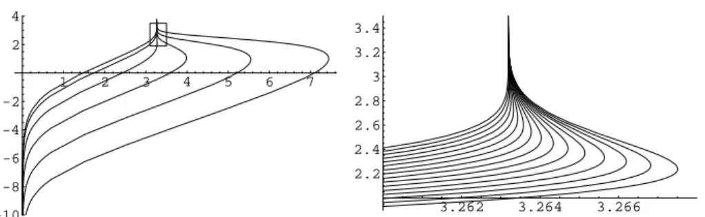
In Fig. 2, we recover that M (s) → 8 π as s → ∞. Moreover, for τ large enough, there are two solutions corresponding to a given M larger than 8 π, with M − 8 π not too large. Since it is of interest to decide for which values of τ solutions may have mass larger than 8 π, the small rectangle in Fig. 2 (left) is enlarged in Fig. 2 (right).
It can be numerically checked that solving the equations on (ε, rmax) with rmax= 10
gives a good approximation of the solution. Furthermore, here we took ε = 10−8 and s ∈ [−10, 20]. -25 -20 -15 -10 -5 5 -4 -3 -2 -1 1 2 3 4
Fig. 1 The set of all positive solutions of ∆vσ+ τ2ξ · ∇vσ+ σ evσe−|ξ|
2/4
= 0 in C2 0(R2), where σ = σ(s) = ew(∞;s), is represented by the multivalued diagram s 7→ (log σ, log v
σ(0)) for τ = 10α, α = −2, −1, . . . , 3. Recall that the solutions v
σare radial and decreasing so that vσ(0) = kvσkL∞(R2). We observe that max
s∈Rlog σ(s) appears as an increasing function of τ .
1 2 3 4 5 6 7 -10 -8 -6 -4 -2 2 4 3.262 3.264 3.266 2.2 2.4 2.6 2.8 3 3.2 3.4
Fig. 2 Left:The set of all positive solutions of ∆vσ+τ2ξ ·∇vσ+σ evσe−|ξ|
2/4
= 0 in C2 0(R2) is now represented by the diagram s 7→ (log(1+M (s)), log vσ(0)) for τ = 10α, α = −2, −1, . . . , 3. We observe that max
s∈RM (s) appears as an increasing function of τ .
Right:The plot is an enlargement of the rectangle of Fig. 2 (left), with τ = 0.60, 0.62, 0.64, . . . , 0.90. Numerically, the first solution with mass larger than 8 π appears for τ ∈ (0.62, 0.64), which is far below the bound found in Section 2. This is not easy to read on the above figure, but it can be shown graphically by enlarging it enough.
6.2 Cumulated densities
Plots and bifurcation diagrams of forward self-similar solutions can be computed in the framework of cumulated densities (29)–(30), (33). However, again one has to be careful with the singularity at the origin. As above, since for ε > 0 small enough, S′∼ φ′∼ a on (0, ε) and so
S(y) = a y + O(ε2) and φ′′(y) ∼ −a4(1 + 2 a) + O(ε) , we practically solve (29)–(30) on (ε, ymax) with the initial data
φ′(ε) = a −a
4(1 + 2 a) ε , φ(ε) = a ε − a
8(1 + 2 a) ε
2 and S(ε) = a ε .
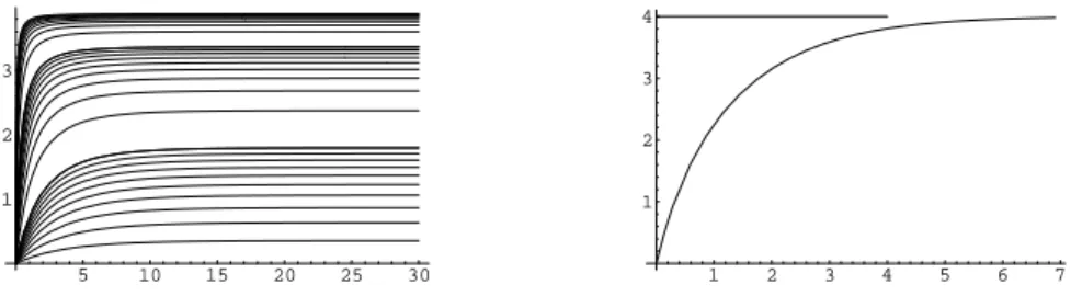
for any y ∈ (0, ε). Obviously, having fixed ε > 0, one has to take a in such a way that φ′(ε) − a = o(a). Here, we choose ε = 10−6. Finally, we shall approximate M from below by φ(ymax) with ymaxlarge enough. Figs. 3 and 4 correspond to the cases τ = 0.1
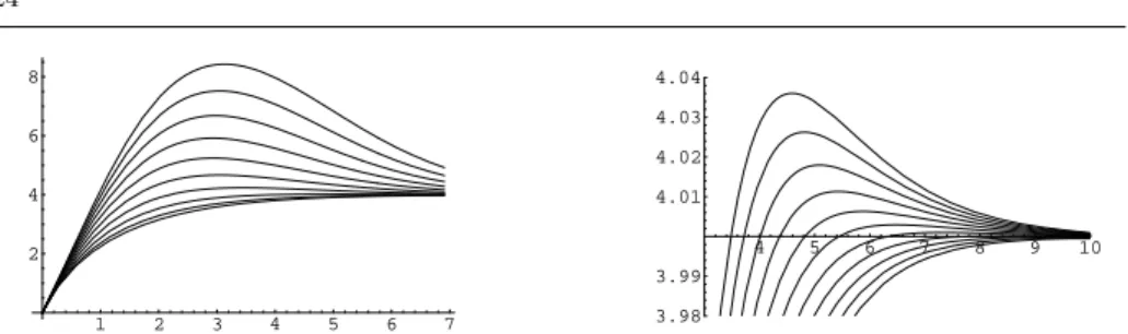
and τ = 10 respectively. For τ = 0.1, the value 8 π for the total mass is achieved only asymptotically in the limit a → ∞. For τ = 10, self-similar solutions with mass M larger than 8 π exist for a large enough. Finally, Figs. 5 and 6 show the total mass as a function of a and τ . 5 10 15 20 25 30 1 2 3 1 2 3 4 5 6 7 1 2 3 4
Fig. 3 Left: Plots of φ for φ′(0) = a, with a = 10bc, b = −1, 0, 1, c ∈ {1, . . . , 10} for τ = 0.1. Right: Plot of b 7→ φ(ymax) in the logarithmic scale, with φ′(0) = a, a = eb− 1, ymax= 30.
2.5 5 7.5 10 12.5 15 17.5 20 2 4 6 8 2 4 6 8 2 4 6 8
Fig. 4 Left: Plots of φ for φ′(0) = eα, with α = 1, 2, . . . , 20 for τ = 10. Right: Plot of φ(ymax) as a function of b (in the logarithmic scale), with φ′(0) = a, a = eb− 1. Here τ = 10, ymax= 30.
1 2 3 4 5 6 7 2 4 6 8 4 5 6 7 8 9 10 3.98 3.99 4.01 4.02 4.03 4.04
Fig. 5 Left: The value of mass φ(∞) = M (a, τ )/(2 π) in the logarithmic scale as a function of a, for τ = 0.1 k2with k = 1, 2, . . . , 10. Right: An enlargement around the value M (a, τ )/(2 π) = 4 in the logarithmic scale as a function of a, for τ = 0.50, 0.55, 0.60, . . . , 1.00.
0.5 0.6 0.7 0.8 0.9 4.005 4.01 4.015 4.02 4.025 4.03 4.035
Fig. 6 The value of the maximal (in terms of a) mass φ(∞) = M∗(τ )/(2 π) as a function of τ . Numerically, the first solution with mass larger than 8 π appears for τ ∈ (0.62, 0.64), as already noticed at the level of Fig. 2 (right). This is again not easy to read on the above figure, but it can be shown graphically by enlarging it enough.
7 Conclusions
Self-similar solutions are much more than an example of a family of solutions. The experience of various nonlinear diffusion equations shows that they are likely to be attracting a whole class of solutions, although this is still an open question for the parabolic-parabolic Keller–Segel model with large mass (see [14] for a result for small mass solutions). It is quite reasonable to expect that well chosen perturbations of these solutions asymptotically converge in self-similar variables to the stationary solutions we have found. This actually raises a much more interesting question, which is how to determine the basin of attraction of these self-similar solutions and to understand where is the threshold between solutions for which diffusion predominates and solutions which aggregate. Clearly, it is not going to be as simple as in the parabolic-elliptic case, where a single parameter, the total mass, determines the asymptotic regime. We can conjecture that blowup occurs for mass large enough and even, maybe, as soon as the total mass of the system is above 8 π if initial data are sufficiently concentrated.
The model considered in this paper is by many aspects ridiculously simple. See, for instance, [9] to get a taste of the variety of the nonlinearities that make sense even for a rather crude modelling purpose. Still, these models, in limiting regimes, asymptotically exhibit scaling properties similar to the ones of the parabolic-parabolic Keller–Segel model considered here. Therefore, we believe that the information gath-ered above, together with the methods that have been introduced, for instance, the cumulated densities reformulation of the model, should definitely be some valuable
piece of information in the study of the asymptotic behaviors of the equations used in chemotaxis.
Acknowledgements The authors have been supported by Polonium contract nr. 13886SG (2007–2008). This work has been initiated during the Special semester on quantitative biol-ogy analyzed by mathematical methods, October 1st 2007 – January 27th, 2008, organized by RICAM, Austrian Academy of Sciences, in Linz. More recently, this research has been partially supported by the ANR CBDif-Fr, the European Commission Marie Curie Host Fel-lowship for the Transfer of Knowledge “Harmonic Analysis, Nonlinear Analysis and Probabil-ity” MTKD-CT-2004-013389, and by the Polish Ministry of Science (MNSzW) grant – project N201 022 32/0902.
c
2009 by the authors. This paper may be reproduced, in its entirety, for noncommercial purposes.
References
1. Biler, P.: Local and global solvability of some parabolic systems modelling chemotaxis. Adv. Math. Sci. Appl. 8(2), 715–743 (1998)
2. Biler, P.: A note on the paper of Y. Naito: “Asymptotically self-similar solutions for the parabolic system modelling chemotaxis”. In: Self-similar solutions of nonlinear PDE,
Banach Center Publ., vol. 74, pp. 33–40. Polish Acad. Sci., Warsaw (2006)
3. Biler, P., Karch, G., Lauren¸cot, P., Nadzieja, T.: The 8π-problem for radially symmetric solutions of a chemotaxis model in the plane. Math. Methods Appl. Sci. 29(13), 1563–1583 (2006)
4. Blanchet, A., Carrillo, J.A., Masmoudi, N.: Infinite time aggregation for the critical Patlak-Keller-Segel model in R2. Comm. Pure Appl. Math. 61(10), 1449–1481 (2008)
5. Blanchet, A., Dolbeault, J., Perthame, B.: Two-dimensional Keller-Segel model: optimal critical mass and qualitative properties of the solutions. Electron. J. Differential Equations 44, 32 pp. (2006)
6. Brezis, H., Merle, F.: Uniform estimates and blow-up behavior for solutions of −∆u = V (x) eu in two dimensions. Comm. Partial Differential Equations 16(8-9), 1223–1253 (1991)
7. Calvez, V., Corrias, L.: The parabolic-parabolic Keller-Segel model in R2. Commun. Math. Sci. 6(2), 417–447 (2008)
8. Dolbeault, J., Perthame, B.: Optimal critical mass in the two-dimensional Keller-Segel model in R2. C. R. Math. Acad. Sci. Paris 339(9), 611–616 (2004)
9. Hillen, T., Painter, K.J.: A user’s guide to PDE models for chemotaxis. J. Math. Biol. 58(1-2), 183–217 (2009)
10. Horstmann, D.: On the existence of radially symmetric blow-up solutions for the Keller-Segel model. J. Math. Biol. 44(5), 463–478 (2002)
11. Horstmann, D.: From 1970 until present: the Keller-Segel model in chemotaxis and its consequences. I. Jahresber. Deutsch. Math.-Verein. 105(3), 103–165 (2003)
12. Mizutani, Y., Muramoto, N., Yoshida, K.: Self-similar radial solutions to a parabolic sys-tem modelling chemotaxis via variational method. Hiroshima Math. J. 29, 145–160 (1999) 13. Muramoto, N., Naito, Y., Yoshida, K.: Existence of self-similar solutions to a parabolic
system modelling chemotaxis. Japan J. Indust. Appl. Math. 17, 427–451 (2000) 14. Naito, Y.: Asymptotically self-similar solutions for the parabolic system modelling
chemo-taxis. In: Self-similar solutions of nonlinear PDE, Banach Center Publ., vol. 74, pp. 149–160. Polish Acad. Sci., Warsaw (2006)
15. Naito, Y., Suzuki, T., Yoshida, K.: Self-similar solutions to a parabolic system modeling chemotaxis. J. Differential Equations 184(2), 386–421 (2002)
16. Raczy´nski, A.: Stability property of the two-dimensional Keller–Segel model. Asymptotic Analysis 61, 35–59 (2009)
17. Tindall, M.J., Maini, P.K., Porter, S.L., Armitage, J.P.: Overview of mathematical ap-proaches used to model bacterial chemotaxis. II. Bacterial populations. Bull. Math. Biol. 70(6), 1570–1607 (2008)
18. Tindall, M.J., Porter, S.L., Maini, P.K., Gaglia, G., Armitage, J.P.: Overview of math-ematical approaches used to model bacterial chemotaxis. I. The single cell. Bull. Math. Biol. 70(6), 1525–1569 (2008)
19. Yoshida, K.: Self-similar solutions of chemotactic system. Nonlinear Analysis 47, 813–824 (2001)