A Compositional Approach to Robotic Impedance
Control
by
David Verdi
B.S., Columbia University (2017)
Submitted to the Department of Mechanical Engineering
in partial fulfillment of the requirements for the degree of
Master of Science in Mechanical Engineering
at the
MASSACHUSETTS INSTITUTE OF TECHNOLOGY
June 2019
@Massachusetts
Institute of Technology 2019. All rights reserved.
Signature redacted
A uthor ...
...
Department of Mechanical Engineering
May 14, 2019
Signature redacted
C ertified by ...
...
Neville Hogan
Sun Jae Professor of Mechanical Engineering
Signature redacted
Thesis Supervisor
A ccepted by ...
...
MASSACHUSETTS NSTITUTE
I
Nicolas G.
Hadjiconstantinou OFTECHNOLOGY PProfessor of Mechanical Engineering
JUN 13 2019
Chairman, Committee on Graduate Students
A Compositional Approach to Robotic Impedance Control
by
David Verdi
Submitted to the Department of Mechanical Engineering on May 14, 2019, in partial fulfillment of the
requirements for the degree of
Master of Science in Mechanical Engineering
Abstract
While the gap between robot and human performance is rapidly closing, humans still vastly outperform robots at dynamic interaction tasks, particularly those which involve manipulation into kinematic singularities, and those which might involve col-laborative or closed kinematic chain manipulation with multiple actuators. In this work, compositional impedance control, or linearly superimposing impedance con-trollers on a robot, is presented as a step towards closing this performance gap.
First, an overview of compositional impedance control is provided, along with a discussion of the control framework's applications to redundancy resolution, con-trolling closed kinematic chains, managing collaborative manipulation, and tackling high-DOF manipulation tasks. This control scheme was implemented on a Baxter Research Robot, and a series of system identification experiments were conducted to determine how well the robot was able to render the desired impedance parameters, and how well those parameters linearly superimposed between two arms collabora-tively manipulating an object. Commanded static stiffness was found to be delivered
by each individual arm to within a 2% error, while the linear superposition was
ver-ified to within 3% error. Commanded endpoint damping was found to be delivered
by the robot with a 17% and 57% error by the left arm and right arm respectively.
Linear superposition for damping was verified to within 7% error.
Using this compositional impedance control framework, sample manipulation tasks such as closed-chain manipulation into singularity, and high-speed closed-chain cloth manipulation (in the form of robotic shoeshining) were implemented. Finally, nullspace projection methods for redundant manipulators are discussed, and an impedance based implementation of the nullspace projection method is presented.
Thesis Supervisor: Neville Hogan
Acknowledgments
First and foremost I would like to thank my thesis advisor, Professor Neville Hogan for mentoring me throughout my graduate career at MIT. His knowledge of multi-domain system dynamics, control theory, and human motion control is unparalleled, and inspiring. It is truly an honnor to work alongside him, and I couldn't have asked for a better advisor.
I would also like to thank the graduate students and postdocs in the Newman Lab, especially James Hermus, Jongwoo Lee, Meghan Huber, Davi da Silva, Joe Davidson, Moses Nah, Logan Leahy, and Michael West. The innumerable, and extensive conver-sations on everything from the minute details of implementing eigenvector placement in a state-space control problem, to broader questions on our life trajectories greatly enriched my graduate experience.
Additionally, I would like to thank my professors and teaching assistants for tire-lessly holding me to the high standards that give MIT its reputation. My grasp and comfort with many topics in controls, system dynamics, and robotics has grown immensely because of it.
I also want to thank Professor Henry Hess at Columbia University for mentoring me for many years, and teaching me the importance of reasoning from first principles. I also want to thank Professor Kristin Myers at Columbia University, who helped me along the path to graduate school. I would also like to thank Michael Propper and Dr. Robert Muratore, both of whom sparked my interest in physics.
Finally, I want to thank my parents, my friends, and my family. I wouldn't have been able to do any of this without their endless support. I would also like to thank the fantastic communities at the MIT Sailing Pavilion, the MIT Coffeehouse Lounge (particularly on Saturday nights), MIT Hillel, MIT Chabad, and Harvard Hillel for making life in Cambridge so fun.
This research was performed in the Eric P. and Evelyn E. Newman Laboratory for Biomecahnics and Human Rehabilitation at the Massachusetts Institute of
Tech-nology. The research presented in Chapters 1 - 5 was supported by The National Science Foundation - National Robotics Initiative Grant No. 1637824. The research presented in Chapter 6 was supported by the Centers for Mechanical Engineering Re-search and Education at MIT and SUSTech, Project: Towards Whole-Body Physical
Contents
1 Introduction
1.1 Equivalent Networks and the Human Motion 1.2 Impedance Control in Robots . . . . 1.2.1 Overview . . . . 1.2.2 Controller Derivation . . . . 1.2.3 Advantages . . . . 1.3 Overview of Thesis . . . .
Controller
2 Compositional Impedance Control
2.1 The Linear Superposition Property . . . . 2.2 Redundancy Resolution . . . . 2.3 Closed Kinematic Chains . . . . 2.4 Collaborative Manipulation . . . . 2.5 Tackling the Scale Up Problem . . . . 2.5.1 Com plex Tasks . . . . 2.5.2 High-DOF Systems . . . .
3 Implementation on a Baxter Research Robot
3.1 Robot Hardware Overview . . . . 3.2 Robot Control Overview . . . . 3.3 High Level Impedance Controller Implementation Details . . . . .
4 Verifying Impedance Composition and Controller Performance
15 16 20 20 21 29 31 33 33 34 38 39 41 41 42 45 45 48 50 53
4.1 Overview and Methodology . . . . 53
4.2 Controller Settings . . . . 60
4.3 Static Stiffness Identification . . . . 61
4.4 Damping and Inertia Identification . . . . 62
4.4.1 Damping Parameter Fits . . . . 62
4.4.2 Inertial Parameter Fits . . . . 72
5 Sample Manipulation Tasks 75 5.1 Manipulation Into A Singularity . . . . 75
5.2 Complex Task Proof of Concept: Robotic Shoe Shining . . . . 76
6 Nullspace Projections: An Impedance Based Interpretation 83 6.1 The Traditional Approach . . . . 84
6.2 An Impedance Based Approach . . . . 91
6.3 Comparison of Projection Behavior at Singularity . . . . 94
6.3.1 Traditional Approach . . . . 95
6.3.2 Impedance Based Approach . . . . 95
7 Conclusions and Future Work 105 7.1 C onclusions . . . . 105
7.2 Future W ork . . . 107
7.2.1 System Identification of Back-Driving Impedances . . . . 107
7.2.2 Tackling the Optimization Scale Up Issue . . . . 110
7.2.3 Impedance Based Nullspace Projection Behavior at Singularity 111 A Expected Endpoint Stiffness, Damping, and Inertia Matrices for Sys-tem ID Experiments 113 A.1 Net Endpoint Stiffnesses . . . . 113
A.2 Net Endpoint Damping . . . . 114
A.3 Net Endpoint Inertia . . . . 115 B Motions Along y and z Coordinates During Step Responses 117
List of Figures
1-1 Th6venin and Norton Equivalent Circuits . . . . 17
1-2 Nonlinear Equivalent Network of the Human Acutator . . . . 19
1-3 1-D O F R obot . . . . 21
1-4 1-DOF Robot Under Impedance Control . . . . 22
1-5 1-DOF Robot Under Impedance Control With Damping to Ground . 23 1-6 4-DOF Planar Robot Operating in 3-DOF Planar Space . . . . 24
1-7 Behavior of a Planar Robot Under Impedance Control . . . . 26
2-1 Inertial Object With Nonlinear Impedance Elements . . . . 33
2-2 4-DOF Planar Robot . . . . 35
2-3 Superimposed Endpoint and Joint-Space Impedance Behavior . 36 2-4 Closed Kinematic Chain Manipulator . . . . 38
2-5 Closed Kinematic Chain Manipulator Under Impedance Control . . . 39
2-6 Collaborative Manipulators . . . . 40
2-7 Collaborative Manipulators Under Impedance Control . . . . 40
3-1 The Baxter Robot Joint Naming Convention and Internals . . . . 46
3-2 The Baxter Robot Dimensions and Coordinate System . . . . 47
3-3 Baxter Robot Torque Control Implementation . . . . 49
4-1 System ID Initial Pose . . . . 55
4-2 Aluminum Linkage Drawing . . . . 55
4-3 Baxter Robot With Linkage Installed . . . . 56
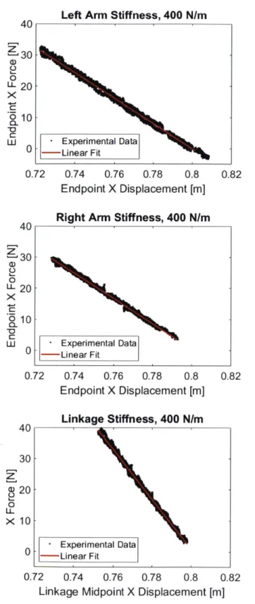
4-5 400 N/m Force vs. Displacement Stiffness Fits . . . . 64
4-6 400 N/m Force vs. Displacement Stiffness Fits . . . . 65
4-7 500 N/m Step Responses . . . . 67
4-8 400 N/m Step Responses . . . . 68
4-9 300 N/m Step Responses . . . . 69
5-1 Singularity Manipulation Task . . . . 76
5-2 Singularity Manipulation Trajectories . . . . 77
5-3 Jacobian Condition Numbers During Singularity Manipulation . . . . 77
5-4 Robotic Shoe Shining Task . . . . 79
6-1 Four Link Planar Robot Approaching Singularity . . . . 88
6-2 Jacobian Condition Number Approaching Singularity . . . . 89
6-3 Jacobian Pseudoinverse Norm Approaching Singularity . . . . 89
6-4 Three Link Planar Robot Approaching Singularity . . . . 95
6-5 Nullspace Projected Torques From the Traditional Method . . . . 96
6-6 Nullspace Projected Torques From the Traditional Method, With Ad-justed Zero Threshold . . . . 96
6-7 Eigenvalues of K O . . . . 97
6-8 Nullspace Torques From Impedance Method Without A Replacement 98 6-9 Nullspace Torques From Impedance Method With A Replacement At Singularity . . . . 99
6-10 Nullspace Projected Torques From the Impedance Based Method, With Adjusted Eigenvalue Zero Threshold . . . . 99
6-11 Eigenvector Contributions to Joint Torques . . . . 102
6-12 Eliminating Discontinuity by Ramping Up k2 . . . . 103
7-1 Two 1-DOF Robots . . . . 108
7-2 Two 1-DOF Robots Clamped Together . . . . 108
7-3 Two 1-DOF Robots Interacting . . . . 108
B-2 400 N/m Step Response y and z Displacements . . . . 119 B-3 300 N/m Step Response y and z Displacements . . . . 120
List of Tables
4.1 Nominal Endpoint Coordinates for System ID . . . . 54
4.2 Nominal Joint Angles for System ID . . . . 54
4.3 Results From Static Stiffness Identification Experiments . . . . 66
4.4 Results From Damping Identification Experiments . . . . 70
Chapter 1
Introduction
Robot performance has seen tremendous improvements over the past several decades. Nevertheless, humans still vastly outperform robots in tasks that involve complex dynamic interactions with the environment [Hogan, 2017, Krotkov et al., 2018]. For instance, a woodcarver might take a delicate workpiece with complex geometric fea-tures and proceed to scrub or sand its intricate contours. A painter might extend her arm to the edge of her dexterous workspace to carefully apply spackle to a difficult to reach location. A shoeshiner might stretch out a cloth between his hands and use it to rapidly buff a leather shoe.
In general, humans seamlessly transition from free to constrained motions, and can readily perform dynamic interaction tasks into and out of kinematic singularities. They easily manipulate a variety of compliant and non-compliant objects with two hands, or even coordinate large object manipulation with several other people. All of these tasks, while performed by humans with relative ease, can be challenging to program on a robot.
1.1
Equivalent Networks and the Human Motion
Con-troller
One source of inspiration for properly managing a robot's dynamic interactions with its environment is our current understanding of the human motion controller. The actual human neuromuscular physiology and control scheme is, of course, exceedingly complex, and our ability to study its internal details are currently quite limited [Kan-del et al., 2013]. One approach to gaining insight on the net interactive behavior of this "black box" is to borrow the idea of an equivalent network from circuit theory [Hogan, 2014, Hogan, 20171.
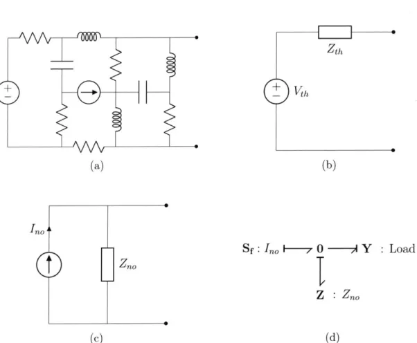
Given a complex circuit with an arbitrary number of interconnected sources and dynamic elements (such as resistors, inductors, capacitors, voltage sources, and cur-rent sources), we can exactly model the output port behavior of the circuit with a far simpler Norton or Th6vinin equivalent circuit, as depicted in Figure 1-1
[Horowitz
and Hill, 2015]. In the case of a Norton equivalent, the complex circuit is replaced by a controlled current source and parallel impedance, while in the case of a Th6venin equivalent, the complex circuit is replaced by a controlled voltage source and series impedance.In the electrical domain, the impedance of an element is defined as the functional relationship between the input current through the element (flow variable), and the output voltage across the element (effort variable):
V = Z{I} (1.1)
For instance, the constitutive equation of a resistor could be written as V = RI, that of a capacitor as V
J
f
Idt, and that of an inductor as V Cf = L . In the specialdt case of a linear element, the impedance relationship can be expressed as a transfer function in the Laplace domain:Z(s) = V(s) (1.2)
(a) (b Ino (c) Sf : Ino 1- 7 0 -- Y : Load ZnO Z : ZnO (d)
Figure 1-1: (a) A complex circuit with many interconnected dynamic elements and sources. (b) A Th6vinin equivalent circuit with a voltage (effort) source and series impedance. (c) A Norton equivalent circuit with a current (flow) source and par-allel impedance. (d) A bond graph representation of the Norton equivalent circuit, connected to a load modeled as an admittance.
(b)
...
IIIIIIIIIIIIIIIIIIIIJ
Zth
where s is the Laplace variable.
There exists a one-to-one mathematical analogy between the modeling of elec-trical system dynamics and mechanical system dynamics [Brown, 2001, Hogan and Breedveld, 2002]. The effort variable (voltage) becomes force, and the flow variable (current) becomes velocity. Similarly, resistance is analogous to viscous damping, capacitance is analogous to stiffness, and inductance is analogous to inertia, with all constitutive equations taking on an identical form. In the mechanical domain the impedance can be written as:
f
= Z{i} (1.3)However, the usual convention for mechanical systems is to write the impedance operator in terms of x rather than +. The encoded information is the same, but more potentially problematic differentiations may be required in the operator
[Brown,
2001]:f = Z{x} (1.4)
Finally, for a linear mechanical system, we can write:
Z(s) = Fs (1.5)
We can thus extend the ideas of Norton and Thevinin equivalent networks to the mechanical domain, which includes the human musculoskeletal system
[Hogan,
2014, Hogan, 2017].A block diagram of a Norton1 equivalent network for a human limb is shown in Figure 1-2. In addition to being competent enough to describe the full interactive dynamics of the limb, this model reflects key insights that we have gained about up-per limb motion control. Many findings suggest that the human motion controller specifies a nominal limb position (or trajectory) by setting the relative activation level of opposing antagonist muscle pairs [Feldman, 1966, Bizzi et al., 1982, Bizzi et al.,
'See [Hogan, 20171 and [Hogan, 20141 for a full discussion of why the Norton network, and not the Thevinin network, is the appropriate choice here. In brief, the Norton network is translation invariant (independent of our chosen coordinate frame), and its equivalent source is unambiguously identifiable.
CNS
Impedance Command , Equivalent Impedance, Z{ Ax} f
(Interactive Dynamics)Ineato
Interaction
CNS AX Port
Motion Command , Equivalent Xo +
-Motion Source E
Figure 1-2: A block diagram of a Norton equivalent network of the human motion control system. Here, the central nervous system provides a virtual trajectory xO and an effective hand impedance, Z{}. The difference between the virtual and actual hand position, Ax, along with the effective hand impedance determines the contact force that will be felt at the interaction port. Figure adapted from [Hogan, 2014].
1984]. For instance, the nominal elbow joint angle is moved and set by changing the ratio of activation between the elbow flexors (brachialis, biceps brachii, and the brachioradialis) relative to the elbow extensors (triceps brachii and anconeus) [Net-ter, 2014]. This trajectory, denoted as xO in Figure 1-2, is known as the reference trajectory, zero-force trajectory or virtual trajectory2, as it is the (potentially non-physically realizable) trajectory along which the hand would move in the absence of external forces or constraints. As long as the impedance operator is invertable, the virtual trajectory exists, regardless of whether the hand is performing free motion tasks, or constrained motion (contact) tasks
[Doeringer,
1999, Hermus, 2018].Another important aspect of human motion control that the model captures is the equivalent impedance at the hand, which is also set by commands from the central nervous system. Hand stiffness is adjusted by the central nervous system by either co-activating opposing antagonist muscle pairs [Humphrey and Reed, 1983, Hogan, 1984], or by modulating reflex gains in spinal cord feedback loops [Nichols and Houk, 1976, Hoffer and Andreassen, 1981]. While the intrinsic mass of the adult musculoskeletal system is fixed, the effective inertia felt in each direction at the hand is heavily dependent on the configuration of the arm [Hogan, 1990]. The combined impact of all of these factors determines the effective arm impedance, Z{-}. This effective impedance is what determines the interaction force felt when the arm is deflected from
2While these terms can denote different concepts in human motion control research, they are used interchangeably here in the context of robot control.
its virtual trajectory in a constrained motion task, or in response to a disturbance [Hogan, 2017]. For humans to successfully perform complex tasks, controlling this effective arm impedance is key [Burdet et al., 2001, Franklin et al., 2007, Schabowsky et al., 2007, Damm and McIntyre, 2008, Selen et al., 20091.
1.2
Impedance Control in Robots
1.2.1
Overview
Traditionally, many robot control frameworks involve tightly controlling a single set of manipulator variables [Spong and Vidyasagar, 1989]. These variables might be joint positions in the case of position control, endpoint forces in the case of force control, or a combination of endpoint positions and forces in orthogonal directions in the case of hybrid position/force control [Craig and Raibert, 1979, Raibert and Craig, 1981, Mason, 1981, Ortenzi et al., 2017]. These methods work perfectly well for many robot applications. Position control, for instance, is widely used for free space tasks such as pick-and-place or spray painting operations
[Gasparetto
et al., 20121, while force control is often used for interaction tasks, such as robotic deburring in structured industrial environments [Stepien et al., 1987].These traditional control algorithms are, however, not very versatile. For instance, force control is only usable in situations when the manipulator is guaranteed to be in contact with the environment, otherwise the manipulator will rapidly accelerate to the edge of its workspace. Even in situations where contact is guaranteed, the force control algorithm might still suffer from stability issues [Whitney, 1977, Colgate and Hogan, 1989a]. Position control, by contrast, is only usable in free space, since contact may cause damage to either the robot, or objects in the environment. It is possible to switch between position control and force control via a finite state machine when contact is detected, but this requires very accurate robot perception algorithms, and robust methods to deal with event detection uncertainties
[Salehian
et al., 2018, Atkeson et al., 2018].X
Fact
Fext
Figure 1-3: 1-DOF manipulator with mass m, actuation force Fact, and external force
Fex. All displacements and forces pointing to the right will be considered positive.
An alternative approach to robot control that is suitable for both free-space and contact tasks might look like our equivalent ietwork model of the human motion
control system in Figure 1-2. In this paradigm, we forego rigidly controlling a single
set of manpulator variables such as endpoint forces or positions. Instead, we shape the relationship between input flow variables (e.g. manipulator endpoint position or velocity relative to a reference trajectory) and output effort variables (e.g. net endpoint forces and torques) at an interaction point with the environment. By doing this, we are essentially shaping the effective impedance of the robot endpoint. This control technique was introduced by Hogan, and is called known as impedance control [Hogan, 1985a, Hogan, 1985b, Hogan, 1985c].
1.2.2 Controller Derivation
1-DOF Case
To elucidate the idea of impedance control, we can consider the case of a 1-DOF
actuated manipulator, with mass m, actuation force Fact, and an external force Fet, which represents either a directly applied disturbance force, or the interaction force that arises over the course of a contact or manipulation task. Such a manipulator is shown in Figure 1-3.
One simple impedance control implementation is to give a manipulator the appar-ent behavior of a mass-spring damper system (second order dynamics). The behavior
X0
X
k
0
Fext
b
Figure 1-4: A 1-DOF manipulator under an example simple second order impedance controller. All displacements and forces pointing to the right will be considered positive.
of this controller is visualized in in Figure 1-4. To implement this, we can use the control law:
Fact k(x0 - x) + b(i0 - (1.6)
where x0 is a reference (virtual) trajectory, k is the spring stiffness, and b is the viscous damping. This controller gives us the desired behavior in Figure 1-4. The disturbance response of the manipulator under this control law is:
Z Fet - os2 + bs + k (1.7)
X
where s is the Laplace variable. This is the effective endpoint impedance that char-acterizes the interactive behavior of the robot. The forward path dynamics of this controller are as follows:
X bs+k
X0 mos2 +bs+k
The forward path dynamics of this controller has a dynamic zero ats= - which
comes as a consequence of defining the damping relative to the reference trajectory,
xo. One important ramification of defining the damper this way is that in order for our control law (Eqn. 1.6) to be implemented, x0 must be differentiable. If we wish to maintain the system's desired interactive impedance (Eqn. 1.7), while also allowing us to use non-differentiable reference trajectories, we can define the damper relative to mechanical ground, as in Figure 1-5. This is particularly useful for system
X0
X
k
Fext
b
Figure 1-5: A 1-DOF manipulator under a simple second order impedance controller with damping defined relative to a fixed ground point. All displacements and forces pointing to the right will be considered positive.
identification purposes, where a non-continuous and non-differentiable step function
in x0 can be used. This controller is implemented as:
F,1 k(1o - )b(J) (1.9)
This controller has the forward path transfer function:
X_ k
X - k(1.10) Xo mos2 +bs + k
All of the above control laws do not attempt to modify the effective manipulator mass, mo. If we wish to do so, we can write a more advanced controller to replace our given mo with a desired Md [Hogan, 1985b, Hogan, 1987]. Assuming we have a measurement of the external interaction force Fet, we can implement the control law:
Fact = mo [k(xo - x) + b(o - )] + [MO- 1]Fext (1.11)
md md
which gives us the behavior shown in Figure 1-4, but with an arbitrary mass Md. Replacing io with zero will yield behavior analogous to that of Figure 1-5. One caveat to this approach is that incorporating force feedback into the control loop for apparent mass modification might be a source of instability, depending on the dynamics between the robot, sensors, and manipulated objects [Colgate and Hogan,
04 [aY,0
03
Figure 1-6: A 4-DOF manipulator operating in 3-DOF planar space. The
joint-space configuration variables are q =
[01
02 03 04]T, while the endpoint spatialcoordinates are x = [X y
#]
, where x and y represent Cartesian position, and#represents endpoint orientation.
1989a, Colgate and Hogan, 1989b, Newman, 1992].
Multi-DOF Case
We can extend the above analysis to a multi-DOF robot. Consider an n-DOF robot operating in m-DOF space. The configuration of this robot is given by a vector of generalized joint angles/positions q E Rn, and the spatial coordinates of the robot endpoint are given by a vector x E R'. These coordinates are referred to as either endpoint coordinates, or operational space coordinates. For robots operating in the real world, m = 6. If a robot has more degrees of freedom in its joint-space relative to its endpoint-space (n > m), the robot is known as a redundant manipulator. An example of a 4-DOF planar robot operating in 3-DOF planar space is given in Figure
1-6.
For a robot, the forward kinematics represents the unique mapping from joint space coordinates q to endpoint coordinates x
[Spong
and Vidyasagar, 1989]:x = L(q) (1.12)
This relationship is not, in general, uniquely invertible [Pieper, 1968]. The velocity kinematics of a robot is the mapping of joint space velocities q to endpoint velocities
+ [Spong and Vidyasagar, 1989]:
x==J4 (1.13)
where J =x aq n ER Xis the robot Jacobian matrix. The entries of this matrix are
usually nonlinear functions of q.
From the principle of virtual work, we obtain the mapping between joint torques and endpoint forces3 as follows [Spong and Vidyasagar, 19891:
_r = JT
f
(114where r E R" is the vector of generalized joint torques/forces, and
f
c R" is the vector of generalized endpoint forces/torques.The natural dynamics of a robot (neglecting friction and other possible non-conservative forces) are given in joint-space by the manipulator equation [Spong and Vidyasagar, 1989]:
Mgq +C4+ g = ract + JTfext (1.15) Here, Mg E R nX" is the robot joint-space inertia matrix, whose entries are usually nonlinear functions of q. C E Rn"" is the Coriolis matrix, whose entries are usually nonlinear functions of q and 4. g E R' is the vector of gravitational torques, whose entries are usually nonlinear functions of q. Tact E Rn is the vector of joint actuator
torques, and fext c R' is the vector of external/interaction forces applied on the
robot by the environment.
In our example system in Figure 1-6, we wish to implement a simple second order impedance controller such that the system will behave as a mass-spring-damper system (as in Figure 1-4), but along each of the coordinates in x. This desired behavior is illustrated in Figure 1-7. In essence, we wish to replace the natural
3
As is standard in the robotics literature, the term "joint torques" is a generalized term used to refer to both forces and torques in the joint space (torques about revolute joints, and forces on prismatic joints). Similarly, the term "endpoint forces" also refers to forces in linear coordinates, and torques along rotational coordinates. The 6 x 1 vector of generalized endpoint forces in robots operating in the real world is sometimes referred to as the "endpoint wrench"
XO [zy,q<]
Mx,d
yoi
Figure 1-7: The desired behavior of a planar manipulator under impedance control. The system behaves like a mass-spring-damper system along each coordinate in x.
dynamics of the robot (Eqn. 1.15) with:
Mxz + Ki(X -xo) + BX(i -O) = fext (1.16)
Here, Mx,d E R"X"' is the desired endpoint-space inertia matrix, K1 E R"X"' is
the desired endpoint-space stiffness matrix, and Bx E R"'X is the desired endpoint viscous damping matrix. Usually, we would like the mass-spring-damper systems along each coordinate in x to be decoupled from one another. In this case, the matrices Mx1 , K, and Bx would all be diagonal, and the entries would represent
the inertia, stiffness value, and damping value along each direction in x. There are
times, however, where off-diagonal couplings between endpoint coordinates may be
desirable [Hogan, 1985b].
[Hogan, 1987] provides a control law to replace the dynamics in Eqn. 1.15 with those of Eqn. 1.16. First, using the force-torque mapping in Eqn. 1.14, we can transform the actuator torques from joint space torques into endpoint forces. Eqn.
1.15 becomes:
Mq + C4 + g = JT(fact + fext) (1.17) Since Mi is a mass matrix, it is guaranteed to be positive definite and therefore invertible. Thus, we can solve for 4:
Recalling our velocity kinematics:
x=J4 (1.19)
If we differentiate this relationship with respect to time, we have:
x= Jid + j (1.20)
Substituting Eqn. 1.20 into Eqn. 1.18 and rearranging yields:
x = JM-1JT(fact+fext)- JM--[C4+g]+jq (1.21)
Here, we can touch upon the relationship between the joint-space inertia matrix of a manipulatorMq, and the endpoint-space inertia matrix of a manipulator Mx
[Hogan,
1987, Khatib, 1987, Khatib, 19951:
M;1 = JMq-1JT (1.22)
Substituting into Eqn. 1.21:
X = M1(fact + fext) - JMq-1 [C4 + g] + j4 (1.23)
Now, we solve for fact:
fact = Mx (2 + JMq-I [C4+ g - i4] - fext (1.24) This equation gives us the actuator forces that must be applied to the robot in order realize any desired trajectory, z, with all modeled robot dynamics compensated for. If we recall, our desired manipulator behavior under impedance control was given by Eqn. 1.16. Writing this in terms of a desired x:
We now substitute
zd
from Eqn. 1.25 intoz
from Eqn. 1.24:fact = MxM-[Kx(xo - x) +
Bx(.0-+ M [JM 1[C4 + g] - j4] (1.26)
+[MxM- - I] fext
where I is the identity matrix. We can multiply this equation by jT to transform
fact back to actuator joint-space torques to yield the control law:
Tact = JTMxM-' [Kx(xo - x) + Bx(0 -
]
+ JTM[JM j-'[C4 + g) - j4] (1.27)
+JT [MXM- 1 - I]fest
This is the multi-DOF equivalent of Eqn. 1.11, with the same stability caveats of incorporating force feedback into the control loop
[Colgate
and Hogan, 1989a, Colgate and Hogan, 1989b, Newman, 1992].We can apply several simplifications to this controller. First, if gravity compen-sation is included in a lower level of the robot control stack, we can neglect the gravitational torque vector (g = 0). Next, if the manipulator is moving slowly, we
can neglect the Coriolis term (C4 = 0) and the Jacobian derivative term
(j4
= 0). This eliminates the entire second line of Eqn. 1.27. The forces arising from these terms will now be treated as external disturbances to the controlled system.If the user does not wish to modify the robot's endpoint inertia matrix, we can setM ,d M. This sets the term MxM-j = I, which simplifies the first line, and
eliminates the third line of the equation, along with the need to incorporate force feedback into the loop. This will be the approach taken for the remainder of this work.
Our simplified controller thus becomes:
In a robot, we usually have accurate measurements of q and 4. Through the for-ward kinematics and velocity kinematics, our knowledge of q and 4 gives us accurate measurements of x and for incorporation into the controller:
Tact JT [Kx(xo - L(q))+ Bx(0 - J4)] (1.29)
This control law effectively "programs in" the impedance form of the constitutive equations of an operational space spring-damper system at the endpoint of the robot. The impedance control framework is, however, more general than this. We can im-plement any operational space equivalent dynamic behavior at the endpoint of the robot, as long as it can be described in the form of Eqn. 1.4 [Hogan, 1985c]. The torque control law would look like:
ract = jT [Z{x, X0 , ...
}]
(1.30)where Z can depend on an arbitrary number of system states or fixed parameters. We are of course, always free to add in inertial and Coriolis force compensation as in Eqn 1.27. One example application of this might be obstacle avoidance in the environment. We can define a three-dimensional nonlinear impedance field in the environment, with a unilateral non-linear repulsive potential (e.g. non-linear one-way spring force and state-dependent damping) being defined in the immediate vicinity of perceived objects in the robot's work space [Hogan, 1985c, Khatib, 1986, Newman and Hogan, 1987].
1.2.3
Advantages
The control law in Eqn. 1.29 has many favorable attributes from a robot control perspective. For instance, it allows us to control the endpoint trajectory of the robot
by directly specifying x0, without the use of any inverse kinematics. This is a highly
desirable quality since for many robotic manipulators, the inverse kinematics are difficult to compute in closed form (and thereby require a nonlinear optimization
approach, which is not guaranteed to converge), and are non-unique (in the case of a redundant manipulator, there are infinitely many solutions for the inverse kinematics) [Goodwine, 2004].
Many operational space controllers heavily depend on computing the inverse of the Jacobian matrix inside the control loop [Khatib, 1987, Raibert and Craig, 1981, Miomir et al., 2008]. This becomes problematic when the manipulator is commanded into a singular configuration (i.e. at the edge of the manipulator workspace), since the Jacobian rapidly loses rank and becomes ill-conditioned near singularities. This method, however, does not depend on any Jacobian inverse operations, and therefore is able to seamlessly venture into and out of singular configurations without any numerical instabilities.
Another advantage of this control law is that it is suitable for both manipulation tasks in free space, and in contact with the environment [Hogan, 1985c, Hogan, 1987]. This is in contrast to the aforementioned position control and force/hybrid control paradigms. In free space, the robot behaves as if the endpoint was under a compliant position controller, with inertial lag (i.e. x 0 will tend to lead x due to the inertia
of the robot). When the manipulator is brought into contact with the environment (i.e. when the virtual trajectory xo dips below the surface of a rigid object in the environment) the robot simply comes into contact with the object and applies a contact force. The magnitude and direction of the applied contact force can be controlled by modulating the Kx gain, or by adjusting how deeply x0 penetrates into
the object.
One final advantage of the impedance control framework is the ability to linearly superimpose a number of arbitrary non-linear impedance controllers onto a single robot manipulator [Hogan, 1985c]. This allows us to compose a number of differ-ent impedance controllers on a robot to achieve tasks such as redundancy resolution, closed kinematic chain manipulation, collaborative manipulation, and to tackle com-plex tasks involving many degrees of freedom. The compositionality property of impedance controllers will be the primary focus for the remainder of this work.
1.3
Overview of Thesis
This introductory chapter has provided the foundation for understanding robot impedance control in terms of its biologically inspired origins, implementation details, and ad-vantages over more traditional robot control approaches.
Chapter 2 delves into the compositionality property of impedance controllers. Applications to redundancy resolution, closed kinematic chains, collaborative manip-ulation, and scaling up to many degrees of freedom are discussed.
Chapter 3 discusses the particulars of implementing the impedance controller on a Baxter Research Robot, including high and low level control loop details, and the quaternion representation of rotational stiffnesses for numerical stability.
Chapter 4 discusses system identification performed on the Baxter Research Robot to verify how well multiple impedances linearly superimpose in practice, as well as to evaluate how well a commanded endpoint stiffness and damping can be realized at the robot endpoint.
Chapter 5 examines proof of concept tasks such as manipulating the robot into and out of singularities under impedance control, and also the application of the compositional impedance control method to a complex task, such as robotic shoe shining.
Chapter 6 discusses traditional nullspace projection techniques for controlling ma-nipulator redundancies (such that the redundancy resolution criteria does not impact the operational space task), as well as a new approach to generating a nullspace pro-jection operator, based on the kernel of the operational-space stiffness matrix reflected
into joint-space.
Finally, Chapter 7 discusses the conclusions of the present work, along with future directions for further inquiry on the subject at hand.
Chapter 2
Compositional Impedance Control
2.1
The Linear Superposition Property
One important property of impedance controllers is the ability to linearly superimpose
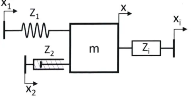
them in a robot [Hogan, 1985c]. To elucidate this idea, we consider an inertial object of mass m. Let us first attach a nonlinear spring, referenced to a virtual trajectory x1, with the constitutive equation
fi
= Zi{x,xi} = kX2(XI- x) . Next, let usattach a nonlinear damping element, referenced to a virtual trajectoryx2, with the
constitutive equation
f
2 = Z2{X, X2}= bsgn(iz2 - (- )2. Finally, let us attach ageneral nonlinear dynamic element with the constitutive equation
fi
= Zi{x, xi, ...}.
This arrangement is visualized in Figure 2-1.For N arbitrary nonlinear dynamic elements attached to the mass, Newton's
sec-X1aX
ZiZ
Z2 m -Z
X2
ond law yields:
N
mz = Zi{x, xI} + Z2{x, X2} + ... + ZNX, XN} i{X, Xi (2.1) i=1
Thus, we see that the net impedance (or net force) of a set of non-linear impedances acting on an inertial object is the linear superposition of those non-linear impedances. We can observe the same behavior for impedance controllers acting on a robot (which is fundamentally a set of inertial linkages). Given a set of N nonlinear endpoint-space impedance controllers that we would like to apply to a robot, our control law would be:
N
ract = JT Zi{x,1x}] (2.2)
i=1
We can also include impedances relative to any arbitrary coordinate system, as long as we have a Jacobian matrix that maps the joint-space coordinates to the new coordinate system. Finally, we can also add in M joint-space impedances into this framework as well (the Jacobian for this transformation is, of course, the identity matrix):
N M
Tact = JT[ Zix,
xz}]
+ Zj~q, qj} (2.3)i=1 j=1
2.2
Redundancy Resolution
One application of this linear superposition principle is redundancy resolution. Con-sider our example planar manipulator (reproduced in Figure 2-2). Since this robot has more joint-space degrees of freedom than endpoint degrees of freedom
(n >
m), it is a redundant manipulator. This means that the joint angles can be actuated continuously without impacting the position or orientation of the endpoint.To better understand this, we first recall the velocity kinematics of the robot (Eqn. 1.13). Here, the m x n Jacobian matrix maps the n-dimensional joint-space velocity
04
[XI
Y1
0]0:3
01
Figure 2-2: A 4-DOF planar robot. In this example, n= 4 and m= 3
vector to the m-dinensional endpoint-space velocity vector. If we assume the robot
is not in a singular configuration, the rank of the Jacobian is m (full row rank). Thus,
we see that the Jacobian has a null space with n - m basis vectors. Any joint space
velocity vector 4 in this null space will cause no motion in i, and will therefore not be impacted by the endpoint impedance controller (Eqn. 1.29). Consequently, small disturbance forces in the joint space of the robot can cause large, uncorrected motions in the joint-space.
To counter this, we can add a second impedance controller that operates in the joint space of the robot. A simple controller might specify a small stiffness about a nominal joint-space pose, q0, along with a small joint-space damping. This controller
has the form:
Tact =Kq(qo - q) - Bq(4) (2.4)
Here, Kq E R"X is the desired
joint-space
stiffness matrix, and Bq E R"" is thedesired joint-space viscous damping matrix. These matrices are usually diagonal, in which case the entries correspond to independent virtual rotational springs and dampers placed at each joint of the robot. The final control law is simply the sum of the two impedance controllers:
Tact = JT [Kx(xo - L(q)) + Bx(50 - J4)] + Kq(qo - q) - Bq(4) (2.5)
MX
0
YO
Figure 2-3: The effective behavior of a planar manipulator under a superimposed
endpoint and joint-space control law, as in Eqn. 2.5.
work. With this controller, all disturbances in the joint space will be met with a restoring force to bring the manipulator back towards its nominal joint space
config-uration. The effective endpoint of this control law is visualized in Figure 2-3.
One drawback of this method is that the effective endpoint stiffness and damping is no longer completely described by K, and B2. Instead, there is also some contribution to the endpoint stiffness and damping behavior from the small virtual springs and dampers that were placed at the robot joints. To analyze the net endpoint impedance behavior, we can map the joint-space stiffness matrix into endpoint-space.
For a robot, the map from a full-rank joint-space stiffness matrix Kq to an endpoint-space stiffness matrix B, is given by
[Mussa-Ivaldi
and Hogan, 1991]:K (J(K - T )-1jT)-l (2.6)
Here F is the kinematic stiffness term, which is given by:
F =
f
(2.7),9q
If we evaluate the system about zero endpoint force, the effective endpoint-space stiffness matrix becomes:
Kx|f=0 = (JKq-1JT (l (2.8)
space damping matrix is given by:
BX = (JB - JT)-- (2.9)
Note that these relationships are only valid when the manipulator Jacobian is of full row rank. In singular configurations (where the Jacobian loses rank), the endpoint stiffness and damping become unbounded in certain directions, since arbitrarily large forces applied in those directions will yield no motion. In contrast, the endpoint compliance matrix (the inverse of the endpoint stiffness matrix), and the inverse of the endpoint damping matrix, are both well defined quantities, and will go to zero in certain directions (instead of becoming unbounded) at singular configurations [Hogan,
1985b]. However, since stiffness and damping are more familiar properties to most
readers, those parameters, rather than their inverses, will be used in this work. From Eqns. 2.8 and 2.9, the net endpoint-space stiffness and damping matrices for the control law given in Eqn. 2.5 are:
Kx,nelf = Kx + (JK--i JT)l (2.10)
Bx,net B + (JBq-- JT)-l (2.11)
Another drawback of adding in a joint-space impedance to manage redundancies is that if qo remains fixed, there will be increasing steady-state errors in positioning if xO is driven far away from L(qo). In real systems, this can be mitigated by keeping Kqvery small compared to K, or by periodically re-adjusting qO to the current joint positions (this approach to mitigating positioning errors was not pursued further in this work).
An alternate approach would be to use null-space torque projections to ensure that the torques generated by the joint-space stiffness controller never produce any torques at the robot endpoint [Dietrich et al., 2015, Khatib, 1987, Khatib, 1995, Siciliano and Slotine, 1991]. These projections, along with their advantages and disadvantages will be discussed in Chapter 6.
Figure 2-4: A closed kinematic chain manipulator. For simplicity, we can assume that the first three joints of each sub-chain are actuated.
2.3
Closed Kinematic Chains
The idea of impedance composition can also be used to control closed kinematic chain manipulators, such as that shown in Figure 2-4. One way to control these robots is to "cut" the closed kinematic chain into two sub-chains at an un-actuated joint, and use position control techniques to place each subchain endpoint at the desired location [Siciliano et al., 2010]. In addition to the restrictions of position control mentioned in Section 1.2.1, one additional problem is that any imperfections in the kinematic model of the robot (e.g. from manufacturing tolerances or base coordinate system measurement error) will give rise to large, and possibly unacceptable internal forces on the distal link of the closed chain.
An alternative way of controlling this closed kinematic chain mechanism is via impedance control. In the case where every sub-chain is fully actuated or redundantly actuated, we can place the endpoint of each sub-chain under impedance control. The effective behavior of this controller is visualized in Figure 2-5. The net impedance behavior at the manipulator endpoint is again the sum of the two individual chain endpoint-space impedances. Additionally, this directly gives us endpoint space control without any inverse kinematic operations. This method also naturally lends itself to superimposing additional impedances for tasks such as collision avoidance.
IU0
Figure 2-5: The effective behavior of a closed kinematic chain manipulator with each sub-chain under impedance control.
2.4
Collaborative Manipulation
Another (similar) application of impedance control is to simplify collaborative manip-ulation between multiple robots, as in Figure 2-6. One traditional way of doing this is with a master-slave manipulation paradigm, where one robot (called the master) operates under endpoint position control mode to dictate the 6-DOF positioning of the object, while all of the other robots operate in force control mode to regulate the internal forces in the object
[Kosuge
and Hirata, 2004, Caccavale and Uchiyama, 2016, Nakano et al., 1974, Luh and Zheng, 1987]. Since this method may put undue burden on the master manipulator to handle most of the load, one can implement hybrid position/force control on all of the cooperative manipulators to divide the po-sitioning and force regulation tasks between them [Kosuge and Hirata, 2004, Hayati, 1986, Uchiyama and Dauchez, 1988]. These methods, while immensely useful, can be sensitive to kinematic modeling errors within and between the robots, and are not robust enough to handle situations where contact might be lost. Additionally, these control methods would not be suitable for situations where the commonly ma-nipulated object must be brought into or out of contact with other objects or rigid constraints in the environment.Impedance control provides an alternative way to handle the collaborative manip-ulation problem [Kosuge and Hirata, 2004, Koga et al., 1992]. In this case, we place both robot endpoints under impedance control, and the manipulated object behaves as if it is suspended by a set of mass/spring/damper systems, as in Figure 2-7. Here,
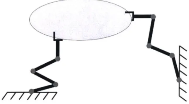
Figure 2-6: An example of two robots collaboratively manipulating an object
MX
Yoi
Figure 2-7: Impedance controllers on each collaborative manipulator makes the object behave as if it were suspended by a set of spring-damper systems
any errors in manipulator or object kinematics will only cause small deflections in the virtual springs at each robot endpoint, and will not result in large object inter-nal forces. Additiointer-nally, if tensile or compressive forces are desired in the object, they can be exerted by coordinating the equilibrium points of the multiple manip-ulators in contact with the object. One further advantage of this paradigm is that the system remains stable even if an individual manipulator loses contact with the object. The robustness inherent in this method of manipulator coordination makes it particularly suitable for manipulation in uncertain environments, manipulation of poorly modeled, delicate, flexible, or compliant objects (such as cloths), or manip-ulation with low-cost robots, which may have relatively large uncertainties in their kinematics due to manufacturing tolerances and variability. As noted in the previous section, the impedance composition method also allows for secondary impedances to be superimposed to handle tasks such as collision avoidance.
2.5
Tackling the Scale Up Problem
2.5.1
Complex Tasks
Managing complex manipulation tasks requires balancing and satisfying many differ-ent task requiremdiffer-ents. One example of a complex robotic manipulation task might be to rapidly buff a shoe using a cloth outstretched between two robotic manipulators. This is a task that humans can do with relative ease, but might pose a challenge to implement on a set of redundant robotic manipulators. In order to perform this task, the two robotic arms must first pick up a cloth, apply tension to the cloth without snapping it, bring the cloth above the shoe, bring the cloth into contact with the shoe, maintain a reasonable level of normal force on the shoe along with a reasonable amount tension in the cloth, and finally apply rapid oscillatory motions on the cloth to achieve a buffing effect.
If this is to be done with two 7-DOF manipulators, the task would require the coordinated motion of 14 degrees of freedom in a closed kinematic chain configuration incorporating the contact dynamics of a cloth, which are usually not trivial to model
[Yamakawa et al., 2011, Bai et al., 2016].
This is an example of a complex problem that is made far simpler by using a compositional impedance programming approach. First, the two robot manipulators would grip a slackened rectangular cloth, with one gripper on each end of the cloth.
Next, a set of endpoint-space virtual spring-dampers would be applied to the end effectors to gently pull the arms apart and apply outward tension on the cloth. Next, with the shoe placed under the cloth, a second set of spring-dampers would be applied to draw the cloth downwards to apply a normal force to the shoe. Finally, a third set of stiff spring-dampers would be applied with an oscillatory reference trajectory xo to rapidly draw the cloth back and forth over the shoe. Throughout the process, an-other set of small joint-space impedances would be applied to manage the redundant degrees of freedom in the robot. Due to the built-in controller compliance, a detailed computational model of the cloth and shoe are not necessary; an approximate mea-surement of the cloth length and shoe position will suffice. An implementation of this
strategy on hardware is given in Chapter 5.
The strategy here was to divide a complex task into smaller sub-tasks, and to devise an impedance controller to handle each sub-task or requirement. Additionally, we can sometimes rely on manipulator compliance in lieu of developing more pre-cise (and therefore computationally complex) models of the manipulated object and environment.
2.5.2
High-DOF Systems
Another challenge that compositional impedance control may be poised to tackle is that of controlling high-DOF systems. This may include modern humanoid robots, which may have 28 DOF in the case of Boston Dynamic's Atlas, 44 DOF in the case of NASA's R5 Valkyrie, or as many as 58 in the case of NASA's Robonaut 2 [Boston Dy-namics, 2019, Paine et al., 2015, NASA, 2014]. Controlling these high-DOF systems is a challenge, since the dynamics are nonlinear, and in the case of walking humanoid robots, underactuated [Tedrake, 2019]. One common approach to tackling this control problem is to perform large scale model predictive control (MPC)/nonlinear program-ming (NLP) to solve for a feasible torque trajectory subject to the system dynamics as constraints to the optimization problem, and a (usually) quadratic objective function to minimize [Betts, 1998, Tedrake, 2019]. While these methods scale well for a small to moderate number of degrees of freedom, the computational complexity causes it to fail for high-DOF systems [Kuindersma et al., 2014, Valenzuela, 2016, Betts, 19981. While progress can be made by linearizing the instantaneous dynamics at each opti-mization iteration, thereby converting the problem into a quadratic program
(QP),
the task still remains challenging
[Kuindersma
et al., 2014].As mentioned previously, one of the promises of the compositional impedance control method is the ability to divide a complex interaction task into a number of sub-tasks, and to fabricate an impedance controller for each one. If an impedance approach is suitable for a manipulation scenario involving a high-DOF system, we can identify sub-tasks and use optimization methods to aid in the design of impedance controllers for each one of those sub-tasks. In this manner, we would be solving several
lower dimensional NLPs, rather than one large scale NLP (which may not converge, or whose solution may be heavily dependent on the decision variable initializations) [Valenzuela, 2016].
Chapter 3
Implementation on a Baxter Research
Robot
3.1
Robot Hardware Overview
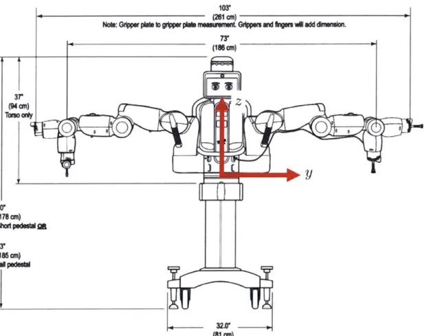
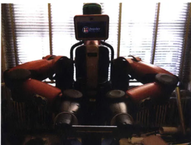
All of the experiments in compositional impedance control were performed on a Baxter Research Robot, which was manufactured by (the now defunct) Rethink Robotics (Boston, MA). The Baxter Robot is a low-cost anthropomorphic humanoid robot with two 7-DOF arms. A visualization of the robot joint naming convention, along with an image of the robot arm internals is given in Figure 3-1. A dimensioned drawing of the overall dimensions of the robot, along with the coordinate system is given in Figure 3-2.
Each joint contains a motor with a peak torque of 50 Nm for the shoulder and elbow joints, and 15 Nm for the wrist joints
[Rethink
Robotics, 2015g]. Each motor has the output of its gearbox connected to a relatively stiff series elastic element (843 Nm/rad on shoulder/elbow joints, and 250 Nm/rad on wrist joints), which allows for torque measurement and torque control at all joints [Rethink Robotics, 2015d, Re-think Robotics, 2015g, Hosford, 2016]. While each joint has a 14 bit encoder (yielding a 0.02° resolution), joint-level non-linearities yield a typical accuracy on the order of ±0.100 [Rethink Robotics, 2015g]. This, combined with manufacturing tolerances, yields a ±5 mm endpoint-space positioning accuracy while in position control modeEl EO Wo W2 -so W2 --) 'U
Figure 3-1: The image on the left shows a Baxter Robot arm with its cover removed. Here, one can see the joint motors, series elastic elements, and joint control boards. On the right is the joint naming convention. As this is an anthropomorphic robot, "S" stands for shoulder, "E" stands for elbow, and "W" stands for wrist. Images are adapted from [Knight, 2013] and [Rethink Robotics, 2015g]
103' (261 cm)
Nob:Gdpr pa ID gd pl mesmnmnt Gdesanmd ipnu m odd dmnion. r (18(cm) (94 cON TOWoenly 73-(178 cm) 7r (186 cm) Td piduM 3Wf (81 cm)
Figure 3-2: The overall dimensions of the robot, and the robot's cartesian coordinate system. The origin is located on the plane where the robot body is mounted to the pedestal. The positive x axis points out of the page. Image modified from [Rethink Robotics, 2015i].