Variability of the ocean heat content during the last millennium – an assessment with the ECHO-g Model

(1)

HAL Id: hal-03209347

https://hal.archives-ouvertes.fr/hal-03209347

Submitted on 28 Apr 2021

HAL is a multi-disciplinary open access

archive for the deposit and dissemination of

sci-entific research documents, whether they are

pub-lished or not. The documents may come from

teaching and research institutions in France or

abroad, or from public or private research centers.

L’archive ouverte pluridisciplinaire HAL, est

destinée au dépôt et à la diffusion de documents

scientifiques de niveau recherche, publiés ou non,

émanant des établissements d’enseignement et de

recherche français ou étrangers, des laboratoires

publics ou privés.

millennium – an assessment with the ECHO-g Model

P. Ortega, M. Montoya, F. González-Rouco, H. Beltrami, D. Swingedouw

To cite this version:

P. Ortega, M. Montoya, F. González-Rouco, H. Beltrami, D. Swingedouw. Variability of the ocean

heat content during the last millennium – an assessment with the ECHO-g Model. Climate of the Past,

European Geosciences Union (EGU), 2013, 9 (2), pp.547-565. �10.5194/cp-9-547-2013�. �hal-03209347�

(2)

Clim. Past, 9, 547–565, 2013 www.clim-past.net/9/547/2013/ doi:10.5194/cp-9-547-2013

EGU Journal Logos (RGB)

Advances in

Geosciences

Open Access

Natural Hazards

and Earth System

Sciences

Open Access

Annales

Geophysicae

Open Access

Nonlinear Processes

in Geophysics

Open Access

Atmospheric

Chemistry

and Physics

Open Access

Atmospheric

Chemistry

and Physics

Open Access Discussions

Atmospheric

Measurement

Techniques

Open Access

Atmospheric

Measurement

Techniques

Biogeosciences

Open Access Open Access

Biogeosciences

Discussions

Climate

of the Past

Climate

of the Past

Discussions

Earth System

Dynamics

Earth System

Dynamics

Discussions

Geoscientific

Instrumentation

Methods and

Data Systems

Open Access

_{Geoscientific}

Instrumentation

Methods and

Data Systems

Geoscientific

Model Development

Geoscientific

Model Development

Discussions

Hydrology and

Earth System

Sciences

Open Access

Hydrology and

Earth System

Sciences

Ocean Science

Discussions

Solid Earth

Discussions

The Cryosphere

Discussions

Natural Hazards

and Earth System

Sciences

Open Access

Discussions

Variability of the ocean heat content during the last millennium –

an assessment with the ECHO-g Model

P. Ortega1, M. Montoya1,2, F. Gonz´alez-Rouco1,2, H. Beltrami3, and D. Swingedouw4

1_{Dpto. Astrof´ısica y Ciencias de la Atm´osfera, Facultad de Ciencias F´ısicas, Universidad Complutense de Madrid, Spain} 2_{Instituto de Geociencias (UCM-CSIC), Madrid, Spain}

3_{Climate and Atmospheric Sciences Institute/Department of Earth Sciences, St. Francis Xavier University,}

Antigonish, Canada

4_{LSCE/IPSL Laboratoire des Sciences du Climat et de l’Environnement, CEA-CNRS-UVSQ – UMR8212, Gif sur Yvette,}

France

Correspondence to: P. Ortega (pablo.ortega@lsce.ipsl.fr)

Received: 30 July 2012 – Published in Clim. Past Discuss.: 30 August 2012 Revised: 5 February 2013 – Accepted: 7 February 2013 – Published: 4 March 2013

Abstract. Studies addressing climate variability during the

last millennium generally focus on variables with a direct in-fluence on climate variability, like the fast thermal response to varying radiative forcing, or the large-scale changes in at-mospheric dynamics (e.g. North Atlantic Oscillation). The ocean responds to these variations by slowly integrating in depth the upper heat flux changes, thus producing a delayed influence on ocean heat content (OHC) that can later im-pact low frequency SST (sea surface temperature) variability through reemergence processes. In this study, both the ex-ternally and inex-ternally driven variations of the OHC during the last millennium are investigated using a set of fully cou-pled simulations with the ECHO-G (coucou-pled climate model ECHAMA4 and ocean model HOPE-G) atmosphere–ocean general circulation model (AOGCM). When compared to ob-servations for the last 55 yr, the model tends to overestimate the global trends and underestimate the decadal OHC vari-ability. Extending the analysis back to the last one thousand years, the main impact of the radiative forcing is an OHC increase at high latitudes, explained to some extent by a re-duction in cloud cover and the subsequent increase of short-wave radiation at the surface. This OHC response is domi-nated by the effect of volcanism in the preindustrial era, and by the fast increase of GHGs during the last 150 yr. Like-wise, salient impacts from internal climate variability are ob-served at regional scales. For instance, upper temperature in the equatorial Pacific is controlled by ENSO (El Ni˜no South-ern Oscillation) variability from interannual to multidecadal

timescales. Also, both the Pacific Decadal Oscillation (PDO) and the Atlantic Multidecadal Oscillation (AMO) modulate intermittently the interdecadal OHC variability in the North Pacific and Mid Atlantic, respectively. The NAO, through its influence on North Atlantic surface heat fluxes and con-vection, also plays an important role on the OHC at multi-ple timescales, leading first to a cooling in the Labrador and Irminger seas, and later on to a North Atlantic warming, as-sociated with a delayed impact on the AMO.

1 Introduction

A manifest proof of anthropogenic influence on climate is the recent warming of the world oceans (Levitus et al., 2001), its prominent features being reproduced by models only when anthropogenic GHG (greenhouse gas) forcing is considered (Levitus et al., 2001; Crowley et al., 2003; Gregory et al., 2004; Barnett et al., 2005; Delworth et al., 2005; Palmer et al., 2009; Gleckler et al., 2012). This positive trend in up-per ocean temup-perature and heat content (OHC) is robust to all the observational datasets and processing methods (Ly-man et al., 2010; Trenberth, 2010). In the 20th century, two other prominent factors besides the GHG rise are known to have had a noticeable contribution to the global OHC inte-gral: anthropogenic, and to a lesser extent, volcanic aerosols have partly offset the ocean warming resulting from increas-ing GHG concentrations (Delworth et al., 2005; Booth et al.,

(3)

2012). Furthermore, the influence of volcanoes is particu-larly important to explain the observed decadal OHC changes (Domingues et al., 2008).

Somewhat more debated are observational estimates re-porting a flattening of the upper OHC trend since 2003, despite the steady increase in GHG concentrations and the subsequent radiative imbalance at the top of the atmosphere (Trenberth and Fasullo, 2010), which has been challenged by recent Argo data suggesting a continuous ocean warm-ing durwarm-ing the same period (Schuckmann and Traon, 2011). Two possible causes have been proposed to explain the pos-sible hiatus in the upper ocean warming. One of them is that it is due to an increase of the Earth’s outgoing radi-ation at the top of the atmosphere, partly associated with decadal El Ni˜no variability (Katsman and van Oldenborgh, 2011). It can be also explained through an enhancement of heat transfer from the surface to deeper ocean levels (Meehl et al., 2011). The deeper ocean warming can be associated with a decrease in convection in the North Atlantic, which will diminish the vertical transfer of surface cold water, thus leading to an anomalous warming at depth and a cooling in the upper levels. However, it is not clear if the proposed mechanisms can quantitatively balance the global energy budget. Furthermore, other internal processes of atmospheric and ocean variability have been proposed to influence OHC. Levitus et al. (2005), for instance, suggest a reversal of po-larity in the PDO (Pacific Decadal Oscillation) to explain the observed interdecadal OHC variability from 1956 to 2003. Also in the Pacific Ocean, Willis et al. (2004) report a po-tential influence of strong ENSO-related (El Ni˜no Southern Oscillation) events on the global OHC budget at interan-nual timescales. However, these latter analyses are prior to the identification of important instrumentation problems in OHC estimates (Gouretski and Koltermann, 2007) resulting, among other features, in an overestimation of its interdecadal variability (Levitus et al., 2009). It remains unclear to what extent the previous results would change in the new corrected OHC climatologies (Domingues et al., 2008; Ishii and Ki-moto, 2009; Levitus et al., 2009).

These assessments of natural and forced OHC variabil-ity are based on observations, representative only of the last 55 yr. A broader time perspective is therefore desirable, in particular for two reasons. First, the influence of internal modes of climate variability on the OHC can be assessed within a longer time period, thus allowing for a quantification of their associated global and local impacts at multidecadal to secular timescales. And second, further insight into the in-fluence of external forcings can be achieved in an extended time interval that incorporates more volcanic eruptions and larger insolation changes, such as the transition from the Me-dieval Climate Anomaly (MCA) to the Little Ice Age (LIA). The aim of this study is therefore to improve our understand-ing of the processes and factors influencunderstand-ing OHC variability over the last millennium through the analysis of both control and forced millennial simulations with the ECHO-G model

(coupled climate model ECHAMA4 (Roeckner et al., 1996) and ocean model HOPE-G (Wolff et al., 1997)). An equiv-alent analysis, focused on the Atlantic meridional overturn-ing variability and makoverturn-ing use of the same group of experi-ments, is performed in Ortega et al. (2012), hereafter referred to as OR12. In the current study a thorough comparison of the simulations with the available observations is carried out for the instrumental period (i.e. 1955–2010). In this way, the model performance is first assessed for the observational pe-riod before the impacts of the forcings and the influence of internal variability are evaluated from interdecadal to secular timescales. In the next section the model and the experiments are presented, as well as the observational OHC dataset. Sec-tion 3 aims at determining the realism of the simulaSec-tions by comparing them against the available evidence of past OHC variability (both observations and proxy reconstruc-tions). The fingerprint of the external forcing on the global OHC is then addressed in Sect. 4. Likewise, Sect. 5 deals with the contribution of different modes of climate variabil-ity to global and local OHC. To conclude, Sect. 6 summarises and discusses the major findings of this study.

2 Simulations and instrumental data

2.1 Model description

Experiments were performed using the ECHO-G model (Legutke and Voss, 1999), which consists of the spectral at-mospheric model ECHAM4 (Roeckner et al., 1996) and the ocean model HOPE-G (Wolff et al., 1997). The atmospheric component is characterised by a T30 horizontal resolution (ca. 3.75◦_×_3.75◦_{), including 19 vertical levels. The}

hori-zontal resolution of the ocean model is about 2.8◦×2.8◦, with an improvement of the meridional resolution from the Tropics towards the Equator to provide a better representa-tion of equatorial and tropical ocean currents. In the vertical, the ocean has 20 variably spaced levels, 14 of which are lo-cated in the upper 1000 m. The ocean component incorpo-rates a dynamic-thermodynamic sea-ice module that uses at-mospheric fluxes to estimate sea ice and snow cover changes (Legutke and Voss, 1999). Sea ice is computed as a prog-nostic variable that can therefore respond to changes in the climate system. Also, to avoid climate drift, the ocean com-ponent includes both heat and freshwater flux adjustments. Note that no salinity relaxation is applied in the climatolog-ical sea-ice regions to avoid distortion of the upper salinity changes related with sea-ice production. Further details on the methodology applied for these flux corrections can be found in OR12. Furthermore, due to the coarse model reso-lution, several sub-grid scale processes with a potential in-fluence on the OHC cannot be resolved and must be there-fore parameterised. In particular, horizontal mixing includes both the shear-dependent and harmonic contributions, with the first only important in the upper ocean and the regions

(4)

with very strong velocity shear. Elsewhere it remains more than one order of magnitude smaller than the harmonic dif-fusivity. Vertical mixing uses constant background diffusion and a Richardson-number dependent scheme similar to that proposed in Pacanowski and Philander (1981). Note that all parameterisations of diffusion conserve heat and salt. Also, the total coefficients for eddy diffusivity, which will pace the ocean heat uptake and downward transport, tend to be in good agreement with the low values estimated in the open ocean away from rough topography, but higher within the mixed layer as a result of wind stirring and unstable surface buoyancy forcing, especially in winter (Wolff et al., 1997). Finally, in cases of unstable stratification, convective adjust-ment must be applied. Each pair of vertically adjacent unsta-bly stratified grid boxes is mixed, with heat and salt being conserved.

2.2 Experimental setup

For this study we use a set of simulations of opportunity, originally conceived to provide a first evaluation of last mil-lennium climate variability with an AOGCM (atmosphere– ocean general circulation model) (González-Rouco et al., 2003b) and widely analysed ever since (González-Rouco et al., 2003a, 2006, 2009; von Storch et al., 2004; Zorita et al., 2003, 2005; Beltrami et al., 2006; Gouirand et al., 2007a,b; Stevens et al., 2007; Ortega et al., 2012; Fernández-Donado et al., 2012). The strategy for our analysis will therefore need to adapt to the particular experimental setup, consisting of a 1000-yr present climate control simulation (CTRL), two forced runs covering the period 1000 to 1990 AD (FOR1 and FOR2), and two future scenario simulations (A2 and B2) that extend FOR1 until 2100 AD and corresponds re-spectively to projections of high and moderate GHGs emis-sions (Nakicenovic et al., 2000). FOR1 and FOR2 are driven by identical natural and anthropogenic forcing factors, rep-resented by the changes in total solar irradiance, the effect of volcanic aerosols on the solar constant, and the concen-trations of three greenhouse gases (CO2, CH4 and N2O),

all these estimates based on reconstructions from Crowley (2000). Time evolution of these three forcing factors is illus-trated in Fig. 1. Note that both simulations finish 20 yr before present, thus limiting the comparison with observations. In the particular case of FOR1, a continuation to year 2000 AD was performed under the framework of the EU project SO&P (http://www.cru.uea.ac.uk/cru/projects/soap/). It will be used to analyse the particular effect of Pinatubo’s eruption, which is not represented in the future scenarios. Within the climate change scenarios, net solar irradiance is kept constant at the value of year 1990, and GHG concentrations vary according to the corresponding projections in the IPCC report on emis-sions scenarios (SRES; Nakicenovic et al., 2000). The repre-sentation of the volcanic forcing is rather simplified, with the effect of volcanic aerosols incorporated as global variations in the effective solar constant. Regarding the solar forcing,

CO2 CH4 VOL SOLAR A2 1000 1100 1200 1300 1400 1500 1600 1700 1800 1900 2000 2100 Time (years) 3000 2000 1000 1367 1365 1363 -10 -20 -30 -40 800 600 400 B2 N2O [CO (ppm)] 2 [N O (ppb)]2 [CH (ppb)] 4 Volcanic Forcing (W/m ) 2 Solar Forcing (W/m ) 2

Fig. 1. Estimations of the forcing factors used to drive the forced

ECHO-G simulations: solar irradiance (red line), greenhouse gas

concentrations (green, grey and blue lines for CO2, N2O and CH4,

respectively), and the radiative effect of volcanic aerosols (black lines). Dotted lines represent the forcing in the future climate sce-nario runs A2 (large emissions) and B2 (moderate emissions). Fig-ure modified from Gonz´alez-Rouco et al. (2009).

it should be mentioned that the reconstruction considered (Crowley, 2000) represents a change in total solar irradiance of 0.23 % from the Late Maunder Minimum to the present, comparatively larger than for new estimates employed in re-cent PMIP3 simulations which use a change below 0.1 % for the same transition (Schmidt et al., 2011; Fern´andez-Donado et al., 2012). The forced experiments considered herein use a version of the Bard et al. (2000)10Be record spliced by Crowley (2000) to a reconstruction of TSI (Lean et al., 1995) based on the sunspot record of solar activity since 1610 AD. Note that changes in anthropogenic aerosols and the vege-tation cover are not represented in the model, both being expected to attenuate the industrial warming trends (Bauer et al., 2003), and thereby the increase in OHC during the 20th and 21st centuries. Further details on the model, the forcings and the experiments can be consulted in Zorita et al. (2004), Gonz´alez-Rouco et al. (2009) and OR12.

FOR1 and FOR2 only differ in their respective initial con-ditions. FOR1 is initiated from year 17 in CTRL and driven during 100 yr to the forcing conditions of year 1000 AD. The resulting starting conditions are anomalously warm when compared to other model simulations (Goosse et al., 2005; Osborn et al., 2006), making evident that the spin-down pe-riod was too short to allow the model to reach equilibrium in surface temperatures. Likewise, FOR2 is initialized ilarly starting from year 1700 AD in FOR1. For this sim-ulation the effect of the initial thermal imbalance is con-siderably reduced, showing also a better accordance with other AOGCMs in the evolution of the Northern Hemisphere throughout the last millennium (Ammann et al., 2007; Zorita et al., 2007; Fern´andez-Donado et al., 2012). Yet thermal im-balance is still important in the deeper ocean, as will become evident during the analysis. The implications of this drift will be discussed in Sect. 3.2.

(5)

2.3 Observational and paleoproxy data

Observational estimates (OBS) of the ocean heat content are computed through gridded NODC-OCL (National Oceano-graphic Data Center’s Ocean Climate Laboratory) tempera-ture fields from the surface to 700 m depth (Levitus et al., 2012), covering the period 1955–2010 with a horizontal resolution of 1◦×1◦. For the analysis of internal variabil-ity, several well-known climate indices, such as the NAO (North Atlantic Oscillation) and ENSO, will be employed. Observational series of all these indices were provided by the NOAA/OAR/ESRL PSD, Boulder, Colorado, USA (from http://www.esrl.noaa.gov/psd/data/climateindices/list/).

To our knowledge, there are no direct proxies for the OHC variability in the last millennium. However, records of past sea level (SL) can still provide a good benchmark to as-sess the realism of the initial trends in the simulations, since the thermosteric contribution to SL variability responds di-rectly to changes in the OHC. For this task, a combination of SL observations since 1700 AD (from Jevrejeva et al., 2008) and local paleoclimate reconstructions spanning the last two thousand years (from Kemp et al., 2011) will be employed.

3 Temporal evolution of ocean heat content and thermal expansion

This section describes the major aspects of OHC temporal variability, as represented by the ECHO-G simulations dur-ing both the instrumental period and the last thousand years. In each case, simulated variability is compared with the avail-able instrumental and proxy evidence.

3.1 OHC variability in the instrumental period

OHC estimates are calculated from global observations of upper ocean temperature. This computation requires reliable and globally distributed subsurface instrumental data, as well as the use of interpolation and regridding techniques. Since 1950, the spatial coverage of temperature measurements has improved as new data sources have become available (e.g. moored buoys, ARGO floats, bathythermograph measure-ments; Boyer et al., 2009). The integration of these data is subject to important uncertainties, since it is sensitive to the records considered and the different methodologies applied, such as the mapping and bias correction techniques (Gregory et al., 2004; Lyman et al., 2010). This has led to the pub-lication of somewhat different OHC estimations by different groups and institutions (Domingues et al., 2008; Ishii and Ki-moto, 2009; Levitus et al., 2009), which mainly differ in the representation of interannual OHC variability (Lyman et al., 2010).

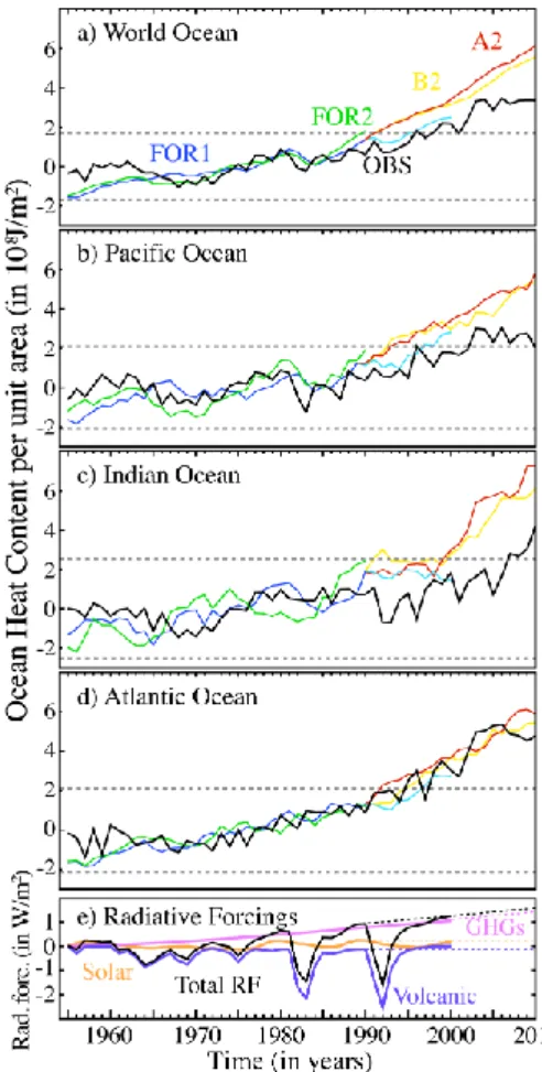
Fig. 2. (a–d) Evolution of OHC700 anomalies normalised per unit

area (in 108J m−2) in the upper 700 m of the world ocean and

the three main ocean basins. Observed OHC700 (OBS) is calcu-lated from temperature profiles of the Ocean Climate Laboratory at NODC. Simulated OHC700 anomalies are computed for the forced simulations FOR1 and FOR2 from 1955 to 1990, and for the sce-nario runs A2 and B2 from 1991 to 2010. A continuation to year 2000 AD in FOR1 is highlighted as a light blue line. Horizontal dashed lines represent a threshold of ±2 standard deviations from the long-term variability in CTRL. The reference period for the anomalies is 1960–1990. (e) Estimates of the radiative forcings ex-pressed as changes with respect to year 1955. Dotted lines corre-spond to projections of the radiative forcing in the A2 scenario run.

Our analysis will be therefore mainly focused on the long-term trends, and the representation of decadal OHC vari-ability. As for the observational records, the simulated OHC anomalies are computed in the upper 700 m of the ocean (hereafter referred as OHC700). Also, for a better compar-ison among the basins and the global ocean, the correspond-ing anomalies are calculated as heat content changes by unit area (Fig. 2). To cover the whole observational period (1955–2010) with the forced simulations, the first 20 yr of the future scenario runs A2 and B2 are shown after 1990. Note that OHC700 oscillates within the range of CTRL vari-ability (dashed horizontal lines in Fig. 2) from 1955 to 1990, and goes beyond these values afterwards. Since A2 and B2

(6)

A2 1955-1990 1991-2010 -2 -1.5 -1 -0.5 0 0.5 1 1.5 2 2.5 3 3.5 60E 120E 180 120W 60W 0 60E 120E 180 120W 30N 60N EQ 30S 60S 30N 60N EQ 30S 60S 30N 60N EQ 30S 60S 60W 0 OBS FOR1 A2 OBS 60E 120E 180 120W 60W 0 B2 FOR2 B2 2011-2100

Fig. 3. Linear trends of the observed (top panel) and simulated (lower panels) OHC700 (in 108J m−2yr) in the upper 700 of the ocean for the periods 1955–1990 (left), 1991–2010 (middle) and 2011–2100 (right).

assume zero volcanic activity and keep solar irradiance con-stant from year 1990 AD, they both miss the natural exter-nal influences. Note that the influence of Pinatubo’s erup-tion (in 1991 AD) is reproduced in the extended decade in FOR1 (light blue line). The corresponding variations in the different radiative forcings are also shown to allow a di-rect comparison with the OHC700 changes (Fig. 2e). Glob-ally, forced simulations are able to partly reproduce the low-frequency OHC700 modulation in observations associated with the cooling effect of volcanoes. Note that the remark-able OHC reduction in OBS coinciding with Mt Agung’s eruption in 1963 is not reproduced by either FOR1 or FOR2. This is possibly due to an underestimation in the simulations of the associated volcanic forcing, as two more recent esti-mates (i.e. Gao et al., 2008; Crowley et al., 2008) suggest a larger magnitude for this eruption, being actually of com-parable order to Pinatubo’s. These two new reconstructions have helped to highlight important uncertainties in volcanic activity concerning even the instrumental period (Schmidt et al., 2011). Also, both simulations and observations ev-idence that most decadal variability occurs in the Pacific and Indian oceans, while the Atlantic Ocean warms almost linearly. Discrepancies in decadal variability among FOR1, FOR2 and OBS (blue, green and black curves in Fig. 2) point to potential influences of natural climate variability in the Pacific and Indian basins, superimposed on the GHG-driven trend and the volcanic modulation. The global integral shows

better agreement since local effects are partly canceled out. Coefficients of determination (R2) between the OHC700 and the total radiative forcing are compared separately before and after 1990 (Table 1). The OHC700 variance explained by the forcing, both for the simulations and observations, is found to increase dramatically from below 30 % for 1955–1990 to about 70 % in the subsequent 20 yr. This large increase in the variance explained is mainly related to the steep warming trend after year 1990.

Regarding the trends (Table 2), all forced simulations over-estimate the global OHC700 trends, especially from 1955 to 1990, the period with largest observed decadal OHC700 vari-ability. This overestimation can be arguably attributed to the lack of sulphate aerosols in the forced simulations, which can partly offset the GHG warming up to 50 % (Delworth et al., 2005). By basins, trends are mostly overestimated in the Pacific (that dominates the warming due to its larger ex-tension) and Indian oceans, but show a good agreement in the Atlantic (Fig. 2b–d and Table 2), probably indicating that internal variability in this basin conceals the offset due to the missing contributions from changes in anthropogenic aerosols and the vegetation cover.

The spatial distribution of recent trends is now explored to identify robust features on the response to the forcing, and also local modulations by internal modes of variabil-ity. In the period 1955–1990 (Fig. 3, left column), agreement between observations and simulations is limited, suggesting

(7)

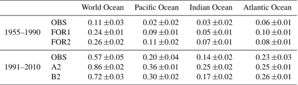
Table 1. Coefficients of determination R2between the OHC700 and the total equivalent radiative forcing during the periods 1955–2010,

1955–1990 and 1991–2010. In this particular case, the R2coefficient represents the fraction of OHC700 variance explained by the forcing,

and is calculated for the whole ocean and also individually for the three major basins. Values exceeding the 95 % confidence level according to a Student’s t test that takes into account the series autocorrelation to correct the sample size are highlighted in bold.

World Ocean Pacific Ocean Indian Ocean Atlantic Ocean

1955–2010 OBS 0.68 0.67 0.42 0.63 FOR1+A2 0.69 0.66 0.66 0.70 FOR1+B2 0.67 0.63 0.68 0.64 1955–1990 OBS 0.33 0.32 0.20 0.11 FOR1 0.13 0.04 0.22 0.14 FOR2 0.23 0.23 0.27 0.04 1991–2010 OBS 0.84 0.61 0.69 0.76 A2 0.99 0.98 0.90 0.97 B2 0.99 0.95 0.86 0.95

Table 2. Linear trends in OHC700 (in 1022J yr−1) during the periods 1955–1990 and 1991–2010 in the world ocean, and the three main basins. Uncertainties inherent to the least square regression method used to compute the trends are also provided.

World Ocean Pacific Ocean Indian Ocean Atlantic Ocean

1955–1990 OBS 0.11 ±0.03 0.02 ±0.02 0.03 ±0.02 0.06 ±0.01 FOR1 0.24 ±0.01 0.09 ±0.01 0.05 ±0.01 0.10 ±0.01 FOR2 0.26 ±0.02 0.11 ±0.02 0.07 ±0.01 0.08 ±0.01 1991–2010 OBS 0.57 ±0.05 0.20 ±0.04 0.14 ±0.02 0.23 ±0.03 A2 0.86 ±0.02 0.36 ±0.01 0.25 ±0.02 0.25 ±0.01 B2 0.72 ±0.03 0.30 ±0.02 0.17 ±0.02 0.26 ±0.01

an important role of internal variability. From 1991 to 2010 (Fig. 3, middle column), common features can be highlighted both in the observed and simulated trends, with larger ten-dencies in the North Atlantic and western Pacific, and a rather uniform warming in the Indian basin. Both simulations also show a patch of ocean heat loss to the north of the Ross Sea, which relates to a local decrease in convection over the re-gion that will be further discussed in Sect. 4.2. Note that ob-servations now show opposite trends with respect to those from 1955 to 1990 in both the Atlantic and Pacific oceans. This change in trends could be compatible with shifts in the phases of the PDO and the AMO indices among both periods. These contributions of natural variability will be further anal-ysed in Sect. 5. Other possible shifts in natural processes that can influence the observed OHC700 trends during the last 20 yr are the recent tendency to more negative NAO phases, a weakening of the SST gradients in the North Atlantic Cur-rent and the Irminger Basin (Flatau et al., 2003), and a de-cline in the strength of the North Atlantic subpolar gyre dur-ing the 1990s (H¨akkinen and Rhines, 2004) and of the At-lantic meridional overturning circulation (AMOC) in the last decade (Send et al., 2011). Finally, during the last 90 yr of the scenario runs (Fig. 3, right column) a worldwide warm-ing pattern emerges, with larger trends at high latitudes of the Northern Hemisphere. Yet a local OHC700 cooling south of

Greenland is also seen, in line with a local decrease in deep convection that reduces vertical heat mixing and thus the re-placement of dense cold waters at the surface with relatively lighter and warmer waters from deeper levels. This reduced convection is also compatible with the reported weakening of the AMOC cell in future scenario simulations (Schmittner et al., 2005).

Previous results suggest both a predominant influence of the forcing, most important from 1990, along with some im-pact of internal climate variability, able to produce important OHC700 changes at least at local scales. These results are however limited by the short time span of the observational period. The use of the millennial simulations will allow for a better understanding and quantification of these influences. In a first step, simulated OHC variability will be assessed for the last millennium.

3.2 Ocean heat content throughout the last millennium

The OHC variability throughout the last millennium is inves-tigated by assessing its simulated variations in the context of the total radiative forcing used as well as the proxy ev-idence available. Ocean heat content, when integrated over deep ocean levels, is a good indicator of decadal changes in the radiation balance at the top of the atmosphere (Palmer et al., 2011). However, due to the slow diffusion processes

(8)

-0.2 1000 2000 3000 4000 5000 1000 2000 3000 4000 5000 1000 2000 3000 4000 5000 1000 1200 1400 1600 1800 -0.2 -0.1 0 0.1 a) Temperature anomalies (in ºC) b) Trends in depth

1.6 1.4 1.2 1 0.8 0.6 0.4 0.2 0 -0.4 -0.6 -0.8 -1

Trend (in K/century) Time (in years)

CTRL

FOR1

FOR2

Fig. 4. (a) Hovmoller plot (depth vs. time) of the anomalous global

temperature (in ◦C) for CTRL, FOR1 and FOR2. The common

reference period is 1960–1990. (b) Long-term trends (green thick lines) of the ocean temperature means at different depths. In ad-dition, trends are also calculated in the first and second halves of CTRL (light blue and light green lines, respectively).

that govern its dynamics, the deep ocean requires several mil-lennia to reach steady conditions. The high computational cost of running fully coupled AOGCMs limits the length of simulations, which often precludes these from achieving a desirable equilibrium state at large depths. The resulting in-stabilities can partially mask the oceanic response to the ra-diative forcing, and even distort the regional imprints of in-ternal processes throughout the simulated period. Therefore, we start by analysing whether and to what extent these insta-bilities are present in the ECHO-G simulations considered herein.

All millennial ECHO-G simulations show important tem-perature trends at intermediate to bottom waters (Fig. 4). CTRL shows opposite long-lasting trends above and below 2000 m, with a strong initial imbalance (light blue line in top Fig. 4b) that gradually decreases (light green line in Fig. 4b) as the deep ocean slowly adjusts to current cli-mate conditions. Temperature trends are even more promi-nent at 1000 m depth in FOR1, where the ocean starts anoma-lously warm, clearly suggesting that the 100 yr spin-down period considered was insufficient to adapt the ocean state in CTRL to the forcing conditions in year 1000 AD. By contrast, FOR2, with starting conditions taken from year 1700 AD in FOR1 when the thermal imbalance was consid-erably reduced, shows smaller temperature trends, in

partic--200 0 200 200 SL Change (in mm) FOR1 FOR2 CTRL2 A2 B2 A2 B2

a) OHC700 and Sea Level Rise

b) Total effective radiative forcing

1000 1200 1400 1600 1800 2000 Time (years) 0 -5 5 10 15

OHC change (in 10 J)

23 Kemp11 Jev08 -8 -4 0 4 Total RF (in W/m ) 2

Fig. 5. (a) Anomalies of the simulated global OHC700 (in 1023J) and the reconstructed SL variations wrt the period 1960–1990. SL curves correspond to observations from tide gauges since 1700 AD (brown line; Jevrejeva et al., 2008) and to an idealized summary curve for the last millennium from proxy reconstructions with salt-marsh sediments in North Carolina; (b) Effective radiative forcing

applied to the forced simulations (in W m−2).

ular for the upper ocean. It is not clear, however, if the simu-lated trends in FOR2 can be entirely associated to the effect of radiative forcing, or if some remaining imbalance is still present.

Figure 5a illustrates the simulated OHC700 for the last millennium. FOR1 and FOR2 show comparable variability since 1700 AD, but prior to this year FOR1 appears to be clearly influenced by the warm starting conditions. Neither FOR2 nor CTRL show remarkable trends attributable to an initial thermal imbalance. However, both simulations have important instabilities when the complete ocean depth is con-sidered.

A comparison with proxy data is now established (Fig. 5a). Given the lack of direct paleo records of past OHC variabil-ity, estimates of SL variability are used instead. The longest instrumental SL record is computed from tide gauge obser-vations since 1700 AD (Jevrejeva et al., 2008). Caution is re-quired for its interpretation as a global estimate since only three gauges were included before 1860, and these are biased to Northern Europe (i.e. Amsterdam, Liverpool and Stock-holm). The record shows evidence that acceleration of sea level rise began about 200 yr ago, and was preceded by a cen-tury of comparatively flattened SL variations (brown line in Fig. 5a). A local reconstruction from salt-marsh sediments in North Carolina (Kemp et al., 2011), summarised in an idealised manner by the yellow filled curve in Fig. 5a, is in

(9)

FOR1 60E 120E 180 120W 60W 0 60E 120E 180 120W 60W 0 30N 60N EQ 30S 60S

OBSInstrumental Period (1955-2000)

15 12 9 6 0 -12 -9 -6 -3 -15 3

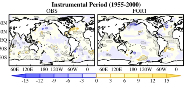
Fig. 6. Regression patterns between the OHC700 anomalies (in

108J m−2) and the standardised total radiative forcing in Fig. 2

during the period 1955–2000 of the observations and the extended FOR1 run. Dotted areas enclose values exceeding the 95 % confi-dence level according to a Student’s t test that takes into account the series autocorrelation to correct the sample size.

broad agreement with estimates in Jevrejeva et al. (2008), and shows stable SL variability during the same period. However, it should also be noted that the exact timing at which accel-eration of SLR starts in the reconstruction of Kemp11 can be sensitive to the method considered for subsidence adjustment (See Fig. 1 in Grinsted et al., 2011).

Given the large temperature trends in the deep ocean even in FOR2 (Fig. 4), which would introduce a drift in the simu-lated thermal expansion, and keeping in mind that none of the other contributions to sea level change, such as the melting of land glaciers or the polar ice caps, as represented in the ECHO-G model, SL estimates are directly compared with the simulated OHC700 (Fig. 5a). Despite the misrepresented processes, and the constraint to the upper 700 m, the simu-lated OHC and reconstructed SL changes show similar vari-ations from 1500 AD onwards. Note in particular the similar onset for the recent upper ocean warming and the observed SLR two centuries ago. The largest discrepancies occur dur-ing the first five centuries of the millennium, where none of the forced simulations follow the steady increase of SL in the reconstruction of Kemp11. However, in both simulations, and in particular in FOR2, there is a great degree of coher-ence between the curves of OHC700 and the total radiative forcing (Fig. 5a, b), as it will become evident in Fig. 9. This good agreement is incompatible with the initial trend in SL reconstructions and also suggests that the initial thermal im-balance in FOR2 has a negligible impact when integrated at this particular depth. Therefore, from now on, analyses cov-ering the last millennium will only be addressed with FOR2, and will be restricted to the upper 700 m of the ocean. FOR1, together with the scenario simulations, will be considered only for analyses centred on the observational period, when the thermal initial instabilities are mostly balanced, as sug-gested by the great accordance between both forced runs.

4 Fingerprint of external forcing on ocean heat content

OHC700 shows a good correspondence with variations in the net radiative forcing (Fig. 5a and b, respectively). The main aspects of this influence are now discussed.

4.1 Quantifying recent forcing impacts

The last 55 yr have witnessed relevant changes in the radia-tive forcing, mainly associated with an acceleration of both GHG and sulphate aerosols emission rates and the occur-rence of three major volcanic eruptions (Mt. Agung in 1963; El Chich´on in 1982 and Pinatubo in 1991) and five complete solar cycles. In response to these changes, the world ocean has experienced a remarkable warming trend, modulated to some extent at decadal timescales (Fig. 2). In this context, however, impact and attribution studies are constrained by the short time span of the observational records. Particular caution should be taken since physically unrelated quantities can coincidentally vary at comparable timescales. We now assess the relation between the external forcing and upper OHC both in the observations and the model. To ensure that no artificial relationship emerges in our regression analyses, a statistical significance test is employed that takes into ac-count the serial autocorrelation to correct for the effective sample size (Bretherton et al., 1999).

In order to maximise the signal of the oceanic response, the analysis in the observational period is exclusively fo-cused on the effect of the total radiative forcing. The period considered for the analysis is 1955–2000, to include the lat-est changes in solar and volcanic forcing used for the ex-tended FOR1 run. Figure 6 shows the regression patterns be-tween the total radiative forcing in this experiment (black line in lower panel of Fig. 2) and the observed and simu-lated OHC700 global fields. Coherence between both plots is limited and there is a general disagreement in the regions where the largest significant changes occur. This points to a probable different role of internal variability in this period for the two datasets. Also, this calculation can be affected by the absence of anthropogenic aerosols in the simulations, which may be crucial to explain recent decadal changes in North Atlantic climate (Booth et al., 2012). The validity of these results will be assessed in the next section by extend-ing the analysis to the whole FOR2 run. This will allow for providing further insight into the role of each forcing factor.

4.2 Influence of the forcing in the last thousand years

Within the last millennium, the pattern of response to an in-crease in the total radiative forcing (Fig. 7a) corresponds to a generalised warming of the upper ocean, with larger values in the extratropics, and some local coolings in regions of deep convection, like the Labrador and Ross Seas. In this latter re-gion both convection and the OHC700 respond differently to the radiative forcing than in the rest of the Southern Ocean

(10)

d) Ef. Solar Constant (with volcanoes) 60E 120E 180 120W 60W 0 30N 60N EQ 30S 60S 30N 60N EQ 30S 60S

a) Total Radiative Forcing b) Greenhouse Gases

c) Solar Irradiance

e) Top 10 preindustrial eruptions f) 15 intermediate preindustrial eruptions 30N 60N EQ 30S 60S 60E 120E 180 120W 60W 0 15 12 9 6 0 -12 -9 -6 -3 -15 3

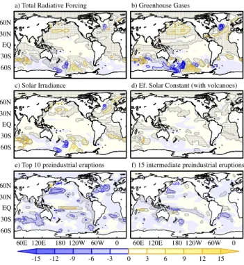
Fig. 7. (a–d) Regression patterns in FOR2 between the OHC700

anomalies (in 108J m−2) and the standardised series of the total

ra-diative forcing, the equivalent forcing of GHGs, the solar irradiance and the effective solar constant, i.e. solar irradiance+radiative ef-fect of volcanic aerosols, respectively. Significance is addressed as in Fig. 6. (e–f) Composite of the OHC700 differences between the 5 yr following and 5 yr preceding the top 10 and the next 15 largest preindustrial eruptions. Significance is established at the 0.05 level through a Monte Carlo test based on 1000 random selections in CTRL.

due to its particular stratification conditions. The Ross Sea is characterised by climatologically colder waters in the up-per 700 m than in the levels underneath (not shown), so that a corresponding decrease in convection will reduce vertical heat mixing between both layers, thus producing the local cooling in OHC700. By contrast, the rest of the Southern Ocean, and in particular the regions where convection is not important, will tend to warm following the increase in the radiative forcing.

Considering the individual effect of different factors, only the GHGs exhibit a widespread impact. In particular, they have a significant effect in the Tropics (Fig. 7b) and the con-vection regions, being also associated with the largest regres-sion coefficients. By contrast, the fingerprint of solar vari-ability (Fig. 7c) is characterised by a mild response mainly localised at midlatitudes in the three major basins. In either case, both forcings factors are the only ones to exhibit the lo-cal cooling in the Ross Sea, which might therefore require a gradual adjustment of convection to the changes in the radia-tive forcing. Part of the good agreement between the regres-sion patterns in Fig. 7b, c might rise from the fact that the

Fig. 8. In-phase regression patterns in FOR2 between the

standard-ised total radiative forcing and (a) the total cloud cover (in %), (b–f)

the different components of the net surface heat flux (in W m−2).

Note that positive heat flux values indicate that the flux goes into the ocean. Significance is addressed as in Fig. 6.

respective time series for the solar activity and the GHG con-centrations are not independent, since both undergo a gradual increase during the industrial period (Supplement Tables 1 and 2). Indeed, when the long-term frequencies are filtered out, the regression coefficients for the solar irradiance be-come insignificant in regions like the tropical Atlantic and the Labrador Sea (Supplement Fig. 1), thus indicating that these are actually related to the GHG curve. Note also that during the preindustrial period the global influence of GHGs is substantially reduced, and solar irradiance only shows sig-nificant impacts on the southern extratropics and the Nordic seas (Supplement Fig. 2). Regression values with the effec-tive solar constant (i.e. solar irradiance plus the radiaeffec-tive ef-fect of volcanoes) are considerably lower (Fig. 7d), as it is also punctuated by the episodic influence of volcanic erup-tions, which is clearly not linear. The impact of volcanoes is thus evaluated through a composite analysis focused sep-arately on the top 10 and the subsequent 15 largest prein-dustrial eruptions to distinguish the strong from the moder-ate impacts. Composite maps are calculmoder-ated by averaging the differences in OHC700 occurring between the 5 yr follow-ing and the 5 yr precedfollow-ing the selected volcanic eruptions, and their significance is assessed by comparing with the 2.5

(11)

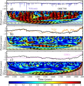
Total R F Time (years) 0 -5 5 P er io d (y ea rs ) 4 8 16 32 64 128 256 OHC700 1000 1100 1200 1300 1400 1500 1600 1700 1800 1900 2000 0 0.1 0.2 0.3 0.4 0.5 0.6 0.7 0.8 0.9 1

Fig. 9. Top: standardised time series of the total radiative forcing

and the OHC700 changes in the FOR2 simulation. Bottom: squared wavelet coherence between both time series. The black contours en-close areas where the coherence is significant at a 5 % level accord-ing to a Monte Carlo test. The arrows indicate the phase of their in-terrelationship (eastward arrows account for phase zero). Note that positive phases (represented by northward arrows) correspond to the forcing leading the OHC700 changes. The cone of influence (thick black curve) accounts for the region the edge effects become impor-tant.

and 97.5 percentiles of a Monte Carlo ensemble consisting of 1000 analogous differences in CTRL. As for the solar irradi-ance, the largest OHC700 changes take place in the extra-tropics (Fig. 7e–f). The pattern of cooling is similar in both composite analyses, with no remarkable spatial differences. As expected, larger negative anomalies are observed for the strongest eruptions (Fig. 7e). Also of note is the warming in the central equatorial Pacific for the strong volcanoes, thus in line with an influence of explosive volcanism on the occur-rence of El Ni˜no events (Emile-Geay et al., 2008).

The reasons for both the different latitudinal OHC700 re-sponse to the forcing and the larger sensitivity in the extra-tropics are now explored. Net heat into the ocean will result from the integration of all heat fluxes at the surface, and these can be controlled by changes in cloud coverage. Regression patterns in Fig. 8 illustrate how these variables are affected by the total radiative forcing. Interestingly, a general decrease in extratropic cloud coverage (Fig. 8a) follows the positive changes in the RF. This same pattern, but with opposite sign, characterises the changes in shortwave radiation (Fig. 8b), as it responds inversely to variations in cloud albedo, thus ex-plaining the larger OHC700 values at midlatitudes in Fig. 7. Other important features to note are a remarkable increase of cloud coverage over the Ross Sea and the convection re-gions of the North Atlantic, which reduce the shortwave in-coming radiation at the surface. In the Southern Ocean these latter changes are counterbalanced by opposite contributions of the other heat flux components (Fig. 8c–e). Also of note is a weak but widespread surface warming related to changes in long-wave radiation (Fig. 8c), and a notable ocean heating across the Gulf Stream and subpolar gyre responding to both latent and sensible heat flux changes (Fig. 8b, c).

Volcanic Solar GHGs Time (years) 1000 1100 1200 1300 1400 1500 1600 1700 1800 1900 2000 −10−5 0 OHC700 4 8 16 32 64 128 256 −20 2 4 8 16 32 64 128 256 −2 2 4 0 4 8 16 32 64 128 256 Period (years) Period (years) Period (years) a) b) c) 0 0.1 0.2 0.3 0.4 0.5 0.6 0.7 0.8 0.9 1

Fig. 10. The same as in Fig. 9 but for OHC700 and the standardised

series of (a) volcanic forcing, (b) solar irradiance, and (c) effective GHG forcing.

Adding up all the different influences (Fig. 8f), there is a worldwide net surface warming following the increases of the RF, with larger values in the regions of ocean deep con-vection of the Labrador and Ross Seas and also in the extrat-ropics. In both deep water formation regions the radiatively-forced surface warming reduces convection activity through its effect on ocean stratification. As a result, the upper ocean experiences a net cooling, as was observed in Fig. 7a. In the rest of the ocean the warming is observed both at the surface and integrated in depth, the OHC700 increase being there-fore related to the downward penetration of the net positive heat flux into the ocean. Note that this larger response at mid-latitudes is partly linked to a local increase of solar radiation at the surface following a significant reduction in cloud cov-erage. This particular pattern is not observed for the other surface heat fluxes.

We now turn our attention to the temporal features as-sociated with the influence of the different radiative forc-ings. A wavelet coherence (WTC) analysis (Torrence and Compo, 1998) is used to investigate the common spec-tral features between the OHC700 and the different forc-ings throughout the last millennium (Figs. 9 and 10). For all practical purposes, wavelet coherence can be regarded as a localised correlation coefficient but in time frequency space. All plots are generated with the software package pro-vided in Grinsted et al. (2004), following their recommen-dations for the choice of the wavelet transform (i.e. Mor-let function) and scale resolution (i.e. 10 scales per octave).

(12)

Likewise, significance is assessed using a Monte Carlo ap-proach based on an ensemble of 1000 surrogate dataset pairs with the same AR1 coefficients as the input time series. Note that wavelet coherence should be used and interpreted with caution. It is mostly an exploratory technique to test proposed linking mechanisms with a physical basis. Herein, WTC is used to explore the potential frequencies at which the forc-ing may have an impact on the OHC. Yet no definitive infer-ences on causality can be drawn. To help in the identification of robust linkages throughout time, phase-relationship is also computed at each time and frequency. The angle between the arrow and the x-axis indicates the phase between the forcing and OHC700. Thus, in-phase relationships are represented by eastward arrows in the wavelet coherence plots. At a par-ticular frequency band, whenever phase remains stable the physical link proposed will remain plausible.

The total equivalent radiative forcing shows a high de-gree of coherence with OHC700 variability at all timescales (Fig. 9), with changes in the forcing always leading (since arrows tend to have a small northward component) the heat content variations. In the preindustrial period, most of the co-herence comes from volcanoes, as highlighted by the good agreement between Figs. 9 and 10a. Note that coherence at interannual timescales is only present when the radiative forcing is punctuated by the effect of volcanism, as varia-tions in solar irradiance and GHGs occur at longer scales. Moreover, the influence of volcanic aerosols is also rele-vant at lower frequencies. Strong volcanoes impact as a step down signal on the OHC700 curve (Fig. 10a, upper panel), as it has been already described in other forced simula-tions (Gleckler et al., 2006; Gregory et al., 2006; Gregory, 2010). This signal, integrated during periods of intense vol-canism (e.g. 1150 to 1300 AD or 1550 to 1700 AD), can im-pact the OHC700 variability at multidecadal and even sec-ular timescales. Likewise, solar variability (Fig. 10b) shows some intervals of common variance with the OHC700 at in-terdecadal timescales. Finally, regarding the slowly-varying GHGs, high coherence arises at secular timescales during the last few centuries of the millennium, and at higher frequen-cies after the onset of the industrial era (Fig. 10c).

So far, the analysis has been centred on the instantaneous OHC700 response to the external forcing factors. Correla-tions in Fig. 11 illustrate their influence at other lags. For the total radiative forcing, significant correlations are found for lead times from 50 to 0 yr, and maximum values when it leads the OHC700 changes by 1–2 yr. This maximum impact is associated with the short-lived influence of volcanoes (blue line). By contrast, the slowly varying solar and GHG forc-ings show maximum correlations for lead times of 20 and 70 yr, respectively. This delayed response points to a grad-ual accumulation of the energy going into the ocean, the lag timescale being set by the cumulative effect of two consec-utive 11 yr cycles and the increasing GHGs, respectively. In-deed, a similar analysis for the period 1000–1700, when

nei--0.5 0 0.5 -100 -75 -50 -25 0 25 50 75 100 Correlation values Lag (years) OHC leads OHC lags Volcanic Solar GHGs Total RF

Fig. 11. Time-lag correlations in the whole FOR2 simulation

be-tween the OHC700 changes and the different radiative forcings. The thin coloured horizontal lines represent the threshold value for sig-nificance associated with each forcing. Dotted thin lines correspond to similar correlations but calculated for the period 1000–1700 (with no 11 yr solar cycle represented). Significance is assessed as in Fig. 6.

ther anthropogenic GHGs nor 11 yr solar cycles are included, shows leading times closer to zero (dotted lines in Fig. 11).

It has been shown that at higher frequencies, and in partic-ular at interannual timescales, coherence with the radiative forcing is limited (Fig 9) and only the volcanic forcing can explain some OHC700 variability. Hence, this is the range of frequencies at which internal variability is bound to account for a larger fraction of OHC700 variability.

5 OHC imprints of internal climate variability

5.1 Influence of internal variability over the last 55 yr

Previous sections suggest a potential role of internal modes of variability to locally modulate the upper ocean warming trends in the observational period. Globally, the impact of in-ternal climate variability on OHC700 appears to be largest at interannual to decadal timescales, especially during periods of low volcanic activity, when the effect of the radiative forc-ing is mainly observed at lower frequencies (interdecadal to secular; see Fig. 9). Other works (Willis et al., 2004; Levitus et al., 2005) also support the influence of different modes of climate variability on the OHC700. For example, there is par-ticular evidence that ENSO-related variability has produced noticeable interannual OHC700 changes during the obser-vational period (Willis et al., 2004). Thereby, other climate modes involving large-scale SST changes, such as the AMO or the PDO, can also potentially affect, locally or globally, the OHC700 budget. It is also known that predominant at-mospheric patterns, such as the NAO, can locally alter the air–sea heat fluxes at the ocean surface and trigger deep

(13)

convection events (Pickart et al., 2003), thus also contribut-ing to heat exchange with the deeper ocean.

A first evaluation of the influence of modes of climate vari-ability on the observed and simulated OHC700 is performed in the whole instrumental period (e.g. 1955–2010). For this analysis, the NAO and three well-known modes of SST vari-ability are explored, namely, ENSO (represented by El Ni˜no 3.4 index), PDO and AMO. In the forced simulations, the climate indices are calculated following similar definitions as for the observations. ENSO corresponds to El Ni˜no 3.4 index, defined as the mean SST value from 5◦S to 5◦N and 170–120◦W (Trenberth, 1997). The PDO index is derived as the leading PC of monthly SST anomalies in the North Pa-cific Ocean, poleward of 20◦N (Mantua et al., 1997). Like-wise, the AMO is defined as the regional average of Atlantic SST anomalies north of the Equator. Unlike in the AMO definition in Enfield et al. (2001), no previous detrending is applied to the SST data. Instead, to only preserve the sig-nal of intersig-nal natural variability unrelated to the forcing, all the three previous indices are computed with SST anomalies calculated with respect to the global SST mean, thus filter-ing out the influence of the global warmfilter-ing signal (Zhang et al., 1997). Indeed, in this way the three indices remain uncorrelated with the total radiative forcing (Supplement Ta-ble 3). Finally, the NAO is calculated as the leading mode of SLP anomalies in the North Atlantic (Wallace and Gutzler, 1981). It is worth mentioning that ENSO and NAO variabil-ity have been already evaluated in another control simulation with the ECHO-G model (Min et al., 2005b) through a com-parison with observations and other simulations. The overall model’s performance is good, although it presents some sys-tematic errors like an overestimation of the NAO impact over the Pacific sector, and stronger than observed ENSO ampli-tudes, which tends to be also too frequent and regular. Re-garding ENSO, the model resolves properly the Walker cir-culation, the associated rainfall over the tropical Pacific, and the anomalous warming from the central Pacific to the coast of South America. Likewise, the simulated NAO reproduces well the dipolar SLP structure over the North Atlantic, as well as the corresponding quadrupole in surface temperature, and the opposed precipitation pattern over the north and the south of Europe.

The impact of all indices on global OHC700 is assessed at two different frequency ranges: periods above and peri-ods below 5 yr (Table 3). At the higher frequencies, which mostly account for interannual events, only ENSO has a sig-nificant impact on OHC700, with R2 values close to 0.15 both in OBS and FOR1 + A2, and slightly lower in the whole FOR2 simulation. This finding is in line with Willis et al. (2004) who identified the signal of intense ENSO events in the global OHC integral. At the lowest frequencies, ob-servations show some covariability between the AMO and the total OHC700 (R2=0.20), although the R2coefficient is not significant when the sample size is corrected to take into account the time series autocorrelation. In the

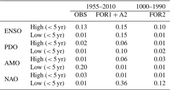
simula-Table 3. Coefficients of determination R2 between the global OHC700 and a selection of climate indices filtered separately at high (< 5 yr) and low (> 5 yr) frequency. Significance is assessed as in Table 1.

1955–2010 1000–1990 OBS FOR1 + A2 FOR2 ENSO High (< 5 yr) 0.13 0.15 0.10 Low (< 5 yr) 0.01 0.15 0.01 PDO High (< 5 yr) 0.02 0.06 0.01 Low (< 5 yr) 0.01 0.10 0.02 AMO High (< 5 yr) 0.01 0.06 0.03 Low (< 5 yr) 0.20 0.01 0.01 NAO High (< 5 yr) 0.03 0.01 0.01 Low (< 5 yr) 0.01 0.36 0.12

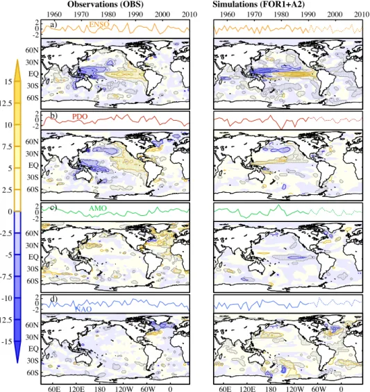
tions, only the NAO explains some meaningful part of the global OHC700 at low frequencies, although it could be just a consequence of a delayed NAO response to the forcing, which will be discussed later. To further compare the influ-ence of each index in the simulations and observations, their corresponding regional OHC700 fingerprints are illustrated in the regression patterns of Fig. 12. The observed ENSO and PDO indices exhibit similar patterns, with the former showing stronger equatorial anomalies and the latter showing larger impact in the North Pacific. Generally, both patterns are associated with an eastern warming and a western cool-ing of the upper Pacific Ocean. This result is consistent with the hypothesis that the local shift in OHC700 trends from 1955–1990 to 1991–2010 (see Fig. 3) is due to a change in the polarity of the PDO at the end of the 1970s. By contrast, in the model the zonal dipole structure is only observed at the Equator for the ENSO index, and at the North Pacific for the PDO, suggesting that the model cannot capture the coupling between both modes (Newman et al., 2003). Some aspects of the ENSO teleconnection with surface temperature in the Southern Ocean (e.g. Liu et al., 2004) can be identified in the observations, but not in the simulations. In particular, ob-servations show a significant warming north of the Amund-sen Sea, with opposing changes in the BellingshauAmund-sen and Weddell Seas, although these latter remain insignificant. Re-garding the AMO, it relates in the observations to positive OHC700 anomalies over the whole Atlantic, but shows no significant changes in FOR1 + A2. This probably indicates that, given the limited time period, no relevant changes of this index are taking place in the simulations. Finally, the most significant impact of the NAO is a cooling over the Labrador and Irminger Seas in the observations, partly repro-duced in the simulations. This cooling is likely responding to changes in convection, which is also affected by the NAO over both regions (Dickson et al., 1996; Pickart et al., 2003). Besides, an OHC700 increase is simulated at midlatitudes, similar to the one already described in response to the radia-tive forcing (Fig. 7). Therefore, this imprint is more probably

(14)

2 -20 2 -20 2 -20 ENSO PDO AMO NAO 2010 a) 15 12.5 10 7.5 5 0 -12.5 -10 -2.5 -5 -7.5 -15 2.5 30N 60N EQ 30S 60S

Observations (OBS) Simulations (FOR1+A2)

b) 30N 60N EQ 30S 60S 30N 60N EQ 30S 60S d) 30N 60N EQ 30S 60S 60E 120E 180 120W 60W 0 1990 1980 1970 1960 2000 c) 2 -20 2010 1990 1980 1970 1960 2000 60E 120E 180 120W 60W 0

Fig. 12. Top: observed (left) and simulated (right) standardised indices of: (a) El Ni˜no 3.4; (b) PDO; (c) AMO; (d) NAO. See text for details

on the particular definitions applied. Dashed lines correspond to projections in the A2 scenario run. Bottom: regression patterns between the

anomalies of OHC700 (in 108J m−2) and the indices above. Significance is addressed as in Fig. 6.

associated with the recent changes in the forcing, which may be also having an impact on NAO variability. Indeed, the fi-nal tendency to negative NAO values in the observations can explain the remarkable warming of the North Atlantic since year 1990 (see Fig. 3). In the next subsection, the analysis is extended to the last thousand years, to better determine the spatial impacts associated with the previous modes and the predominant timescales of their influence.

5.2 Modes of climate variability and OHC in the last millennium

The regression patterns in Fig. 12 are now calculated for the complete FOR2 simulation (Fig. 13). The patterns cor-responding to ENSO and the PDO are similar to those de-scribed during the observational period. The AMO is now related to a general warming in the North Atlantic, more in line with the OHC700 pattern described for the observations.

It also shows a local cooling in the Labrador Sea and some positive OHC700 anomalies in the North Pacific, near the region where the PDO occurs. Similar features are also ob-served in the pattern of the NAO (Fig. 13d). This suggests a link between the three modes in the model. Indeed, the AMO is known to be related to changes in the AMOC (Knight et al., 2005), the latter being driven by changes in the NAO in the forced simulations (Ortega et al., 2012). Also, the interrela-tionship between the NAO and the Arctic Oscillation (AO) may explain an atmospheric influence over the North Pacific, and thereby on the PDO. The lead-lag relationship at low-frequencies between the previous indices in the model is ex-plored in Fig. 14 for the whole FOR2 simulation. The NAO leads the AMO and PDO changes by 2 and 4 yr, respectively. Furthermore, the radiative forcing is found to have a leading role on the NAO, which lags the total RF changes by about 1 yr.

(15)

15 10 12.5 7.5 0 -10 -7.5 -5 -2.5 2.5 -15 -12.5 5 30N 60N EQ 30S 60S a) ENSO c) AMO d) NAO b) PDO 30N 60N EQ 30S 60S

60E 120E 180 120W 60W 0 60E 120E 180 120W 60W 0

I

II

III

IV

Fig. 13. Regression patterns between the OHC700 anomalies (in

108J m−2) and the following standardised climate indices in the

whole FOR2 simulation: (a) El Ni˜no 3.4; (b) PDO; (c) AMO; (d) NAO. Significance is addressed as in Fig. 6. The black dotted rect-angles delimit the regions assessed in the wavelet coherence analy-sis of Fig. 15. Boxes are defined for each climate index to average the OHC700 anomalies over the regions where their fingerprint is larger.

The influence of these modes in the OHC700 variations is now explored in a temporal and spectral perspective. For this, a wavelet coherence analysis is again employed (Fig. 15). In the previous analysis of the forcings, which have a worldwide impact on the OHC700, the coherence was established with respect to the global OHC700 integral. In this case, how-ever, the different modes produce more localised influences, and thereby coherence is investigated regionally. Each index is compared with the OHC700 average in the region where its influence is originally taking place (dotted rectangles in Fig. 13). Note that OHC700 variability in these four regions (dark curves in top panels of Fig. 15) still presents a mod-ulation by the external forcing at the very lowest frequen-cies (beyond centennial). Yet they also exhibit other predom-inant scales of variability at higher frequencies, which are potentially attributable to the local modes. For ENSO, both time series (i.e. El Ni˜no 3.4 and the OHC700 average in the equatorial Pacific) show a high degree of coherence at inter-annual timescales, and also relatively good agreement from decadal to multidecadal timescales. Although in some par-ticular periods (e.g. 1100–1300) coherence is damped above decadal timescales, overall ENSO explains most of OHC700 variability over the equatorial Pacific. Regarding the PDO and AMO, both indices show alternating periods of good and poor coherence with the local OHC700 at multidecadal timescales. The fact that the phase of the relationships (ar-rows in Fig. 15) remains stable throughout the whole sim-ulation, with westward arrows in Fig. 15b accounting for a North Pacific cooling and eastward arrows in Fig. 15c

rep--0.5 0 0.5 -15 -10 -5 0 5 10 15 Correlation values Lag (years) NAO leads NAO lags Total RF _AMO PDO

Fig. 14. Time-lag correlations between the decadally low-pass

fil-tered indices of the NAO and the following time series: the PDO (red line), the AMO (green line), and the total radiative forcing (black line). Correlations are calculated for the complete FOR2 sim-ulation. The thin coloured horizontal lines represent the threshold value for significance associated with each series. Significance is addressed as in Fig. 6.

resenting a mid-latitude North Atlantic warming, both com-patible with the corresponding OHC700 patterns in Fig. 13, suggests that the OHC may be responding during those time periods to the particular phases of the PDO and the AMO. The reasons for this discontinuous influence are not clear to us, although some impact of the radiative forcing cannot be excluded. Indeed, Fig. 7 showed that OHC700 in both re-gions, unlike in the equatorial latitudes, is particularly sen-sitive to changes in the radiative forcings. There is also the possibility that other modes of variability are masking part of the signal. Finally, the NAO shows a good degree of coher-ence with interannual and interdecadal OHC700 variability in the Labrador Sea, although subject again to some periods of intermittence. Interestingly, the phase of this relationship changes at different timescales. For periods up to 30 yr, the westward arrows indicate a direct association between the NAO and a cooling over the Labrador Sea, as expected given the leading role of the NAO on both North Atlantic convec-tion and the AMOC discussed in OR12. At longer timescales some periods (e.g. 1300–1500) give evidence of the opposite relationship. As the NAO has been found to respond to vari-ations in the total radiative forcing (Fig. 14), the Labrador warming observed at low frequencies could be actually at-tributed to a direct OHC700 response to this forcing.

6 Conclusions and discussion

The upper OHC response to the external forcing as well as the fingerprint of several modes of climate variability have been assessed in a suite of observations and model simula-tions covering the period 1000 to 2100 AD.

(16)

ENSO PDO AMO NAO a) b) c) OHC box-I Period (years) −20 2 OHC box-II 4 8 16 32 64 128 256 4 8 16 32 64 128 256 Period (years) −2 −4 0 2 4 OHC box-III Period (years) −20 2 OHC box-IV Period (years) −20 2 d) 1000 1100 1200 1300 1400 1500 1600 1700 1800 1900 2000 Time (years) 4 8 16 32 64 128 256 4 8 16 32 64 128 256 0 0.1 0.2 0.3 0.4 0.5 0.6 0.7 0.8 0.9 1

Fig. 15. The same as in Fig. 9 but between the standardised indices

of ENSO, PDO, AMO and NAO and the OHC700 averages in the corresponding boxes defined in Fig. 13. In the top panels time se-ries are smoothed with a 10 yr low-pass filter to ease comparison at interdecadal timescales.

In the instrumental period, the model overestimates the warming trend and underestimates the decadal OHC700 vari-ability. The misrepresentation in trends is explained to some extent by the lack of sulphate aerosols in the simulations, whose cooling effect is known to partially offset the GHG-driven warming (Delworth et al., 2005). Note that aerosols have also been proposed to be a main contributor to North Atlantic decadal variability over the last century (Booth et al., 2012). The spatial distribution and intensity of the up-per OHC warming trends have changed from 1955–1990 to 1991–2010. These changes respond, respectively, to a sus-tained increase of the net radiative forcing (mostly associ-ated with an acceleration of GHG emissions) and a shift in the values of the PDO and AMO indices.

All the long simulations are found to exhibit initial ther-mal instabilities, which in the case of FOR1 and FOR2 obey too short a spin-down period to bring the ocean to thermal equilibrium with the forcing conditions in year 1000 AD. To minimise the effect of the corresponding drift in temperature, the analysis only focuses on the OHC in the upper 700 m, where the CTRL run remains stable and FOR2 shows a good correspondence both with the net radiative forcing and two paleo records of global sea level change.

The spatial imprint of the radiative forcing has also been analysed. All the individual forcings show a similar impact, with larger effect at extratropical latitudes. This larger re-sponse at midlatitudes is partly explained by a local

reduc-tion in cloud cover, thus allowing a larger fracreduc-tion of solar radiation to reach the ocean surface. Other contributions to the net surface heat flux, such as the outgoing longwave ra-diation or the sensible and latent heat fluxes, do not repro-duce this different latitudinal response. In the preindustrial era, a large part of the forced OHC700 variability is associ-ated with volcanism, with some solar contribution at inter-decadal timescales (periods from 10 to 100 yr). After 1850, low-frequency OHC700 variability is mainly responding to the increased GHG concentrations, and the influence of vol-canic activity remains important at decadal and intradecadal timescales. Interestingly, the ocean shows a delayed response to all the radiative forcings, with the largest impacts occur-ring about 2, 20 and 70 yr after the changes in volcanic, solar and GHG forcing, respectively.

Finally, the contributions from four large-scale modes of climate variability have been explored (i.e. ENSO, the PDO, the AMO and the NAO). As their influence on the OHC700 is larger at regional scales, their spectral features have been directly analysed in their respective centres of action. In these four regions the long-term OHC700 variations still ex-hibit some modulation by the external forcing. Yet at shorter timescales (annual to secular) the regions show periods of spectral coherence with their corresponding climate indices. The influence of ENSO is mainly localised in the equatorial Pacific, where it is found to dominate the local OHC700 vari-ability from interannual to multidecadal timescales. Like-wise, positive PDO and AMO indices relate, respectively, to a cooling in the North Pacific and warming at midlati-tudes in the North Atlantic, both modes contributing discon-tinuously to OHC700 variability at multidecadal timescales. The NAO, in the model and observations, produces a cooling over the Labrador Sea, which in the simulations gives rise to a strengthening of the AMOC cell. This impact takes place from interannual to interdecadal timescales. Furthermore, the fact that natural modes of climate variability, such as ENSO, NAO or AMO, can impact the OHC700 globally or locally is important for the coming decades, since they can temporarily mitigate or intensify the ocean warming signal and they can modulate as well the regional sea level rise.

To assess the general relevance of these results, we now discuss the limitations of the ECHO-G model, and put it in the context of other AOGCMs. The major constraint relies on the use of flux adjustments (and more in particular heat flux corrections), since they can largely affect the ocean heat con-tent and its regional patterns. However, a comparison of these terms with the actual fluxes at the surface (see Supplement Table 4 and Fig. 3) shows that in overall, and in particular in the centres of action of ENSO, the AMO and the NAO, the magnitude of heat adjustments remains considerably smaller, thus suggesting that their probable impact on ocean heat up-take is also small (Sausen et al., 1988). In contrast, freshwa-ter adjustments remain comparably important, particularly across the Gulf Sream, thus evidencing that some ocean dy-namics are misrepresented by the model, and thereby casting