Adaptive Thermal Modeling Architecture For Small Satellite
Applications
by
John Anger Richmond
B.S., United States Air Force Academy (2008)
Submitted to the Department of Aeronautics and Astronautics
in partial fulfillment of the requirements for the degree of
Master of Science in Aeronautics and Astronautics
at the
MASSACHUSETTS INSTITUTE OF TECHNOLOGY
June 2010
@
Massachusetts Institute of Technology 2010. All rights reserved.
ARCHNES
MASSACHUSETS INSTf UTE.OF TECHNOLOGY
JUN 2 3 2010
LIBRARIES
A uthor ...
Department of Aeronautics and Astronautics
May 11, 2010
Certified by...
Certified
by...
Accepted by ...
Colonel John Keesee, USAF Retired
Senior Lecturer
Thesis Supervisor
. . . .
. . . ..
David W. Miller
Professor of Aeronautics and Astronautics
Thesis Supervisor
/IJ
Eytan H. Modiano
Associate(Professor of Aeronautics and Astronautics
Chair, Committee on Graduate Students
Adaptive Thermal Modeling Architecture For Small Satellite
Applications
by
John Anger Richmond
Submitted to the Department of Aeronautics and Astronautics on May 11, 2010, in partial fulfillment of the
requirements for the degree of
Master of Science in Aeronautics and Astronautics
Abstract
The United States Air Force and commercial aerospace industry recognize the importance of moving towards smaller, better, and cheaper spacecraft to support the nation's increasing dependence on space-based technologies. Whether large or small, all spacecraft will require the same basic bus systems and environmental protection, simply scaled to fit the mission. The varying thermal environment in space is particularly important to spacecraft design and operation because of its affect on hardware performance and survivability. The Adaptive Thermal Modeling Architecture (ATMA) discussed in this thesis is meant to bridge the gap between the commercially available thermal modeling tools used for larger, more expensive satellites, and the low-fidelity algorithms and techniques used for simple first order analysis. The ATMA consists of the MATLAB based Adaptive Thermal Modeling Tool (ATMT) and its user's manual, as well as the process by which an inexperienced engineer can quickly and accurately perform on-orbit thermal trades studies for a range of space applications. The ATMA tools and techniques have been validated with an industry standard thermal modeling program (Thermal Desktop) and correlated to thermal test data taken from MIT's CASTOR nanosatellite. The concepts derived and evaluated within ATMA can be extended to a variety of aerospace modeling applications. The ATMT program and modeling architec-ture are currently being utilized by members of MIT's Space Engineering Academy (SEA) and undergraduate satellite team as well as the U.S. Air Force Academy's FalconSAT-6 program.
DISCLAIMER CLAUSE: The views expressed in this article are those of the author and do not reflect the official policy or position of the United States Air Force, Department of Defense, or the U.S. Government
Thesis Supervisor: Colonel John Keesee, USAF Retired Title: Senior Lecturer
Thesis Supervisor: David W. Miller
Acknowledgments
I would first like to thank my parents Robert and Carol Richmond for their love and support throughout my entire life. Their confidence and faith in me provided the inspiration I needed to make it through the numerous obstacles I have encountered throughout my life.
Special thanks goes to my two advisers Colonel John Keesee, USAF retired and Professor David W. Miller for mentoring me throughout my two years at MIT. Colonel Keesee has always helped me to see the bigger picture and kept me focused on the light at the end of the tunnel. Additionally, he has helped with both the technical and narrative content within my thesis. As both an engineer and an officer in the U.S. Air Force, Colonel Keesee has been an excellent role model and personal mentor. Professor Miller is gave me the opportunity to attend MIT and be a part of something innovative and exciting. He was always there to evaluate and question my technical research challenging me to go beyond my field of expertise and discover new methods for problem solving.
I am indebted to the U.S. Air Force and my mentors at the U.S. Air Force Academy.
The Air Force has given me the opportunity to defend my country and afforded me the education and tools to so effectively. My Air Force mentors prepared me physically and mentally for MIT and without their trust and confidence I could never have made it this far. I aspire to live up to the precedent they have set for me and to accomplish the successes that they have helped me to envision.
I would like to recognize senior Chris Flatley of the University of Colorado Colorado Springs, for supporting my research by developing and testing the correlation models used to validate my Adaptive Thermal Modeling Tool (ATMT).
Of course, I could not have succeeded without my friends. Friends from the Space
Systems Lab at MIT; Joe Robinson, George Sondecker, Corey Crowell, and Matthew Mc-Cormack, who endured the same pains and grief and always offered a helping hand. Friends from my adolescence who always provided a warm welcome home and an escape from the bitter winters in Boston.
Contents
1 Introduction 19
1.1 Problem Statement . . . . 21
1.2 Thesis Motivation .... . . . . . . . . 21
1.3 Thermal Modeling Options . . . . 22
1.4 Research Gap Analysis. . . . . 26
1.5 Thesis Overview . . . . 30
2 Background 33 2.1 Spacecraft Size Hierarchy . . . . 34
2.2 Small and Nanosat Thermal Control Systems . . . . 37
2.2.1 Thermal Margin . . . . 37
2.3 Keplerian Orbit . . . . 39
2.3.1 Spacecraft Position and Velocity . . . . 41
2.3.2 Spacecraft Attitude On-orbit . . . . 42
2.4 Heat Transfer in the Space Thermal Environment . . . . 43
2.5 Conduction . . . . 44
2.6 Radiation . . . . 45
2.6.1 External Radiation . . . . 46
2.6.2 Internal Radiation.. . . . . . . . 49
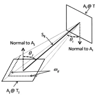
2.6.3 Radiation View Factors . . . . 50
2.7 Material Properties . . . . 52
2.7.1 Thermal Properties . . . . 52
3 Adaptive Thermal Modeling Architecture (ATMA)
3.1 Prediction Model (ATMT) ...
3.1.1 View Factor Algorithm ...
3.1.2 Ray Polygon Intersection Algorithm ...
3.1.3 View Factor from a Surface to Earth ...
3.1.4 Conductance Algorithm . . . .
3.2 Thermal Model Validation Techniques . . . . 3.2.1 Component Level Testing . . . .
3.2.2 CASTOR Thermal Vacuum Test . . . .
3.2.3 Sum m ary . . . .
4 Adaptive Thermal Modeling Tool
4.1 Modeling Assumptions . . . . ..
4.2 Thermal Model Inputs . . . .
4.3 Thermal Model Outputs . . . . .
4.4 Model Functionality . . . .
4.4.1 Test Case Overview . . .
4.5 ATMT Validation. . . . . ..
4.5.1 Validation of Test Case 1:
4.5.2 Validation of Test Case 2:
4.5.3 Validation of Test Case 3:
4.5.4 Validation of Test Case 4:
4.6 Model Performance . . . . 4.6.1 ATMT Accuracy . . . . . 4.6.2 ATMT Usability . . . . . (ATMT) 2D 3D 2D 3D Surac... Surface . . . . Solid Rectangle . Six Surface Box
Six Panel Box with Avionics Stack
5 ATMT User's Manual
5.1 Overview . . . .
5.2 ATMT Home Tab . . . 5.3 Geometry Tab . . . . .
5.4 View Factors Tab . . . .
5.5 Conductance Tab . . . . 5.6 Material Properties Tab
129 . . . . . . . . 1 3 0 . . . . 1 3 1 . . . . 13 2 . . . . 14 3 . . . . . . . . . . . . 14 6 . . . . . . . 1 5 0 57 58 59 66 69 71 74 76 78 85 86 87 94 98 100 115 117 119 121 124 125 125 126
5.7 Simulation Tab . . . 5.8 Output Tab . . . . .
6 Conclusion and Future
6.1 Thesis Summary
6.2 Contributions . .
6.3 Future Work . . . .
A Tables
B Figures
C ATMT Source Code
C .1 ray -poly . . . . C .2 Conductance . . . . C.3 vftsc-earth... . . . . . . . . . . . .. . . . . . . . . Work . . . . . . . . . . . . 155 162 167 167 168 169 173 177 183 183 185 187
List of Figures
1-1 Spacecraft Toolbox Thermal Imaging Demo [14] . . . .
1-2 ATMT Model Examples . . . . 2-1 2-2 2-3 2-4 2-5 2-6 2-7 2-8 3-1 3-2 3-3 3-4 3-5 3-6 3-7 3-8 3-9 3-10 3-11 3-12 3-13
Spacecraft Size Hierarchy . . . . Thermal Margin Terminology for JPL/NASA Programs [7] Classical Orbital Elements [21] . . . . Determining the Position and Velocity Vectors . . . . Spacecraft Attitude On-orbit . . . . Determining Satellite Lighting Conditions . . . . Radiation Network for Three Nodes [9] . . . . View Factors between Two Isothermal Surfaces . . . .
ATMA Block Diagram . . . .
ATMT Block Diagram . . . . View Factors Between Two Isothermal Surfaces . . . . Comparison of View Factor Calculation Times for Two Algori Surface and Vertex Numbering Scheme . . . . View Factors Between Surfaces on Solid Objects . . . . Blocked View Factors Example . . . . Internal Objects Shielded from External Heat Fluxes . . . . . View Factor from a Surface to Earth . . . .
thms .
Sample Conductance Matrix Generated by the Conductance Algorithm Conductance Between Surfaces . . . . Aluminum Block Test Setup and Thermal Desktop Model . . . .
Baseline Model-Data Correlation... . . . .
. . . . 36 . . . . 38 . . . . 39 . . . . 42 . . . . 43 . . . . 47 . . . . 50 . . . . 51 . . . . 57 . . . . 59 . . . . 61 . . . 61 . . . 62 . . . 64 . . . 66 . . . 67 . . . 70
3-14 3-15 3-16 3-17 4-1 4-2 4-3
4-4 ATMT Model Results for the 2D Six Sided Box Example 4-5 Test Case 1: 2D Surface Properties and Graphical Display 4-6 2D Surface Temperature and External Heat Fluxes . . . . . 4-7 Varying the Surface Finish for a 2D Surface . . . . 4-8 Increasing the Thickness of a 2D Surface . . . .
4-9 Test Case 2: 3D Solid Rectangle. . . . . . . . ..
4-10 3D Solid Rectangle View Factor and Conductance Matrices 4-11 Test Case 3: 2D Six Surface Box . . . ... 4-12 2D Six Surface Box View Factor and Conductance Matrices 4-13 Temperatures Response for a 2D Six Surface Box . . . .
. . . . 97 . . . . 101 . . . . 102 . . . . 104 . . . . 105 . . . . 106 . . . . 107 . . . . 108 . . . . 108 . . . . 109
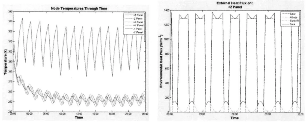
4-14 Comparison of the External Heat Fluxes on the -Z and +X Surfaces . . . .
4-15 Increasing the Conductance Value Between Surfaces . . . . 4-16 Temperature Response for a 2D Box with +Z in the Velocity Direction . . . 4-17 Temperature Response for a 2D Box in a Molniya Orbit . . . . 4-18 Test Case 4: 3D Six Panel Box with Internal Avionics Stack . . . . 4-19 Example of Individual Component Orientation . . . .
4-20 Temperature Response for a 3D Box with an Internal Avionics Stack . . . .
4-21 Temperature Limits for the +Z Panel and Avionics Stack . . . . 4-22 2D Surface Modeled in Thermal Desktop and ATMT . . . . 4-23 Thermal Desktop Validation of Test Case 1: Temperature at the Surface's
C entroid . . . . 4-24 3D Solid Rectangle Modeled in Thermal Desktop and ATMT . . . . 4-25 Thermal Desktop Validation of Test Case 2: Temperature at the Object's
C entroid . . . .
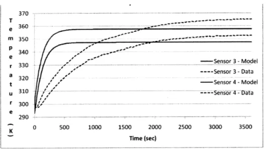
Final Model-Data Correlation... . . . .
CASTOR Structural Engineering Model and TVac Test Setup . . . . . Thermal Desktop Model of CASTOR Structure and TVac Test Setup TVac Test Model-Data Correlation . . . . ATMT Geometry Tab: 15 User Defined Input Categories . . . . ATMT Scenario Tab: 24 User Defined Input Categories . . . . ATMT Output Tab: Thermal Model Outputs and Sample Results . .
110 111 111 112 113 114 115 116 117 118 119 120
4-26 2D Six Surface Box Modeled in Thermal Desktop and ATMT
4-27 Thermal Desktop Validation of Test Case 3 . . . . 123
4-28 3D Six Panel Box with Avionics Stack Modeled in Thermal Desktop and ATMT.. . . .. . . .. . ... .... .. . ... . .. ... . . . . 125
5-1 ATMT at a Glance . . . . 129
5-2 ATMT Home Tab . . . . 131
5-3 ATMT Geometry Tab . . . . 133
5-4 Geometry Tab: Object Editor Panel . . . . 133
5-5 Geometry Tab: Object Property Table . . . . 135
5-6 Example of a Rectangular and Cylindrical Object . . . . .. 136
5-7 Geometry Tab: Check Facing Example . . . . 140
5-8 Geometry Tab: Geometric Configuration . . . . 141
5-9 Geometry Tab: Plot External Example . . . . 142
5-10 Geometry Tab: Hide Table Example . . . . 143
5-11 ATMT View Factors Tab . . . . 144
5-12 View Factors Tab: Matrix Editor Panel . . . . 144
5-13 View Factors Tab: View Factor Matrix . . . . 146
5-14 ATMT Conductance Tab. . . . .. 147
5-15 Conductance Tab: Conductance Table Editor . . . . 148
5-16 Conductance Tab: Conductance Matrix . . . . 149
5-17 ATMT Materials Tab . . . . 151
5-18 Materials Tab: Material Property Editor . . . . 152
5-19 Materials Tab: Surface Finish Editor . . . . 153
5-20 ATMT Scenario Tab . . . . 155
5-21 Scenario Tab: Orbital Parameters Panel . . . . 156
5-22 Scenario Tab: Scenario Panel . . . . 157
5-23 Scenario Tab: Initial Orientation Panel . . . . 158
5-24 Scenario Tab: Orbiting Body Panel . . . . 159
5-25 Scenario Tab: Simulation Data File Panel . . . . 161
5-26 Scenario Tab: Running the ATMT GUI . . . . 161
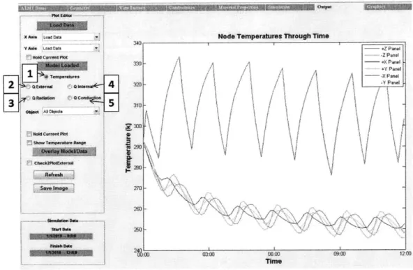
5-27 ATMT Output Tab . . . . 163
5-28 Output Tab: Output Plot Editor . . . .
A-1 CASTOR Structural Engineering Model Resistor Spreadsheet
B-1 TVac Chamber Internal Temperatures . . . . B-2 Model Data Correlation for the CASTOR Xenon Tank . .
B-3 Model Data Correlation for the CASTOR +Y Fin . . . .
B-4 ATMT Material Properties Database . . . .
B-5 ATMT Test Case Baseline Scenario. . . . . . . . . ..
B-6 Thermal Desktop On-orbit Display of a 2D Surface . . . .
B-7 Nanosatellite Thermal Test Bed . . . ...
B-8 Nanosatellite Thermal Test Bed: Side Panel Drawing . B-9 Nanosatellite Thermal Test Bed: Avionics Stack Drawing B-10 ATMT Results Plotted External to the GUI . . . .
. . . . 177 . . . . 178 . . . . 178 . . . . 179 . . . . 179 . . . . 180 . . . . 180 . . . . 181 . . . . 181 . . . . 182 164 175
List of Tables
1.1 Advantages and Disadvantages of Industry Standard Thermal Modeling
Pro-gram s . . . . . . . . .
1.2 Advantages and Disadvantages of Satellite Specific Thermal Algorithms
CASTOR Nanosat Component Temperature Constraints: . Thermal vs. Electrical Circuit Analogy . . . . Environmental Heat Sources: Average, Hot, and Cold Cases
Validation Results: Test Case 1 . . . . . . . . ..
Validation Results: Test Case 2 . . . . Validation Results: Test Case 3 . . . . View Factor Calculation Results: Version 1 . . . . View Factor Calculation Results: Version 2 . . . . ... . . . Initial Model Data Correlation Results . . . . Final Model Data Correlation Results . . . .
. . . . . 119 . . . . . 121 . . . . . 124 173 173 174 174 24 2.1 2.2 2.3 4.1 4.2 4.3 A.1 A.2 A.3 A.4
Nomenclature
AF Albedo Factor
ATMA Adaptive Thermal Modeling Architecture ATMT Adaptive Thermal Modeling Tool
CASTOR Cathode Anode Satellite Thruster for Orbital Repositioning CCDs Charged-Coupled Devices
CDD Capabilities Development Document CDIO Conceive Design Implement Operate CDR Critical Design Review
COEs Classical Orbital Elements CONOPs Concept of Operations
COTS Commercial Off the Shelf
CPD Capabilities Production Document DCFT Divergent Cusped Field Thruster DoD Department of Defense
EELV Evolved Expendable Launch Vehicle EHF External Heat Flux
EPS Electrical Power System
ESPA EELV Secondary Payload Adapter FAQ Frequently Asked Questions
FEM Finite Element Model FOV Field of View
FRR Flight Readiness Review
GN&C Guidance Navigation and Control GPS Global Positioning System
ICD Initial Capabilities Document
IJK Geocentric-equatorial Coordinate System IMU Inertial Measurement Unit
JPL Jet Propulsion Laboratory KDP Key Decision Point LEO Low Earth Orbit LOS Line-of-sight
MILspec Military Specification
MIT Massachusetts Institute of Technology MLB Motorized Light Band
MLI Multi-layered Insulation
MPPT Maximum Peak Power Tracker
NASA/JSC National Aeronautics and Space Administration/ Johnson Space Center OOH On-orbit Handbook
PDR Preliminary Design Review PDU Power Distribution Unit PPU Power Propulsion Unit
R.A.&Decl. Right Ascension and Declination SCT Spacecraft Control Toolbox
SEA Space Engineering Academy SEM Structural Engineering Model SMC Space and Missiles Systems Center
SR Steradian
SRR System Requirements Review STK Satellite Tool Kit
STP Space Test Program TCS Thermal Control System TD Thermal Desktop
TSS Thermal Synthesizer System TVac Thermal Vacuum
UCCS University of Colorado Colorado Springs uitable User Interface Table
UNP University Nanosatellite Program USAFA United States Air Force Academy VF View Factor
Chapter 1
Introduction
The driving force in the 2 1't century world of modern aerospace technology is the idea
of getting "more for less." This means that aerospace engineers must be able to design smarter, more efficient, and more reliable systems using less money, less time, and less manpower. These requirements have led to a culture shift in the aerospace industry from billion dollar school bus-sized spacecraft, traditionally produced by aerospace conglomer-ates, to multi-million dollar small satellites (smallsats) designed, built, and operated by small businesses and universities. Supporting the demands of this new "lean enterprise" generation of spacecraft will require innovative aerospace technologies and procurement techniques.
The acquisition of a smallsat follows a similar design sequence to that of a large satellite simply scaled to meet the mission objectives. The primary phases of the satellite acquisi-tion sequence are: concepacquisi-tion, design, build, testing, launch, and operaacquisi-tions. All phases inevitably are shortened and restructured in order to develop smallsats cheaper, faster and with less manpower. Smallsats take advantage of their size and relative importance by using either components designed in-house which are often non-space qualified hardware, or by purchasing commercial of the shelf (COTS) hardware. Often times only critical subsystems will have multiple inhibits or redundant components. The combination of un-proven hard-ware, fewer inhibits, and less redundancy introduces risk and the perception that smallsats are unreliable in the space environment.
program. The risks manifest themselves as on-orbit hardware and software failures due to the harsh environmental conditions in space. The space environmental conditions include: near zero gravity, magnetic fields, ambient temperature, vacuum, and particles (radiation, space debris, and charged particles) [18]. The ambient temperature, vacuum, and radiation effect can be combined into the space thermal environment. Rarely do thermal related issues lead to mission failure, but they do have a significant impact on system performance and reliability. For this reason a satellite's response to the space thermal environment is consistently an area of emphasis.
Many of the risk and reliability concerns can be overcome through extensive modeling and simulation of a satellite's behavior in the space environment. Innovative modeling and testing processes are allowing the transition from larger, more expensive satellites to smaller, cheaper, and more expendable satellite programs. In particular, the thermal modeling and testing tools and techniques used in smallsat programs have become a major area of research and are the motivation for this thesis.
Satellite thermal analysis requires modeling and testing of both the launch and space environments. This task is often complex, expensive, and time consuming. Sacrifices are made by testing specific components or areas of concern and using the results to validate the thermal models and analysis. Once validated, the model can be used to design a Thermal
Control System (TCS) that either passively maintains thermal equilibrium or is actively responsive to the changing thermal environment in space.
The existing thermal modeling tools fall into two categories: commercially available industry standard tools and satellite specific algorithms. Both have advantages and disad-vantages but neither is fully suited for a smallsat program. Bridging the gap between the commercially available industry standard tools and the satellite specific algorithms will re-quire a modeling architecture that is flexible to thermal modeling applications throughout all phases of the smallsat acquisition lifecycle. The Adaptive Thermal Modeling Architecture
(ATMA) presented in this thesis provides a modeling tool, model validation methodology,
and the model implementation techniques to satisfy the thermal modeling requirements and constraints of a smallsat program.
of ATMT was to simplify the thermal modeling process while offering functional tools and sufficient accuracy for a smallsat program. The modeling tool is flexible to numerous smallsat applications with the potential to model a variety of mission profiles. ATMT's user friendly interface allows an engineer to quickly develop a thermal model, run orbital simulations, and use the results to make important TCS design decisions. Ideally an engineer with little knowledge of satellite thermal design and control could use ATMT to predict, test, and understand a spacecraft's thermal response in order to meet the satellite's thermal requirements.
The ATMA modeling tools and techniques have been tested and validated using the MIT CASTOR satellite. Currently, ATMA is being tested on the MIT CASTOR and Exoplanet satellite's as well as the U.S. Air Force Academy's FalconSAT-6. The university smallsat arena provides the perfect setting to demonstrate the capability of new modeling architec-tures. In comparison to commercial or military space programs, university space research programs have relatively low budgets, short schedules, and inexperienced manpower. For these reasons, the thermal modeling techniques discussed in this thesis can be implemented and evaluated first at the university level and if successful, applied to any small satellite program.
1.1
Problem Statement
Currently the modeling tools and techniques used to simulate a satellite's thermal on-orbit lifecycle are geared toward programs with large budgets, extended schedules, and designated experts. Small satellite programs cannot afford large margins in these areas and as a result they frequently struggle and often fail due to thermal design complexities.
1.2
Thesis Motivation
Adapt the current thermal modeling tools and techniques to smallsat programs with low budgets, short schedules, and inexperienced engineers. Use ATMA to design and imple-ment an efficient, functional, and sufficiently accurate thermal modeling approach for small satellite applications.
1.3
Thermal Modeling Options
Spacecraft thermal modeling is used primarily for the design and evaluation of a space-craft's Thermal Control System (TCS) whose purpose is to ensure the survivability and performance of the payload and spacecraft subsystems. In the past, large space programs have relied on commercially available industry standard thermal modeling tools and highly skilled thermal engineers to model a spacecraft's on-orbit thermal response. Today, the scale of space programs is moving toward the small and nano-class range which require a different set of thermal modeling tools and techniques. Due to time, budget, and personnel constraints, many small satellite programs are moving toward satellite specific thermal al-gorithms for TCS design and analysis. This section compares the industry standard tools to the satellite specific algorithms to determine how well each is able to meet the thermal modeling requirements of a smallsat program.
Industry standard tools and satellite specific thermal algorithms each have distinct ad-vantages and disadad-vantages. The adad-vantages of using an industry standard tool are ac-curacy, modeling flexibility, heritage, and pre and post processing capabilities while the disadvantages are cost, modeling time, and complexity. Table 1.1 shows a summary of the advantages and disadvantages for industry standard thermal modeling programs.
Table 1.1: Advantages and Disadvantages of Industry Standard Thermal Modeling Pro-grams
Advantages
Accuracy Highly accurate: ±1 Kelvin
Flexibility Many ways to model the same thing; very detailed models
Heritage Proven to work; used for multiple mission applications
Pre/Post Processing Extensive construction, visualization, and analysis tools
Disadvantages
Cost ~0 $2k -+~ $1k per license per year
Time Time to learn software; time to build and test models
Complexity Multitude of variable parameters
Generic User starts from scratch; no baseline design
There are a variety of commercially available thermal-analysis software packages recom-mended for spacecraft applications [7].
" Thermal Desktop (TD) by Cullimore and Ring Technologies; TD requires AUTOCAD
" Thermal Synthesizer System (TSS) by SPACEDESIGN under license to NASA/JSC
" THERMICA by Network Analysis Inc. under license to ASTRIUM " FEMAP/SINDAG Modeling System by Network Analysis Inc. " IDEAS TMG Thermal Modeling System by MAYA
" ITAS by Analytix Corporation
" Thermal Analysis System by Harvard Thermal
Thermal Desktop (TD) is one of the most commonly used programs for smallsat ap-plications. As an extension to AutoCAD, TD offers a full computer aided design (CAD) modeling suite that allows the user to customize component geometries and orientations. TD offers an extensive array of tools that allow the user to specify material properties, surface finishes, and meshing dimensions. After constructing and orienting a series of com-ponents the user must define the contact method between each component. Finally, the user is able to create an on-orbit scenario for thermal analysis. Many flexible options allow the user to tweak the model through each step of the process. At times these options are overly complex adding ambiguity and uncertainty to the model. TD requires extensive training and an understanding of the heat transfer mechanisms in the space environment. However, a complete user's guide and technical support make TD an extremely useful commercial tool for small spacecraft thermal modeling.
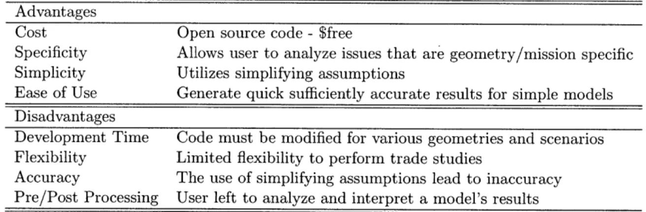
While platforms such as TD, Solidworks, and Abaqus certainly have the capacity and flexibility to accomplish a wide variety of thermal analyses, generating and testing a com-prehensive thermal model requires extensive time and user expertise. The satellite specific thermal algorithms are a means of generating sufficiently accurate results with less time and experience. Their advantages include lower cost, higher specificity, simplicity, and ease-of-use while their disadvantages include reduced flexibility, accuracy, and pre and post processing capabilities. Table 1.2 shows a summary of the advantages and disadvantages for satellite specific thermal algorithms.
Table 1.2: Advantages and Disadvantages of Satellite Specific Thermal Algorithms Advantages
Cost Open source code - $free
Specificity Allows user to analyze issues that are geometry/mission specific
Simplicity Utilizes simplifying assumptions
Ease of Use Generate quick sufficiently accurate results for simple models
Disadvantages
Development Time Code must be modified for various geometries and scenarios
Flexibility Limited flexibility to perform trade studies
Accuracy The use of simplifying assumptions lead to inaccuracy
Pre/Post Processing User left to analyze and interpret a model's results
The demand for smaller, better, cheaper satellites has lead to the development of many new professional and educational satellite modeling tools tailored toward smallsat commu-nity. Princeton Satellite Systems offers a professional commercially available integrated satellite design and analysis tool known as the Spacecraft Control Toolbox (SCT). The MATLAB-based SCT offers analysis tools for a variety of spacecraft systems with a focus on Guidance Navigation and Control (GN&C) applications.
Thermal modeling is offered as a module within SCT. The Thermal Module offers several very useful features however, it comes with the caveat that it is meant to "help GN&C analysts uncover potential thermal problems caused by GN&C activity," and not as a substitute for programs such as TD, Solidworks or Abaqus [14]. The thermal modeling tools allow the user to get a basic idea of the equilibrium temperatures at the satellite level. This means that temperatures are projected for a few key nodal points such as the Earth-facing side or Sun-facing side. Figure 1-1 shows a visual of a satellite modeled using SCT's thermal imaging function. The main limitation with the SCT Thermal Module is that the thermal algorithms are meant to provide a first order estimate of the temperatures. Smallsat thermal modeling beyond the concept study phase requires the ability to easily increase the number of components while modifying their geometry, spatial location, and operating parameters through time.
SatTherm is a MATLAB and Excel-based small spacecraft thermal analysis tool devel-oped by Cassandra VanOutryve in collaboration with the Mission Design Center at NASA Ames [24]. The goal of the SatTherm project was to develop a conceptual design phase tool
Figure 1-1: Spacecraft Toolbox Thermal Imaging Demo [14]
that could model the on-orbit temperature response for basic spacecraft configurations. The advantage of the SatTherm program is its ease-of-use and ability to perform quick trade studies on material properties and orbital scenarios.
The SatTherm program uses an Excel input file to run a series of thermal algorithms in MATLAB. The MATLAB algorithms generate the transient temperature and external heat flux results for an on-orbit simulation. The Excel input file allows the user to specify the shape (square box, hexagon, or octagon) and material properties of the spacecraft. All of the objects in SatTherm are modeled as 2D surfaces that both radiate and conduct heat to one another. The Excel input file also controls the on-orbit scenario parameters. These parameters include the simulation run-time, orbital elements, spacecraft orientation, and solar position.
The algorithms used in the SatTherm program were validated against TD with an accu-racy of ±4 Kelvin. SatTherm satisfies fulfills its purpose as a conceptual design and analysis tool. Unfortunately SatTherm is limited to a very narrow range of small spacecraft ther-mal modeling applications. The geometric constraints make it difficult to model spacecraft configurations that deviate from the three prescribed shapes and the 2D surface approach reduces the model's accuracy for truly 3D objects. While SatTherm is a great basis' for small spacecraft thermal modeling, several adaptations and extensions may be added to increase its functionality and its ability to meet the thermal modeling requirements of a smallsat program.
1.4
Research Gap Analysis
A plethora of good information was attained by evaluating and testing the various industry
standard thermal modeling tools and satellite specific thermal algorithms. As shown in Section 1.3, each tool had many strengths and only few weaknesses. However, through experience with two university smallsat programs it seems that spacecraft thermal modeling remains a daunting task for the inexperienced thermal engineer. As the 2007-2008 Chief Engineer for the U.S. Air Force Academy's FalconSAT-5 satellite and the 2008-2010 lead thermal engineer for the MIT CASTOR program, the author has witnessed many of the challenges associated with thermal modeling in smallsat programs.
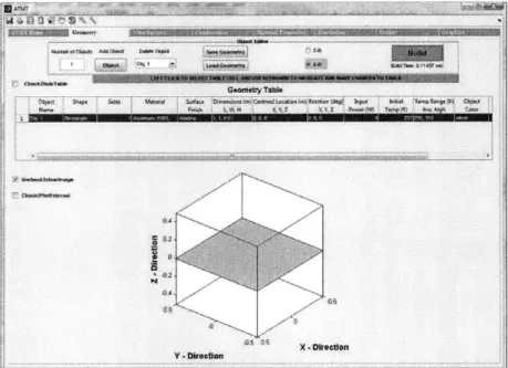
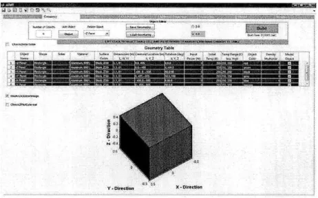
Due to the time, budget, and personnel constraints placed on smallsat programs, de-signing and testing a spacecraft's Thermal Control System (TCS) usually comes as a last priority. Instead, most smallsat programs rely on thermal modeling to predict and ana-lyze their spacecraft's on-orbit thermal performance. Thermal modeling occurs throughout multiple phases of a program from initial conception through testing and into the on-orbit operations [7]. The Adaptive Thermal Modeling Architecture (ATMA) presented in this thesis, is a set of techniques designed to address the thermal modeling requirements of each phase. The focus of this architecture is on the design, validation, and implementation of the Adaptive Thermal Modeling Tool (ATMT). ATMT is a MATLAB-based thermal modeling tool designed for smallsat applications. The goal of ATMT is not to replace the industry standard or satellite specific algorithms, but to supplement their use in the smallsat realm. ATMT can be used for thermal design, on-orbit modeling, and data analysis at the compo-nent, assembly, and vehicle levels. A description of each level is provided below along with examples from ATMT shown in Figure 1-2.
Levels
" Component - A component is a standalone functional unit that usually requires
an interface (mechanical, thermal, electrical etc.) to other units in order to oper-ate. Examples include a battery box, a structural panel, or a xenon propellant tank. Figure 5-6(b) shows an example of 3D cylindrical tank modeled in ATMT.
or more types of interfaces. Examples include the Electrical Power System (EPS), Thermal Control System (TCS) or the spacecraft structure. Figure 5-6(a) shows an example of satellite's box structure modeled in ATMT.
9 Vehicle - The vehicle includes all of the assemblies integrated into an independently controlled and operated system. The vehicle will undergo all integrated modeling and testing and will be launched as a payload using a launch system. The vehicle may or may not remain in communication with the ground and launch segments. Section 2.1 provides a description of the spacecraft hierarchy including large, small, nano, and cube sized satellites. Figure 1-2(c) shows an example MIT's CASTOR nanosat modeled in ATMT.
020.406
-0.4 05
Y - Direction
(a) Cylindrical Xenon nent Level) C
0
0, 0.2 X - Direction Tank (Compo-0 Y -Direction -0.5 05 X - Direction(b) Six Panel Box Structure (Assembly
Level)
01
X
-Direction
Y
-Direction
(c) Massachusetts Institute of Technology CASTOR Satellite (Vehicle Level)
Figure 1-2: ATMT Model Examples
(31 U.2
0,4
There are many ways to judge the performance of a thermal model and choosing the right metrics is done based on a program's requirements. Section 1.3 presented a comparison of the advantages and disadvantages of both industry standard thermal modeling programs and satellite specific algorithms. The advantages and disadvantages can be translated into a set of performance metrics for ATMT.
1. Cost - The goal is for ATMT to be free to educational institutions. A User's Manual and limited source code are available in Chapter 5 and Appendix C.
2. Accuracy -The accuracy metric is a measure of how closely the ATMT results match
the results from an industry standard tool. The accuracy goal is to attain temperature
responses with < 5% error and < 11 Kelvin absolute temperature difference. The
accuracy metric is a quantitative means of determining the capabilities and limitations of the ATMT program. Understanding the capabilities and limitations allows the thermal engineer to apply appropriate margins when necessary.
3. Usability - The usability metric is a measure of how well ATMT satisfies the ther-mal modeling requirements of a sther-mallsat program. Usability is comprised of a subset of metrics including model functionality, specificity, simplicity, and ease-of-use. The usability metric provides a qualitative means of determining the capabilities and lim-itations of the ATMT program.
(a) Functionality -As a preliminary design tool, ATMT must be flexible to
chang-ing designs and increaschang-ing levels of complexity. The functionality of ATMT is demonstrated by its ability to easily design a model, test a given scenario, and post-process the results. A discussion of ATMT's functionality is available in Section 4.4.
(b) Specificity - The specificity metric is a measure of how closely a model is tied to its source code. Highly specific algorithms will require the user to actually modify code in order to change the model. Clearly this limits the ability to perform trade studies and to implement design changes. On the other hand, non-specific programs often provide multiple means of designing the same model
- leaving it up to the user to know which approach is correct. ATMT takes the middle ground by allowing modifications to be made easily within a graphical user interface (GUI) environment while requiring that a consistent design process be followed in order to limit any ambiguity in the design.
(c) Simplicity - Simplicity in a model is critical for the preliminary design phases
where accuracy is balanced with the need to perform quick trade studies. ATMT utilizes a set of appropriate simplifying assumptions that reduce the extremely complex thermal processes to standard equations that are well understood and easily validated. While the simplifying assumptions will inevitably lead to some error, they allow an inexperienced thermal engineer to understand the processes that occur within the model.
(d) Ease-of-Use - The ease-of-use metric refers to how quickly the user is able to learn ATMT and how well ATMT meets a set of thermal modeling requirements. ATMT offers an extensive set of pre and post processing tools that were tailored specifically to address the thermal modeling requirements of a smallsat program. The ATMT User's Manual describes these features with examples of potential applications.
1.5
Thesis Overview
The layout of this thesis is meant to take the reader through the motivation, justifica-tion, and demonstration of how the Adaptive Thermal Modeling Architecture (ATMA) was
developed, tested, and verified.
Chapter 2 describes the background information and mathematics utilized in the Adap-tive Thermal Modeling Tool (ATMT). This chapter provides a quick yet comprehensive
summary of the thermal modeling basics.
Chapter 3 takes the reader through each element of the three phase ATMA modeling process. Section 3.1 introduces the ATMT model structure and several of its key thermal al-gorithms while Section 3.2 addresses the ATMA model-to-model and model-data correlation techniques used to validate the ATMT program.
Chapter 4 introduces the ATMT background methodology and simplifying assumptions as well as the simulation's inputs and outputs. Section 4.4 discusses ATMT's functionality and provides several test cases and analyses demonstrating the ATMT modeling techniques. The test case results are then validated using Thermal Desktop. The chapter is concluded
by a summary of the usability tests that were conducted at the U.S. Air Force Academy.
Chapter 5 provides a complete ATMT User's Manual describing how to utilize ATMT for spacecraft thermal modeling purposes. The manual takes the reader through the six tabs of the ATMT GUI providing examples for each function and techniques to aid in the modeling process.
Chapter 6 presents a summary of the thesis, contributions to the field, and suggested future work.
Chapter 2
Background
Designing and modeling an effective spacecraft Thermal Control System (TCS) requires an understanding of the top-level mission objectives as well as the physical interactions between components and their operational environment. The mission objectives translate into the system, assembly and component-level thermal control requirements. Thermal control is accomplished through a variety of methods both passive and active that are used to maintain component temperatures within their operational or survival range.
The scope of this thesis is on TCS design and modeling techniques for small and nano satellite programs. Most small and nano-class satellites strive to use passive thermal con-trol. Passive control can be achieved through the use of special surface finishes and proper orientation of heat producing and heat rejecting components. Some spacecraft components are extremely sensitive to changes in their thermal environment and may require addi-tional active control mechanisms to meet their thermal requirements. Active control may be achieved by maintaining a spacecraft's attitude orientation with respect to external heat sources or by using heating and cooling devices to maintain component temperature ranges. This chapter provides the background math and processes required to understand on-orbit thermal modeling. Beginning with an overview of the spacecraft size hierarchy in Section 2.1, Chapter 2 goes on to describe the orbital mechanics, heat transfer processes, and material properties used for transient thermal modeling in the Adaptive Thermal Modeling Tool (ATMT).
2.1
Spacecraft Size Hierarchy
The size-name relationship for spacecraft follows primarily from the volume of the structure. The major breakpoint is generally defined between primary and secondary payloads, where the primary payload on a given mission will often be physically larger, more expensive, and more complex than any of the secondary payloads. Another spacecraft size distinction is often associated with the deployment mechanism and in turn the mass of the spacecraft. Using these two size-name distinctions, spacecraft sizes can be broken into four categories: large satellites, small satellites (smallsats), nano satellites (nanosats), and cube satellites (cubesats).
" Large Satellites - A spacecraft weighing more than 181 kg or being deployed using
a Motorized Light Band (MLB) larger than 15 inches in diameter [5]. Large satellites will range from 181 kg and roughly a cubic meter in volume, to over 10, 000 kg and the size of a school bus. Large Satellites will serve as the platform for either one large or several small technical payloads 1. Milstar-5 shown in Figure 2-1(a) is an example of a large satellite.
* Smallsats -A spacecraft weighing less than or equal to 181 kg and greater than 50 kg. These spacecraft are often called ESPA (EELV Secondary Payload Adapter) class
spacecraft and will adhere to a very specific set of launch requirements as outlined in the ESPA User's Guide [22]. A smallsat will usually carry one primary payload and may have several supporting secondary payloads. STPSat-2 shown in Figure 2-1(b) is an example of a smallsat.
" Nanosat and Cubesat - Derived from the University Nanosatellite Program (UNP) requirements [6], a nanosat is any spacecraft smaller than 50 kg that is separated from the launch vehicle independent of the primary or other secondary payloads. We will assign a lower bound of 4 kg, which is the maximum mass for the standard 3 unit
(3U) cube satellite (cubesat). A nanosat is very similar to a smallsat in that they will
generally carry one or more small payloads. A cubesat is a standardized 1 -+ 3 unit
assembly where each unit is a 10x10x10 cm box containing one or more subsystems. Figure's 2-1(c) and 2-1(d) show examples of MIT's CASTOR nanosat and Space Data System's ISR-3.
(a) Milstar-5 in the Factory (Large (b) STPSat-2 in the Clean Room (Small
Satellite) [15] Satellite) [2]
(c) MIT CASTOR Engineering Model (d) Space Data Systems ISR-3
(Cube-(Nanosatellite) sat) [16]
2.2
Small and Nanosat Thermal Control Systems
The primary objective of the TCS is to keep the spacecraft's components within their required temperature range throughout their lifecycle. Most components are given two temperature ranges; operational and survival. The operational temperature range is the most stringent range that must be maintained while the component is operating to achieve its intended performance. The survival range is the temperature range associated with the non-operating phase of a component's lifetime and provides the maximum and minimum temperatures the component can withstand without being rendered inoperable. Most com-ponents are designed to operate nominally at room temperature 273 ±30 Kelvin. Mission constraints may require a particular to component to remain either extremely cold or ex-tremely hot, or even to maintain a very narrow temperature range in order to minimize shock due to thermal cycling. Table 2.1 shows an example of the temperature constraints
used for the MIT CASTOR nanosat.
Table 2.1: CASTOR Nanosat Component Temperature Constraints:
Component Operating Range (K) Survival Range (K)
Battery 273 -+ 313 263 -+ 318 MPPT 233 - 333 228 - 353 PPU 233 -+ 358 228 -+ 368 PDU 218 -+ 373 208 - 383 Solar Cells 183 -+ 433 173 -+ 443 GPS 253 - 323 243 - 333 IMU 233 -+ 358 218 -+ 358 Rxn Wheel 253 -+ 333 238 -+ 343 Camera 223 -+ 343 213 -+ 253 Payload 258 -+ 473 243 -+ 358 Temp Sensors 228 - 388 218 - 398
2.2.1
Thermal Margin
A thermal engineer's primary responsibility is to ensure that component temperature
re-quirements are met throughout all stages of the satellite's operational lifecycle to include: launch, separation, comissioning, normal operations, safe-modes, and decomissioning. To
accomplish this task the thermal engineer must accurately project the worst case hot and cold temperature range for the spacecraft. All spacecraft components have a survivable and operational temperature range and exceeding either at the wrong time can be detrimental to the mission. Modeling a spacecraft's on-orbit thermal response is a critical risk-reduction step in the design phase.
With all of the simplifying assumptions used in thermal modeling and the uncertainties associated with thermal analysis in general, it is nearly impossible to fully characterize a satellite's on-orbit thermal response. Adding margin to the TCS design is an essential means of risk-reduction. Figure 2-2 shows the JPL/NASA thermal margin methodology
used for hardware testing and flight operations [7]. Their approach has been adapted by
military space programs and is the standard used in ATMA. The diagram shows several layers of margin that should be applied to the thermal model's predicted temperature range throughout the satellite acquisition process.
Thermal
reliability
margin (20*C)
FA thermal
reliability margin (5*C)
Thermal design margin
Worst case
Allowable
Flight
Protoflight/
hot/cold
flight
acceptance
qualification
predicted
temperature
temperature
temperature
temperature
range
range
range
range
Thermal design margin
FA thermal reliability margin (500)
Thermal reliability margin (15*C)
Figure 2-2: Thermal Margin Terminology for JPL/NASA Programs [7]
Even after a satellite's worst case hot and cold temperature ranges are modeled and validated through TVac testing, a thermal margin of ±11 K is added to account for the
numerous uncertainties and assumptions made in the thermal analysis. On top of that is a flight acceptance margin that is required for acceptance testing of flight hardware. Finally, a thermal reliability margin is applied for the rigorous standards used in thermal qualification testing. The ATMT accuracy requirement discussed in Section 1.4 is based on JPL/NASA's most stringent ±11 K thermal margin.
2.3
Keplerian Orbit
There are several ways to define a spacecraft's orbit and position in space. The thermal modeling techniques used in the Adaptive Thermal Modeling Tool (ATMT) are based on the six Keplerian element's or Classical Orbital Elements (COEs). The six COEs are: the semi-major axis (a), eccentricity (e), inclination (i), longitude of ascending node Q),
argument of periapsis (w), and the true anomaly (v) [18]. Using these COEs, one can define
the size, shape, and orientation of the orbit as well as the position of the spacecraft within that orbit. Figure 2-3 shows how the inclination, longitude of ascending node, argument of periapsis, and the true anomaly are defined with respect to an orbital plane of reference.
Figure 2-3: Classical Orbital Elements [21]
element and its mathematical derivation can be found in the textbook Understanding Space
by Jerry Jon Sellers and Associates [181.
1. Semi-major axis (a) - The semi-major axis is used to determine the size of an orbit and is related to the specific mechanical energy or the orbit. The semi-major axis is found using Equations 2.1 and 2.2.
a =(2.1)
2e
2
=
-.
I
(2.2)
2 ||Rsc l
where p (3.986x10⁵ km3
/S2) is the gravitational parameter for Earth and e (km 2/ 2) is the specific mechanical energy of the orbit. The specific mechanical energy is found from the magnitudes of the spacecraft's position Rsc (km) and velocity Vsc (km/s) vectors.
2. Eccentricity (e) - The eccentricity is a measure of the shape of an orbit. Eccentricity
ranges indicate the type of orbit with e = 0 indicating a circular orbit, 0 < e < 1 an
ellipse, e = 1 a parabola, and e > 1 a hyperbola. The eccentricity can be calculated
directly from the semi-major axis using Equation 2.3 [18].
2c
e = -- (2.3)
2a
where c (km) is half of the orbital focal length (0 km for circular orbits), and a (km) is the semi-major axis. Alternatively the eccentricity can be determined from the spacecraft's position and velocity vectors Rsc and Vsc as shown in Equation 2.4.
1 1 -2 P ) -C_ -S. -
-s=- ||Vsc||-
..
Rs-Rs
-Vsc)VscV
(2.4)
p |Rsc||
3. Inclination (i) - The inclination is the angle (deg) from the plane of reference to the orbital plane as shown in Figure 2-3. Inclination may range from 0' < i < 180'. An
inclination of 0' < i < 900 indicates a direct or prograde orbit, 90' < i < 180' is an
indirect or retrograde orbit and i = 90' is a polar orbit. The inclination is the first of
three parameters (i, Q, and w) needed to define the orientation of an orbit is space.
4. Longitude of Ascending Node (Q) -The longitude of ascending node also referred to as the right ascension of the ascending node (RAAN), is the second parameter used in determining the orbit's orientation. RAAN is the angle (deg) from the reference direction ('y) or (I) in the geocentric-equatorial (IJK) frame, to the ascending node of
the orbit. Figure 2-3 shows Q as it is measured from the reference direction -y to the
ascending node in the plane of reference.
5. Argument of Periapsis (w) - The argument of periapsis or argument of perigee (argP) is the third element used to describe an orbit's orientation in space. The argument of perigee is the angle (deg) between the ascending node line and perigee of the orbit measured in the orbital plane.
6. True Anomaly (v) - With the size, shape, and orientation of the orbit defined, all that is left is to determine the spacecraft's position within its orbit. The true anomaly is the angle (deg) from perigee to the position of the spacecraft within its orbit. Figure 2-3 represents the spacecraft as the "Celestial Body" with true anomaly
measured in the orbital plane in the direction of motion.
2.3.1 Spacecraft Position and Velocity
There are several methods for determining a spacecraft's geocentric-equatorial position Rsc
(km) and velocity
9sc
(km/s) vectors. David Vallado, author of Fundamentals ofAstro-dynamics and Applications, offers a variety of potential algorithms as well as open-source
code for each method [23]. One of the more common methods of determining the Rsc and
Vsc vectors, and the method implemented in the SatTherm orbital propagation algorithm (geocen-rv.m), is to use the COEs discussed in Section 2.3. Given a, e, i, i, W, and time (t), it is possible to propagate the Rsc and Vsc vectors through each time step of the sim-ulation [243. The Rsc and Vsc vectors shown in Figure 2-4 are used to fix the spacecraft's
attitude on-orbit as well as determine if the spacecraft is in the Sun or eclipse at each time step.
-
~
~
P - - scRx I
Ra
R
Figure 2-4: Determining the Position and Velocity Vectors
2.3.2
Spacecraft Attitude On-orbit
A spacecraft's attitude on-orbit is a description of its body orientation in the
geocentric-equatorial (IJK) coordinate frame. In thermal modeling, a spacecraft's orientation affects how it will absorb heat from external sources such as the Sun and Earth. In actuality, each surface on every component has its own relative attitude that must be rotated from the surface's body frame to the IJK frame. The orientation of each surface with respect to one another governs how heat is radiated internally within the spacecraft and externally to cold space. Fixing a spacecraft's attitude orientation in space is done by choosing a desired pointing direction, selecting the primary axis (+X, +Y, or +Z) to point along that direction, and rotating all of the surfaces from the body frame to the IJK frame accordingly. Some of the most common attitude orientations include: Sun-facing, nadir-facing, velocity-facing, and fixed right ascension and declination (R.A. & Decl.).
Establishing a spacecraft's orientation requires fixing two axes, the primary and a sec-ondary, along two known vectors in inertial space. As discussed in Section 2.3.2, the space-craft's position Rsc and velocity Vsc vectors are the most obvious choices and are used to define the nadir and velocity facing orientations. For the Sun-facing and R.A. & Decl. orientations, two new vectors S and Hsc are used. Where S (km) is the spacecraft to Sun vector and Hsc (km) is the vector perpendicular to the orbital plane at the position of the
satellite. Figure 2-5 shows these four vectors in the IJK frame.
Vsc
Hsc
SCII
Rsc,
Figure 2-5: Spacecraft Attitude On-orbit
Using these four vectors the primary body axis is aligned with the chosen orientation by setting it equal to the vector's magnitude. The secondary axis is then set to the magnitude of a second chosen direction with the third axis completing the right-hand rule. If needed, the spacecraft may be rotated off-axis by an additional amount or it may have an angular rotation about one or more axes. Equation 2.5 shows how to align the +Z, +X, and +Y body axes for a +Z Sun-facing orientation. The secondary axis +X is aligned in the velocity direction with +Y determined by the cross product of the +Z and +X axes.
S
Zbody = - (2.5a)
cross(Ni,
Zbody)
Xbody =--(2.5b)
|cross
(H, Zb,,dy)Ybody = cross
(Zbody,
Xbody) (2.5c)2.4
Heat Transfer in the Space Thermal Environment
The thermal environment in space directly impacts a spacecraft's performance on-orbit by controlling how energy, in the form of heat, is transferred to and from a spacecraft. Oper-ating in the thermal-vacuum environment of space negates convection making conduction
and radiation the dominant modes of heat transfer in space2
Conduction and radiation heat transfer obey both the first and second laws of thermo-dynamics. The first law requires that the rate of energy transferred into a system be equal to the rate of energy leaving the system such that there is a conservation of energy. The second law states that energy will be transferred in the direction of decreasing temperature
[3]. These laws are implemented through the general heat-transfer equation which includes
both the internal and external sources of heat described in Section 2.6 [7].
OT
pC, a = V. (K - VT) + q(T, t) Energy rate per unit volume (2.6)
where p (kg/m 3) is the material's density, C, (J/kgK) is the material's specific heat, V
(1/m) is the gradient operator, K (W/mK) is the conductivity tensor, T (K) is the tem-perature, t (sec) is time, and q (W/m) is the heat input source term. Equation 2.6 forms the basis for both conduction and radiation heat transfer described in Sections 2.5 and 2.6 respectively.
2.5
Conduction
Conduction is heat transfer from the more energetic higher temperature particles of a body to the less energetic cooler particles [3]. This implies that a thermal gradient must ex-ist across the body for conduction to occur. The material properties and geometry of a component will play a significant role in its ability to conduct heat. For simplicity the
ID conduction equation is used in this thesis to model conduction through thin sheets of
material. Most spacecraft components are built from thin sheets of material to minimize their mass so the ID conduction equation is a valid approximation. Equation 2.7 shows the
1D conduction version of the heat-transfer equation.
dT
Qcond = ICpAT = -kA (2.7)
dx
2
Convection requires a medium such as a gas or liquid for heat transfer to occur. Space is assumed to be a perfect vacuum with negligible atmospheric density. Atmospheric density increases with decreasing altitudes. For extremely low altitudes the affects of convection may no longer be assumed negligible.
![Figure 1-1: Spacecraft Toolbox Thermal Imaging Demo [14]](https://thumb-eu.123doks.com/thumbv2/123doknet/13865483.445892/25.918.242.686.109.320/figure-spacecraft-toolbox-thermal-imaging-demo.webp)
![Figure 2-3: Classical Orbital Elements [21]](https://thumb-eu.123doks.com/thumbv2/123doknet/13865483.445892/39.918.263.663.637.998/figure-classical-orbital-elements.webp)