The Air Quality and
Health Impacts of Aviation in Asia
by
In Hwan Lee
B.S. Engineering Physics
University of California, Berkeley, 2010
SUBMITTED TO THE DEPARTMENT OF AERONAUTICS AND
ASTRONAUTICS IN PARTIAL FULFILLMENT OF THE REQUIREMENTS
FOR THE DEGREE OF
MASTER OF SCIENCE IN AERONAUTICS AND ASTRONAUTICS
AT THE
MASSACHUSETTS INSTITUTE OF TECHNOLOGY
SEPTEMBER 2012
© 2012 Massachusetts Institute of Technology. All rights reserved
Signature of Author………...
Department of Aeronautics and Astronautics
September 2012
Certified by………...
Steven R.H. Barrett
Assistant Professor of Aeronautics and Astronautics
Thesis Supervisor
Accepted by………...………...
Eytan H. Modiano
Professor of Aeronautics and Astronautics
Chair, Graduate Program Committee
The Air Quality and
Health Impacts of Aviation in Asia
byIn Hwan Lee
Submitted to the Department of Aeronautics and Astronautics On August 23, 2012 in Partial Fulfillment of the Requirements for the Degree of Master of Science in
Aeronautics and Astronautics
at the Massachusetts Institute of Technology
ABSTRACT
Aviation in Asia is growing more rapidly than other regions around the world. Adverse health impacts of aviation are linked to an increase in the concentration of particulate matter smaller than 2.5 μm in diameter (PM2.5). This thesis aims to quantify the regional-scale health impacts of
aviation in Asia by modeling the air quality in Asia and applying Concentration-Response Functions (CRFs) to the aviation-attributable PM2.5 perturbations.
In order to quantify the perturbation to the ambient air quality due to aviation emissions, the Community Multiscale Air Quality (CMAQ) model—a regional-scale chemical transport model—is utilized after its performance is evaluated in predicting ambient PM2.5 concentrations.
Aviation emissions for 2006 are from the Aviation Environmental Design Tool (AEDT), and background emissions for 2006 are generated using a combination of four Asian and global emissions inventories.
A domain average increase of approximately 15ng/m3
in annual PM2.5 is observed due to full
flight aviation emissions, while Landing and Takeoff (LTO) cycle emissions account for an increase of approximately 0.75ng/m3. Calculations using two different CRFs used by the EPA
and the WHO estimate the following amount of aviation-attributable premature mortalities in Asia: 9400 (using the EPA CRF) or 6400 (using the WHO CRF) in the full flight scenario, and 550 or 390 in the LTO cycle scenario. Finally, comparisons to the global-scale model simulation results show consistent spatial patterns of air quality perturbations, while the regional-scale model estimates approximately 1.4 times the number of mortalities obtained from corresponding global-scale studies.
Thesis Supervisor: Steven Barrett
Acknowledgements
I would like to first thank my advisor, Professor Steven Barrett, for his support. Ever since my arrival at MIT, he has provided me with guidance and advice for my classes, research, and future career. I’m very grateful that he made himself approachable and available for his students, even with an unimaginably busy schedule. Without his help and encouraging words every week, my work at MIT wouldn’t have been the same.
I also would like to sincerely appreciate the mentorship and friendship of Dr. Steve Yim. The time I got to spend with him—whether in his office during the week or on the soccer field on Sundays—was fun and helpful. From project setup to result post-processing, his advice and guidance has touched every bit of my research.
Also, I would like to thank my fellow researchers at the MIT Laboratory for Aviation and the Environment. Numerous discussions and lunch runs with Akshay, Jamin, Gideon, Fabio, Chris, Sergio, and Philip will be missed dearly. Thanks also to Dr. Robert Malina, Dr. Christoph Wollersheim, and Dr. Alex Mozdzanowska for excellent leadership.
I want to express my sincere appreciation for HongSeok Cho, my friend and brother in Christ. Without his support, I would not have been able to withstand some of the toughest times of my stay at MIT. The tears and the joy we got to share together will be remembered and treasured. I’m extremely grateful for my family, whose overwhelming love and support for me could not be hindered even by the three-hour time zone difference. Without them, I wouldn’t have been able to come this far.
Lastly and most importantly, I would like to thank God for His everlasting and overwhelming love for me. I am here today, only by His grace. Soli Deo gloria!
Contents
LIST OF FIGURES………. 7
LIST OF TABLES………... 8
LIST OF ACRONYMS………... 9
CHAPTER 1
INTRODUCTION………...11
1.1
The Air Quality Impacts of Aviation………...11
1.2
Motivation—Regional Air Quality Impacts of Aviation in Asia…… 12
1.3
Thesis Outline………. 13
CHAPTER 2
MODEL SETUP………...…….………... 15
2.1
The CMAQ Model………... 15
2.2
Modeling Domain………... 16
2.3
Inputs to CMAQ……….. 19
2.3.1
Meteorology………... 19
2.3.2
Gridded Emissions………... 21
2.3.3
Initial Conditions & Boundary Conditions…………... 22
2.3.4
Others………... 22
2.4
Performance Evaluation……….. 23
2.4.1
Statistical Parameters for Performance Evaluation………. 24
2.4.2
Meteorology……….…... 25
2.4.3
Air Quality………..………. 28
CHAPTER 3
BACKGROUND EMISSIONS……...………... 30
3.1
Emissions Inventories………. 30
3.1.1
TRACE-P Emissions………... 31
3.1.2
INTEX-B Emissions………... 32
3.1.3
NH
3(Ammonia) Emissions………... 33
3.1.4
Shipping Emissions………...…….…. 34
3.2
Methodology………... 35
3.2.1
Horizontal Allocation……….. 36
3.2.3
Temporal Variation……….. 40
3.2.4
Chemical Speciation……….... 42
3.2.5
Sectoral Emissions………... 44
3.3
Uncertainty in Background Emissions……….... 45
CHAPTER 4
AVIATION EMISSIONS………... 47
4.1
Aviation Scenarios………. 47
4.1.1
Landing and Takeoff (LTO) Emissions………... 48
4.1.2
Ultra Low Sulfur (ULS) Fuels………... 49
4.2
AEDT 2006………... 50
4.2.1
Assignment to the CMAQ Grids……….……….... 50
4.2.2
Uncertainty in the Aviation Emissions……….... 54
CHAPTER 5
RESULTS………...… 55
5.1
Air Quality Impacts……….… 55
5.1.1
Constituents of PM
2.5………... 55
5.1.2
Spatial Distribution of Aviation-Attributable PM
2.5…….... 56
5.2
Health Impacts……….... 59
5.2.1
Health Impacts of PM
2.5Exposure………... 59
5.2.2
Premature Mortality Results……….... 61
CHAPTER 6
CONCLUSION………... 63
6.1
Summary………. 63
6.2
Limitations & Future Work………. 64
BIBLIOGRAPHY……….. 66
APPENDICES……….... 75
Appendix A CMAQ Model Build Parameters..………... 75
Appendix B
List of Emission Species…....………... 76
Appendix C
NMVOC Speciation for Background Emissions...………..77
List of Figures
Figure 2-1: The horizontal modeling domain……… 16
Figure 2-2: Vertical layer distribution………... 18
Figure 2-3: Spatial representation of the ocean file………... 23
Figure 2-4: Soccer goal plot of meteorology model performance evaluation ....……….. 27
Figure 2-5: Soccer goal plot of air quality model performance evaluation………...… 29
Figure 3-1: Black carbon emissions from TRACE-P large point source locations………... 31
Figure 3-2: Definition of inventory domain (for TRACE-P and INTEX-B)………. 33
Figure 3-3: Global shipping emissions: NOX (annual sum)………... 34
Figure 3-4: Ammonia emissions before (top) and after (bottom) horizontal allocation……….... 37
Figure 3-5: INTEX-B NOX emissions before (top) and after (bottom) horizontal allocation…... 37
Figure 3-6: Monthly profiles used in this thesis……….... 41
Figure 3-7: Diurnal profiles of various emission sources (a) and weekday transportation………... emissions (b)………... 42
Figure 3-8: PM2.5 speciation profiles (percent by mass) from the SMOKE model………... 43
Figure 3-9: Yearly Asian emission of combustion-related species by sector (tonnes/yr)………. 45
Figure 4-1: Altitude above ground level (AGL) vs. above field elevation (AFE)………. 49
Figure 4-2: A vertical sum of fuelburn (in kg) in the modeling domain for 2006………. 51
Figure 4-3: Amount of fuelburn (in kg) allocated in each vertical layer for 2006……… 51
Figure 5-1: Aviation-attributable domain-average annual PM2.5 (μg/m 3 )……….. 56
Figure 5-2(a): Change in annual average PM2.5 concentration due to aviation in Simulation #1.. 57
Figure 5-2(b): Change in annual average PM2.5 concentration due to aviation in Simulation #2.. 57
Figure 5-2(c): Change in annual average PM2.5 concentration due to aviation in Simulation #3.. 58
Figure 5-2(d): Change in annual average PM2.5 concentration due to aviation in Simulation #4.. 58
List of Tables
Table 2-1: Equations used for various statistical parameters………. 24
Table 2-2: Statistical parameters obtained for temperature at 2m (T2)………. 26
Table 2-3: Statistical parameters obtained for wind speed at 10m (WSPD10)………. 26
Table 2-4: Statistical parameters obtained for O3 concentration at ground……….. 28
Table 2-5: Statistical parameters obtained for PM2.5 concentration at ground………...28
Table 2-6: Statistical parameters obtained for PM10 concentration at ground………...28
Table 3-1: Percentage growth of anthropogenic emissions (annual) in China……….. from 2001 to 2006………... 32
Table 3-2: A summary of the four emissions inventories used in this thesis……… 35
Table 3-3: Unit and stack parameters of power plants in Beijing……….. 39
Table 4-1: Different modeling scenarios simulated in this thesis……….. 47
Table 4-2: Domain sum of AEDT emissions for Asia and the whole world………. 52
Table 4-3: UK airport LTO emissions with uncertainty ranges as percentage of the median…... 54
Table 5-1: Premature mortalities using the EPA (WHO) CRF, rounded to nearest ten………….61
List of Acronyms
ACE-Asia Asian Pacific Regional Aerosol Characterization Experiment AEDT Aviation Environmental Design Tool
AFE Above Field Elevation
AGL Above Ground Level
AMET Atmospheric Model Evaluation Tool AORGP Primary Organic Aerosols
BC Black Carbon
CB05 Carbon Bond 2005
CMAQ Community Multiscale Air Quality CRF Concentration Response Function CTM Chemical Transport Model
EDGAR Emissions Database for Global Atmospheric Research
EI Emission Index
EPA Environmental Protection Agency
FB Fuelburn
FNL Final operational global analysis FSC Fuel Sulfur Content
GBD Global Burden of Disease GDP Gross Domestic Product GEIA Global Emissions Initiative
GEOS-Chem Goddard Earth Observing System-Chemistry GRUMP Global Rural-Urban Mapping Project
HC Hydrocarbon
INTEX-B Intercontinental Chemical Transport Experiment-Phase B
IoA Index of Agreement
JPROC Photolysis rate processor for CMAQ LTO Landing and Take-Off
MCIP Meteorology-Chemistry Interface Processor NASA National Aeronautics and Space Administration NCEP National Center for Environmental Protection NMB Normalized Mean Bias
NME Normalized Mean Error
NOX Oxides of nitrogen
OC Organic Carbon
PBL Planetary Boundary Layer
PBL Planbureau voor de Leefomgeving (Netherlands Environmental Assessment Agency)
PEC Primary Elemental Carbon
PM Particulate Matter
PM2.5 Particulate matter < 2.5 μm in diameter
PM10 Particulate matter < 10 μm in diameter
PMFINE Unspecified PM2.5
PMC Coarse Particulate Matter
PMFO Fuel Organics Particulate Matter PMNV Non-Volatile Particulate Matter PNO3 Primary Nitrate Aerosol
POA Primary Organic Aerosol PRD Pearl River Delta
PSO4 Primary Sulfate Aerosol
PSU/NCAR MM5 Fifth Generation Pennsylvania State University / National Center for Atmospheric Research Mesoscale Modeling
R Correlation coefficient
RAINS-Asia Regional Air Pollution Information and Simulation Asia
RSM Response Surface Model
SMOKE Sparse Matrix Operator Kernel Emissions
SOX Oxides of sulfur
TRACE-P Transport and Chemical Evolution over the Pacific T2 Temperature at 2m above ground
ULS Ultra Low Sulfur
WHO World Health Organization WPS WRF Preprocessing System WRF Weather Research and Forecasting WSPD10 Wind speed at 10m above ground
1 Introduction
Aviation, with its ability to provide a rapid worldwide transportation network, is a significant contributor to the world economy. The aviation industry supported approximately 3.5% of global gross domestic product (GDP) and 56.6 million jobs worldwide in 2010 [1]. The economic impacts of aviation will likely become more significant in the future, with global aviation activity projected to grow at an average of approximately 5% per year until 2030 [2, 3, 4]. While this rapid growth in aviation activity is expected to increase the economic benefits of aviation, it will also amplify the environmental impacts of aviation. Thus, policymakers face a challenge in efforts to optimize the balance between economic benefits and environmental damages of anticipated growth in aviation activity.
1.1 The Air Quality Impacts of Aviation
Aviation can affect the environment by emitting air pollutants into the atmosphere, causing degradation of air quality. Air quality impacts of aviation can vary from local scale impacts in the vicinity of airports to regional and global scale impacts via intra- and intercontinental cruise emissions. The focus of this thesis is to analyze the regional air quality impacts of aviation in Asia.
The degradation of air quality poses a threat to human health; in particular, health impacts due to a long-term exposure to particulate matter smaller than 2.5 μm in aerodynamic diameter (PM2.5)
is found to outweigh the impacts from other species [5]. Aviation PM2.5 that is directly emitted
from an engine or formed immediately after exiting an engine is considered primary, whereas secondary particulate matter is formed through complex atmospheric chemical reactions and physical processes of emitted PM precursor species (such as NOX, SOX, and hydrocarbons) [6].
Both primary and secondary PM contribute to adverse air quality perturbations; thus health impacts of aviation could be quantified by taking measurements of the aviation-attributable PM2.5
concentrations. These PM species, however, are also emitted from non-aviation anthropogenic sources, such as power generation, automobile emissions, and industrial combustion; therefore, it is a difficult to experimentally distinguish the aviation-attributable particulate matter from the
non-aviation PM, except in the locality of airports. Due to this difficulty, air quality models are generally used for impacts assessment, particularly at the regional and global scale, and policy analyses in order to attribute PM to sources.
Simultaneously occurring physical and chemical processes in the atmosphere makes it extremely complex to model the relationship between emission fluxes and ambient concentrations of air pollutants such as various PM2.5 species. Thus, atmospheric models that can capture the effects of
emission patterns, meteorology, chemical transformations, and removal processes are essential to understanding the atmospheric system as a whole [7].
The Community Multiscale Air Quality (CMAQ) and GEOS-Chem models are some of the Chemical Transport Models (CTMs) often used to model and understand the relationship between the emission patterns and the consequent effects in ambient concentrations of chemical species in the atmosphere. GEOS-Chem, a global-scale CTM, was utilized in previous studies to quantify the global air quality impacts of aviation [8, 10] with a horizontal resolution of 4° × 5°. CMAQ, on the other hand, was employed to study regional-scale air quality impacts of aviation in the United States [12, 13] and in Europe [14], with a finer horizontal resolution of 36 km and 45 km, respectively.
1.2 Motivation—Regional Air Quality Impacts of Aviation in Asia
Aviation-attributable health impacts in Asia are of growing significance for a few reasons. First, growth in aviation activity in Asia—largely led by China and India—is expected to outpace growth from all other regions in the world. China currently is the second largest market for new airplanes and the demand for air travel to, from, and within China is expected to grow at about 7.6% annually [1, 2]. India is expected to be the fourth largest market for new airplanes in the next 20 years, and is expected to experience the world’s fastest annual growth rate in aviation activity at approximately 8% to 9% [2, 3].Also led by China and India, the population in Asia is a significant fraction of the world’s population. The United Nations estimates the population in Asia to be approximately 4.2 billion people—approximately 60% of the world’s population—in 2011, and estimates that the
population will grow to roughly 4.5 to 5.9 billion by 2050 [15]. Because a large portion of the world’s population resides in Asia, a large number of people are exposed to the increased PM2.5
concentration due to aviation. Using simulation results of a global-scale CTM, Barrett et al. [10] estimates a global total of 10,000 premature mortalities per year due to aircraft emissions in 2006, of which roughly 35% come from India and China combined, whereas the United States accounts for approximately 5%.
For the United States, the quantified health impacts of Landing and Takeoff (LTO) emissions using a global-scale CTM (GEOS-Chem) could be compared to the results of a recent study by Ratliff et al. [12], which quantified the LTO impacts using a regional-scale CTM (CMAQ). It was found that GEOS-Chem underestimates the LTO impacts by a factor of 1.4 to 2.0 relative to the impacts quantified using CMAQ [11]. However, this factor is specific to the LTO impacts in the United States and cannot be used to estimate the regional-scale air quality impacts of aviation in other regions of the world such as Asia, calling for regional-scale air quality modeling studies in non-US regions.
In response, this thesis focuses on capturing the regional-scale air quality impacts of aviation in Asia. This study follows the recommended procedures from the US Environmental Protection Agency (EPA) [16] to apply the CMAQ model for the Asian domain, as recent studies have demonstrated that CMAQ can adequately model the regional-scale air quality in Asia [17-21]. By performing air quality impact analyses on a regional scale in the Asian domain, this thesis attempts to expand the understanding of aviation impacts at a higher resolution than the previous studies.
1.3 Thesis Outline
The rest of this thesis is organized into five chapters. Chapter 2 discusses how the regional-scale CTM (CMAQ) was set up to model air quality in the Asian domain. The performance evaluation results of this model are also presented in this chapter. Chapter 3 describes the details of background (non-aviation) anthropogenic emissions in Asia. Chapter 4 discusses the details of aviation emissions and the different aviation scenarios that were analyzed. The air quality
impacts and health impacts of aviation are discussed in Chapter 5. Then Chapter 6 concludes this thesis and discusses the limitations of this study as well as the directions of potential future work.
2 Model Setup
In order to simulate the atmosphere—a complex system that is governed by simultaneously occurring physicochemical phenomena—and its behavior, various atmospheric chemical transport models (CTMs) have been developed to simulate air quality in different spatial scales. The development of these models involves the translation of real-world processes into a set of discretized mathematical equations. However, the users of these complex models also face a challenge in setting up the appropriate CTMs for their study interests. For this thesis work, a particular regional-scale air quality model is chosen and set up in order to quantify the health impacts of aviation in Asia; this chapter presents a description of the model setup.
2.1 The CMAQ Model
The U.S. EPA’s Community Multiscale Air Quality (CMAQ) model is a three-dimensional Eulerian chemical transport model, designed to meet the fundamental goal of an air quality model: “establishing the relationships among meteorology, chemical transformations, emissions of chemical species, and removal processes in the context of atmospheric pollutants” [22]. CMAQ can model the complex atmospheric system across spatial scales ranging from local to hemispheric; thus, its utilization is deemed to be suitable for studying the regional-scale air quality impacts. For the work described in this thesis, CMAQ model version 4.7.1 (CMAQ v4.7.1 [22]), the most up-to-date version of the software at the time of the research, was utilized. Within the CMAQ model, various physics and chemistry modules work together to complete the chemical transport model; for each of these modules, CMAQ provides several different numerical algorithm options. For this study, most of the modules were kept at their default settings that were recommended by the EPA with the model release [22, 23]. The details of the build parameters for this study are found in Appendix A.
In order to utilize CMAQ to model the air quality in Asia, several preparatory steps were taken before starting the simulations. First, the modeling domain needed to be defined in three spatial dimensions and in the temporal domain, in accordance with the objective and the scope of the study. Next, the inputs to the CMAQ model, such as meteorology, gridded emissions, boundary
and initial conditions were prepared for the chosen modeling domain. Lastly, the performance of the CMAQ model using the defined modeling domain and the prepared model inputs must be evaluated to ensure the credibility of the modeling platform. The remainder of this chapter explains the details of the modeling domain, model inputs, and the performance evaluation results of the setup.
2.2 Modeling Domain
The domain of interest for this study is the continent of Asia; this domain includes the top two contributors to world population in China and India, as well as many other countries with high total population or population density, such as Indonesia, Pakistan, Bangladesh, Japan, and South Korea. Figure 2-1 shows the boundaries of our modeling domain; the boundaries of the domain were placed over the ocean or countries away from the region of interest, in order to minimize the impacts of boundary conditions into the domain.
Figure 2-1: The horizontal modeling domain
Horizontally, this domain is defined by using a Lambert Conformal Conic Projection of the Earth with the projection center at (18.25°N, 110.75°E) and reference parallels at 30°N and 60°N.
There are 164 rows and 193 columns of 50km-by-50km grid cells, with the lower left corner of the domain located at 4750 km west and 4100 km south of the projection center.
The vertical domain consists of 38 terrain-following vertical layers, using a sigma coordinate system that follows Equation (2.1).
! ! = !1 − !!!!
!!"#!!! (2.1)
In this equation, p0 is the pressure at the surface of the Earth for a given horizontal location; ptop
is the pressure at the top of the domain, which is chosen to be 50 millibars (or approximately 20km above mean sea level) for this setup. This value of ptop is chosen to make sure that the
model can capture the effects of aircraft emissions at cruise altitudes of 30,000 ft to 40,000 ft (or 9 km to 12 km) above ground.
Observing equation (2.1), it can be seen that the σ-values vary between σ = 1 (or p = p0) at the
surface of the Earth and σ = 0 (or p = ptop) at the predefined top. Considering that the health
impacts are calculated using the surface-level concentration of PM2.5, a higher accuracy (i.e. a
higher resolution) in modeling the pollutant concentrations in layers near the surface is desirable. Consequently, 16 out of 38 layers are chosen to be below 1 km above ground. This tight gridding below 1km ensures that the complex vertical mixing processes within the planetary boundary layer (PBL; approximately 1km above ground [7]) is resolved.
Figure 2-2 shows the height at the top of each terrain-following vertical layer. The opaque layers indicate every 5th
layer from the ground (i.e. layers 5, 10…) and the rest are transparent. It can be seen that the layers are crowded near the surface, as previously described. Also, the top layer is seen at approximately 20 km above mean sea level, and the effects of following the terrain decreases with increasing altitude.
Figure 2-2: Vertical layer distribution
The temporal domain of this study is determined to be one calendar year for the following reasons. Modeling the whole calendar year captures the effects of seasonally varying meteorology that can heavily impact the pollutant concentrations; also, the temporal variation in the amount of emitted anthropogenic pollutants is taken into account. Since the health impacts are known to be associated with long-term exposure to PM2.5, the annual mean of the pollutant
concentrations are calculated. The full year CMAQ simulations are run with a spin-up period of 3 months that are disregarded; this practice is commonly used in the air quality modeling community to mitigate the effects of initial conditions by reaching a quasi-steady state at the end of the spin-up period. The duration of this spin-up is chosen to be consistent with previous modeling studies [8, 11]. A particularly long spin-up period is used for these studies to allow time for the impacts of cruise emissions to settle and be a part of the initial condition. The
modeling year for this study is 2006 due to emissions data availability; the details of the emissions data are explained in the following section, as well as Chapters 3 and 4.
2.3 Inputs to CMAQ
The goal of this thesis is to quantify the health impacts of aviation by modeling the air pollutant perturbations due to aviation. In order for the CMAQ model to be effective in quantifying the air quality impacts of aviation in Asia, it needs information about meteorology, emission patterns (both non-aviation and aviation), initial and boundary conditions of air pollutant concentrations as its inputs. These components are then used in various physics and chemistry modules in CMAQ to accurately model photochemistry, transport, and deposition of pollutants. Thus, in order for a high-fidelity model—such as CMAQ—to produce accurate modeling results, its input must be generated with the most accurate information and the most up-to-date modeling techniques. This section provides a brief description of what methods were used to generate the model inputs.
2.3.1 Meteorology
Meteorological conditions can impact air quality in various ways; it determines “the concentration levels of locally emitted primary pollutants, the formation of secondary pollutants, their transport to other areas, and their ultimate removal from the atmosphere” [7]. Therefore, in order for pollutant concentrations to be modeled for the entire modeling domain, meteorological variables such as temperature, wind, and relative humidity must be completely defined. However, measurement data from observation stations do not offer such a coverage for the entire domain; therefore, the meteorological fields themselves also need to be modeled based on the available measurement data.
Previous studies [17-21] have used the Fifth Generation Pennsylvania State University/National Center for Atmospheric Research Mesoscale Modeling (PSU/NCAR MM5), a mesoscale numerical weather prediction system designed to serve both operational forecasting and atmospheric research needs. However, with the last major release (version 3.7) in December 2004 and the last bug fix release in October 2006, NCAR decided to stop developing the MM5
model. Instead, NCAR developed Weather Research and Forecasting (WRF) model, designed to be the successor to MM5.
WRF version 3.2 [24], released in April 2010, is utilized in this study to generate meteorological fields needed for the CMAQ model. Prior to running the WRF model, the WRF Preprocessing System (WPS) is used to prepare input to the WRF model. WPS is comprised of three programs:
geogrid, ungrib, and metgrid.
Program geogrid is used to define the simulation domains and to interpolate various terrestrial data to the model grids. The modeling domain for WRF simulations is set up to have five extra grids on every side, for extra buffer is needed to ensure accurate descriptions of mass flux at the boundaries of the CMAQ modeling domain [25].
Program ungrib processes the GRIB-formatted meteorological analysis datasets and saves them in a simpler format that can be read by metgrid. Analysis datasets are generated by interpolating irregularly spaced observational data from different sources to regularly spaced grids using computer-based analysis algorithms. For this study, the National Center for Environmental Protection (NCEP) Final Operational Global Analysis (FNL) dataset [26] is used. The FNL dataset is prepared on 1° by 1° horizontal grids every six hours, vertically covering the surface and 26 mandatory vertical levels. This dataset is processed last with the most complete set of observational data, compared to other analysis datasets available. This delayed generation of the FNL dataset may not be suitable for real-time applications; for this study, accuracy is more desirable over promptness, making the FNL dataset an appropriate choice. Using ungrib, the FNL dataset is processed to be the boundary and initial conditions for the WRF model.
Program metgrid performs horizontal interpolation of the meteorological data from the output files of ungrib onto the WRF domain. The outputs of metgrid are directly fed into the WRF model.
With the preprocessed input files for the WRF model, a 15-month simulation is performed, including the meteorological fields for the three-month CMAQ spin-up period. In order to
prevent an accumulation of computational error, WRF simulations were restarted every three modeling-days. Every restarted WRF simulation had an additional modeling-day, used as spin-up period.
The WRF model is not built specifically for air quality modeling purposes; thus, the output files from WRF simulations need to be further processed to be CMAQ-ready. This process is done using the Meteorology-Chemistry Interface Processor version 3.6 (MCIPv3.6). MCIPv3.6 takes care of the following issues: “data format translation, conversion of units of parameters, diagnostic estimations of parameters not provided, extraction of data for appropriate window domains, and reconstruction of meteorological data on different horizontal and vertical grid resolutions through interpolations as needed” [25].
The meteorological fields based on 2006 conditions are fixed across all CMAQ simulations described in this thesis. This invariability in meteorological conditions isolates the air quality impacts to changing emissions alone. Also, since meteorology is unchanging, climate-air quality feedbacks from aviation are not captured in this study.
To ensure the credibility of the WRF model, its performance must be evaluated by comparing the model results to observational data. The details of performance evaluation and the statistical parameters calculated are presented in Section 2.4.1.
2.3.2 Gridded Emissions
The amount of pollutants emitted to the atmosphere impact the pollutant concentrations both directly and indirectly. Thus, preparation of the gridded emissions input to the CMAQ model is a significant component of this thesis work. Generally, an emissions pre-processing tool is needed to translate a bulk annual emissions inventory into a CMAQ-ready gridded format. For the U.S. domain, an emissions processing software called the Sparse Matrix Operator Kernel Emissions (SMOKE) model is used to generate gridded, speciated, and hourly emissions for CMAQ, using area, biogenic, mobile, and point source emissions of various pollutant species. For the Asian region, however, no such developed tool exists. Using the framework of SMOKE, Wang et al. [28] developed SMOKE-PRD for the Pearl River Delta region; however, adapting the SMOKE
framework to the entire Asian region is still an unfinished task. Therefore, under the scope of this thesis work, tools were developed to pre-process both non-aviation (“background” from now on) and aviation emissions datasets. The details of the development of the pre-processing tool for background emissions is described in Chapter 3; the details on adapting the aviation emissions for the CMAQ modeling domain is described in Chapter 4.
The emissions species for CMAQ are determined by the choice of chemical mechanism used. For this study, the Carbon Bond 2005 (CB05) chemical mechanism [29] was selected. The CB05 mechanism contains 156 reactions involving 52 species. In accordance with the emission species that can be processed by the CB05 mechanism, the bulk annual emissions inventory is speciated into 27 different species. The list of species used in the CMAQ model for this study is listed in Appendix B.
2.3.3 Initial Conditions & Boundary Conditions
The temporal domain of this study, as described before, is 12 calendar months in 2006. However, starting the simulations with zero ambient concentrations as its initial conditions is not realistic. Therefore, a spin-up period of three months is simulated using the gridded emissions, so that the modeled atmosphere after the spin-up period would reach a quasi-steady and realistic atmospheric initial condition.
The boundary conditions for this domain are obtained from atmospheric simulation results from a global-scale CTM, GEOS-Chem [30]. Pollutant concentrations from the GEOS-Chem simulation results were interpolated onto the CMAQ modeling domain boundaries for the entire temporal domain of the simulation [31].
2.3.4 Others
CMAQ’s sea-salt emissions depend on the fraction of the grid cell covered by open sea. This information is put into the CMAQ model by using an ocean file. For the U.S. domain, this ocean file can be calculated using spatial allocators. However, tools to calculate the open ocean fraction for the Asian domain is not readily available. Therefore, all the grid cells within the modeling domain are given either a value of 1 (for ocean) or 0 (for land), using the information from
geogrid output variable “landmask.” Figure 2-4 shows the map of the ocean file created for the
Asian domain; blue indicates the grid cells that are considered ocean and green indicates the grid cells that are considered land for the CMAQ model.
Figure 2-3: Spatial representation of the ocean file
Also, in order to model the photochemistry, information on incoming solar radiation and photolysis rates must be provided. CMAQ provides Photolysis Rate Processor (JPROC), which calculates chemical-mechanism-specific clear-sky photolysis rates that depend on altitude, solar hour angles, and latitude. JPROC calculates the photolysis rates for the CB05 chemical mechanism.
2.4 Performance Evaluation
For the impacts analysis from this study to gain its credibility, the performance of the numerical models used (both WRF for meteorology and CMAQ for air quality) must be evaluated. Both WRF and CMAQ performance evaluation validates the study year (2006) model outputs against observation data; by comparing the model outputs to the measurements, the model characteristics can be determined.
2.4.1 Statistical Parameters for Performance Evaluation
The model performance and characteristics can be quantified by using several metrics of comparison; by doing so, the metrics from this study can be compared against the same metrics obtained by other studies to determine to relative performance of the model setup.
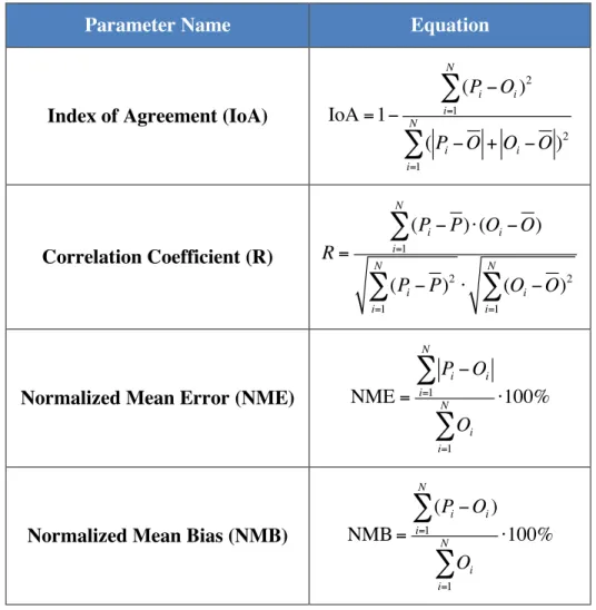
Several statistical parameters are calculated for performance evaluations, according to the recommendations from the EPA’s air quality modeling guidance [16]. Useful metrics that other studies have used for performance evaluations include the following: index of agreement (IoA), correlation coefficient (R), normalized mean error (NME), and normalized mean bias (NMB). The equations used to calculate these parameters are provided in Table 2-1.
Parameter Name Equation
Index of Agreement (IoA) IoA = 1−
(Pi− Oi) 2 i=1 N
∑
( Pi− O + Oi− O ) 2 i=1 N∑
Correlation Coefficient (R) R = (Pi− P)⋅ (Oi− O) i=1 N∑
(Pi− P) 2 i=1 N∑
⋅ (Oi− O) 2 i=1 N∑
Normalized Mean Error (NME) NME =
Pi− Oi i=1 N
∑
Oi i=1 N∑
⋅100%Normalized Mean Bias (NMB) NMB =
(Pi− Oi) i=1 N
∑
Oi i=1 N∑
⋅100%IoA is a parameter developed by Willmott [32] in 1981, and serves to be a standardized measure of the degree of model prediction error. The value of IoA varies between 0 and 1, where a value of 1 indicates a perfect match and a value of 0 indicates no agreement. Correlation coefficient is another metric used to quantify the strength of model prediction. The R-value varies between -1 and +1, where a value of 1 indicates a strong positive correlation and a value of -1 means a strong negative correlation. For model prediction, a value close to +1 would indicate good performance, since a perfect match between the observation and the model would mean a positive correlation.
NME is a metric used to measure the overall error of the modeling system. NME is normalized by the mean of the observation at the end, which allows a relative comparison without considering the actual magnitude of the measurements. NMB is similar to NME; the only difference is that for NMB calculation, the absolute values are not taken, allowing for a metric for quantifying the model bias.
According to the EPA [16], the recommended practice for performance evaluation of PM2.5 is
comparing the obtained results against similar modeling exercises to ensure that the model performance approximates the quality of other applications. Therefore, statistical parameters described above are compared against the same parameters obtained from previous modeling studies that focused on the regional-scale air quality modeling in Asia; the results of this comparison are presented in the subsequent sections.
2.4.2 Meteorology
For the performance evaluation of the meteorological model, the Global and U.S. Integrated Surface Hourly observation data from the National Climatic Data Center is used [33]. From this dataset, the observation data from 381 stations in China are retrieved and used. For this study, performance evaluation was conducted for the hourly values of temperature at 2m (T2) and wind speed at 10m (WSPD10).
Tables 2-2 and 2-3 show the statistical parameters for T2 and WSPD10, respectively, obtained from this study and the same parameters from Zhang et al. [18], Wang et al. [21], and Kwok et al.
[20]. Both Zhang et al. and Kwok et al. performed four 1-month simulations, for each of the four seasons of the year; therefore, in order to make a relevant comparison to this study’s one-year simulation that takes into account all four seasons, the values listed on these tables are seasonal average values from the four months. Wang et al. only performed a single 1-month simulation for October 2004; although not a fair comparison, the values are listed nonetheless for completeness of comparisons to other studies.
IoA R NME (%) NMB (%)
This study (2006) 0.96 0.93 26.6 -9.4
Zhang (2008) N/A 0.8 26.3 -12.0
Wang (10/2004) 0.97 N/A N/A N/A
Table 2-2: Statistical parameters obtained for temperature at 2m (T2)
IoA R NME (%) NMB (%)
This study (2006) 0.61 0.43 87.6 57.8
Zhang (2008) N/A 0.43 81.5 58.0
Wang (10/2004) 0.79 N/A N/A N/A
Kwok (2004) 0.79 0.66 35.5 -2.7
Table 2-3: Statistical parameters obtained for wind speed at 10m (WSPD10)
Observing the results from Table 2-2, it is shown that this study’s performance is on par with, or better than other studies’ prediction of T2. However, for WSPD10, this study performs on par with Zhang et al., but significantly worse compared to Wang et al. and Kwok et al. This difference in performance may be attributed to the two studies’ use of locally-available fine-resolution surface wind data used for “grid-nudging,” which matches the model output to be closer to observational data provided for the nudging process.
For a graphic representation of relative performance, a “soccer goal plot” is generated. Soccer goal plots are used in the Atmospheric Model Evaluation Tool (AMET) [34]—software designed to assist in the analysis and evaluation of meteorological and air quality models—to illustrate model performance in terms of normalized mean bias (NMB) and normalized mean error (NME).
As seen in Figure 2-5, this plot presents NMB on its x-axis and NME on its y-axis; a point far away from the origin represents large values of NMB and/or NME. Points on the right-side of the y-axis represents models with positive bias; this means that model prediction is generally greater in magnitude compared to the observations.
Figure 2-4: Soccer goal plot of meteorology model performance evaluation
The NMB and NME values from Table 2-2 and 2-3 are plotted in Figure 2-4. Again, this figure illustrates that this model’s performance is comparative to other studies’ for T2, as the circular markers are concentrated near the top edge of the 25%-soccer goal. However, the fact that they lie on the left side of the y-axis illustrates that the models generally underpredict T2. For WSPD10, there are two clusters of rectangular markers. One cluster lies near the y-axis, at about 40% NME; another cluster lies around 75% NMB and NME. The first cluster represents the studies that did not use grid-nudging, and the second cluster represents studies with grid-nudging that resulted in a better performance.
From the performance evaluation of meteorology, it is noticeable that there’s a large overprediction of wind speed throughout the modeling domain. This overprediction in wind speed is likely to affect CTM performance. The next section looks at the performance evaluation of air quality. −1000 −50 0 50 100 20 40 60 80 100 120 Meteorology
Normalized Mean Bias (%)
Normalized Mean Error (%)
T2 − this thesis T2 − Zhang
WSPD10 − this thesis WSPD10 − Zhang WSPD10 − Kwok
2.4.3 Air Quality
For the performance evaluation of the air quality model, hourly observation data from three different datasets all over Asia are used [56, 94, 95]. From these datasets, hourly observation data from 66 stations are used to compare the modeled and observed concentrations of O3, PM2.5
and PM10. Following the steps of meteorology performance evaluation, the air quality model
performance evaluation results of this thesis are compared to those of other studies.
In addition to Kwok et al. [20] and Wang et al. [21], the results of Liu et al. [17] are used for comparison. Similar to other studies, Liu et al. performs four 1-month simulations to account for the seasonal variations. Tables 2-4, 2-5, and 2-6 display the statistical parameters obtained from this thesis, and the same parameters from similar scale studies used for comparison.
IoA R NME (%) NMB (%)
This study (2006) 0.68 0.56 53.20 4.12
Kwok (2004) 0.64 N/A 76.33 45.68
Liu (2008) N/A 0.58 22.13 8.50
Wang (10/2004) N/A 0.73 37.10 -5.40
Table 2-4: Statistical parameters obtained for O3 concentration at ground
IoA R NME (%) NMB (%)
This study (2006) 0.42 0.16 84.20 -13.41
Kwok (2004) 0.53 N/A 52.15 -42.73
Table 2-5: Statistical parameters obtained for PM2.5 concentration at ground
IoA R NME (%) NMB (%)
This study (2006) 0.43 0.14 70.69 -44.92
Kwok (2004) 0.51 N/A 50.30 -41.00
Liu (2008) N/A 0.30 54.38 -43.15
Table 2-6: Statistical parameters obtained for PM10 concentration at ground
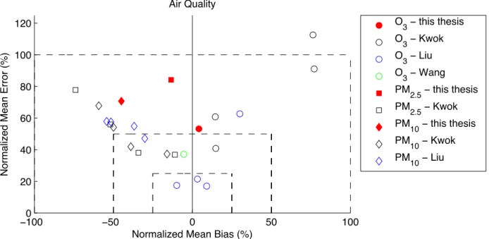
The same statistical parameters are also displayed, using a soccer goal plot, in Figure 2-5, in order to visualize the comparison between this thesis work and other studies.
Figure 2-5: Soccer goal of air quality model performance evaluation
From observing Tables 2-4 to 2-6 and Figure 2-5, this model’s performance is comparative to other studies’ for O3 concentration; however, its performance for PM species is not as
competitive. This pattern can be attributed to the relative performance of the meteorological model used in this study. From Section 2.4.2, it was found that this study overpredicts wind speed compared to the studies that used nudging. Kwok et al. and Liu et al. both used grid-nudging for their meteorological modeling and achieved a better performance in predicting wind speed. Thus, this overprediction of wind—compared to other studies—may be a contributor to the higher negative biases observed for PM concentration prediction. The impact of this negative bias on the prediction of aviation-attributable PM2.5 is uncertain, and will remain as a limitation
of this thesis work.
−1000 −50 0 50 100 20 40 60 80 100 120 Air Quality
Normalized Mean Bias (%)
Normalized Mean Error (%)
O 3 − this thesis O 3 − Kwok O 3 − Liu O 3 − Wang PM 2.5 − this thesis PM 2.5 − Kwok PM 10 − this thesis PM 10 − Kwok PM 10 − Liu
3 Background Emissions
A background emissions (non-aviation anthropogenic emissions) dataset, in conjunction with the aviation emissions dataset, is essential to quantifying the air quality impacts of aviation, because it sets the ambient conditions in which aviation emissions enter to go through complex physicochemical processes and form secondary PM. For atmospheric modeling purposes, utilizing a set of emission inputs that reflects the spatial and temporal emission profiles is necessary in achieving agreement between the model and observation concentrations of pollutants. Global-scale emissions inventories, such as Emissions Database for Global Atmospheric Research (EDGAR) [35] and Global Emissions Initiative (GEIA) [36] are utilized in global-scale CTMs.
In comparison to North America and Europe, there are relatively few Asian inventories of anthropogenic emissions available. The development of Asian emissions inventories began with Kato and Akimoto [38] and Akimoto and Narita [39], which reported SO2 and NOX emissions in
the 1990s. More recently, emissions inventories with a more complete set of air pollutant species were developed for Asia; Streets et al. [40] developed of a recent-year emissions inventory in 2003, followed by its successor, Zhang et al. [41] in 2009. Ohara et al. [42] took a step further to generate Asian anthropogenic emissions for the period 1980-2020, including future year background emissions estimates.
For this thesis, a combination of four emissions inventories—including two regional-scale Asian emissions inventories and two fine-resolution global-scale inventories—are processed to generate the CMAQ-ready background emission files. This chapter discusses the details of the four inventories, the emissions file generation methodology, and the uncertainty of the emissions.
3.1 Emissions Inventories
This section describes the four anthropogenic emissions inventories used for this thesis work. The majority of the inland emissions species comes from Streets et al. [40] and Zhang et al. [41]. A fine-resolution global emissions inventory from PBL Netherlands Environmental Assessment
Agency [43] is utilized for NH3. Lastly, shipping emissions inventory developed by Corbett et al.
[44] is used to capture the shipping emission profiles for the Asian domain.
3.1.1 TRACE-P Emissions
In 2003, Streets et al. [40] developed an emissions inventory for year 2000 that includes SOX,
NOX, CO, non-methane volatile organic compounds (NMVOC), black carbon (BC), organic
carbon (OC), NH3, and CH4. This inventory was developed to contribute to the NASA TRACE-P
(Transport and Chemical Evolution over the Pacific) Mission [45] and ACE-Asia (Asian Pacific Regional Aerosol Characterization Experiment) [46]. The domain of this dataset stretches from Pakistan in the West to Japan in the East, and from Indonesia in the South to Mongolia in the North; a map of this domain is presented in the next section, as Zhang et al. [41] is developed for the same domain.
Figure 3-1: Black carbon emissions from TRACE-P large point source locations
There are two components to this emissions dataset: gridded emissions and point-source emissions. Gridded emissions for this inventory has a 1° × 1° horizontal grid resolution; this component is disregarded for this thesis, because a more up-to-date and a finer-resolution set of gridded emissions from Zhang et al. [41], described in the following section. However, this
dataset is needed to obtain the most up-to-date large point source emissions data, which takes into account power plants and some large iron and steel plants included for CO emissions. The locations of these large point sources are determined from the RAINS-Asia (Regional Air Pollution Information and Simulation Asia) [46] and the GEIA inventory [36]. Figure 3-1 presents the locations and the amount of emitted pollutants (black carbon in this case) for 115 large point sources. Other species that are available from this dataset are CO, NMVOC, NOX,
OC, and SO2. From here on, the point-source emissions dataset obtained from Streets et al. [38]
will be referred to as TRACE-P emissions.
3.1.2 INTEX-B Emissions
Zhang et al. [41] presents a new inventory of air pollutant emissions in Asia in the year 2006, following the steps of its predecessor, TRACE-P emissions. This dataset was developed to support the Intercontinental Chemical Transport Experiment-Phase B (INTEX-B) conducted by the National Aeronautics and Space Administration (NASA). Thus, from here on, this dataset will be referred to as INTEX-B emissions.
INTEX-B emissions include particulate matter with diameters less than or equal to 10μm (PM10)
and particulate matter with diameters less than or equal to 2.5μm (PM2.5), which TRACE-P
emissions did not address. Also, the emissions numbers were updated from year 2000 to 2006, since a rapid growth of the economy and energy use in China significantly changed the amount of emitted pollutants; emissions from China are emphasized in INTEX-B, because they represent a significant fraction (between 42% and 66%) of the emissions in Asia. Growth of anthropogenic emissions in China is shown in Table 3-1; a more comprehensive comparison is presented in [41].
SOX NOX CO NMVOC PM10 PM2.5 BC OC
Growth 36% 55% 18% 29% 13% 14% 14% 14%
Table 3-1: Percentage growth of anthropogenic emissions (annual) in China from 2001 to 2006
The spatial domain of this dataset, which is identical to the domain covered by TRACE-P, is illustrated in Figure 3-2. This domain is covered by 0.5° × 0.5° horizontal grids, which is an improvement from TRACE-P’s 1° × 1° resolution.
Figure 3-2: Definition of the inventory domain (for TRACE-P and INTEX-B)
INTEX-B dataset presents an annual sum of the anthropogenic species (SO2, NOX, CO, NMVOC,
PM10, PM2.5, BC and OC) from four different source categories: power generation, industrial
production, residential combustion, and transportation (gasoline and diesel vehicles). A further discussion on the emissions from different source categories is presented in Section 3.2.5.
3.1.3 NH3 (Ammonia) Emissions
Ammonia is an important atmospheric pollutant with a wide variety of impacts, which includes its role in secondary PM formation. Major sources of ammonia emission include livestock production and fertilizer use; large portions of India and China emit a significant amount ammonia from these sources. Thus, an accurate representation of NH3 emissions in Asia is
needed for this thesis work, in order for the model to capture the formation of secondary aerosols in the atmosphere.
Ammonia emissions data is included in the TRACE-P inventory; however, a finer-resolution global emissions inventory is available from PBL (Planbureau voor de Leefomgeving) Netherlands Environmental Assessment Agency [43]. This dataset updates its predecessor [47]
with data for the year 2000 and significantly improves the horizontal grid resolution from 1° × 1° to 5min × 5min. Any reference to ammonia emissions from here on will be directed at this dataset.
The updates in the INTEX-B inventory indicate a significant growth in the amount of pollutants emitted from anthropogenic sources from 2000 to 2006. However, ammonia is not one of the species that were updated from the TRACE-P inventory; Zhang et al. [41] indicates that the amount of NH3 has not changed significantly since 2000, unlike other species that required
updates. This insignificant change in ammonia emissions from 2000 to 2006 is also confirmed by Ohara et al. [42].
3.1.4 Shipping Emissions
Aviation-attributable health impacts are calculated by observing the changes in surface-level PM2.5 concentrations and the population that are affected by the change. This method suggests
that the pollutant concentrations of grid cells directly above the oceans can be safely disregarded for health impacts calculations. However, emissions that occur over the water (i.e. shipping emissions) should not be ignored; pollutants emitted over the ocean can move into the dry land via transport mechanisms. Studies have shown that ships make a non-negligible contribution to air quality and human health [48-50].
In order to account for shipping emissions, a global ship emissions inventory developed by Wang et al. [44] is utilized for this thesis work. This inventory has 0.1° × 0.1° grid resolution, and includes monthly emission sums of SO2, NOX, CO, BC, NMVOC, and PM2.5; this inventory
updates emission values based on 2001 data with 2008 to 2010 estimates. This dataset, from here on, will be referred to as shipping emissions.
Figure 3-3 shows annual sum NOX emissions from the shipping emissions inventory. The plot
clearly displays the major shipping trade routes across the oceans. A portion of this global dataset that is within the CMAQ domain is utilized for this thesis work.
A summary of the four datasets described in the previous sections is presented in Table 3-2.
Inventory Sectors Source Type Resolution Species
Streets et al. • Power Generation Point N/A BC, OC, NOX,
SO2, CO, NMVOC Zhang et al. • Industrial • Transportation • Residential • Power Generation Gridded 0.5° × 0.5° BC, OC, NOX, SO2, PM10, PM2.5, CO, NMVOC
Beusen et al. N/A Gridded 5min × 5min NH3
Wang et al. • Shipping Gridded 0.1° × 0.1° BC, NOX, SO2,
PM2.5, CO, NMVOC
Table 3-2: A summary of the four emissions inventories used in this thesis
3.2 Methodology
As described in the previous section, four different emissions datasets are chosen for this study in order to ensure the highest resolution data available for the emissions species of interest. Combining four different inventories, however, adds difficulties in generating CMAQ-ready emissions files; the inventories vary in resolution, temporal scale, pollutant species definitions, and units used. Thus, a set of MATLAB codes were written to process and generate emissions files. This section describes the processes that were taken to generate emissions files for CMAQ.
3.2.1 Horizontal Allocation
The four datasets only define the locations of emission sources in the horizontal domain in their corresponding spatial resolutions. Therefore, the initial step taken to combine the four emissions inventories is horizontal allocation into the CMAQ modeling domain, which—as described in Chapter 2—has 164 rows and 193 columns of 50km × 50km horizontal grids.
The TRACE-P inventory has exact locations of the large point sources; with this information, the emissions are assigned to the CMAQ grids that contain the locations of the point sources. Ammonia emissions and shipping emissions are both gridded and have finer grid resolution compared to the CMAQ grids (approximately 1/6 to 1/5 of the CMAQ grid per dimension). Therefore, the grid centers of the two inventories are observed, and the corresponding emissions are assigned to the CMAQ grids that contain the inventory grid centers. Figure 3-4 illustrates the results of horizontally allocated ammonia emissions.
In order to ensure mass conservation, the emissions sum within the CMAQ domain is calculated for both raw and allocated data. The sums are consistent, as shown on the title lines of Figure 3-4. The spatial patterns of the emissions also remain consistent.
A similar process is applied to the INTEX-B inventory; however, because the grid resolution of this inventory (approximately 55km per dimension) is comparable to the CMAQ grid resolution, an extra step is required beforehand. Each INTEX-B grid is divided equally into 81 squares, along with the corresponding emission values. Then the divided INTEX-B emissions are assigned to the CMAQ grids. The result of this allocation for NOX emissions from INTEX-B is
shown in Figure 3-5. Once again, the spatial pattern of the emissions is approximately consistent; the emission sums also equal to each other.
The horizontal allocation process appropriately assigns all the monthly- (shipping) and annually- (INTEX-B, TRACE-P, and ammonia) summed emissions into the 2-D space defined during the model setup. The next section adds another dimension to the emissions profile by assigning the horizontally allocated emissions into a 3-D space.
Figure 3-4: Ammonia emissions before (top) and after (bottom) horizontal allocation
Figure 3-5: INTEX-B NOX emissions before (top)
3.2.2 Vertical Layer Assignment
Anthropogenic emissions such as residential and transportation emissions are emitted near the ground, which can be assigned to the ground-level vertical layer in the modeling domain. However, power plants and large industrial factories emit their by-product pollutants at the top of smokestacks that are designed to alleviate the impact of emitted pollutants to the surrounding region. The effective stack height is not only affected by the physical height of the smokestacks, but also is affected by buoyancy and initial momentum. As a result, large point source emissions must be properly assigned to the appropriate higher vertical layers.
From the horizontal allocation process of the TRACE-P inventory, the amount of pollutants (BC, OC, NOX, SO2, CO, NMVOC) emitted from 115 large point sources is assigned to the
appropriate CMAQ horizontal grids. However, the gridded emissions data from the INTEX-B inventory also contains up-to-date estimates of power generation emissions of the corresponding species. Therefore, a straightforward addition of the two datasets results in a double counting of power generation emissions. In order to address this issue, the CMAQ grids that contain 115 large point source locations receive special treatment.
The amount of power generation emissions from INTEX-B is compared to the amount of TRACE-P emissions for each power generation grid. If the INTEX-B emissions value is larger than the TRACE-P emissions value, the difference between the two is assigned to the ground-level vertical layer; the TRACE-P value is then assigned to an upper vertical layer using plume-rise calculations described later in this section. If the INTEX-B emissions value is smaller than the TRACE-P emissions value, then only the INTEX-B value is used and assigned to an upper vertical layer; no power generation emission is assigned to the ground level.
The methodology described above is used to determine the amount of power generation emissions to be assigned to upper vertical layers; however, the vertical location of this emission must be determined using plume rise calculations. The Sparse Matrix Operator Kernel Emissions (SMOKE) model [27], an emissions processing software widely utilized for the U.S. domain, performs plume rise calculations using the following methodology described in Equations (3.1-3.3); a detailed description of this methodology can also be found in [7].
Effective stack height ℎ = ℎ!+ Δℎ (3.1) Plume rise Δℎ = 21.4!×!! !.!"/!! !, ! < 55 38.7!×!!!.!"/!! !, ! ≥ 55 (3.2)
Buoyancy flux parameter ! = !0.25!!!!! !! − !! /!!! (3.3)
Nomenclature for Equations (3.1-3.3):
Ua = ambient velocity at stack height, m/s Vs = stack exit velocity, m/s
g = gravitational acceleration, 9.807 m/s2 Ts = stack exit temperature at h, K
d = stack inner diameter, m!! Ta = ambient temperature at h, K
Plant Unit h (m) d (m) Ts (K) Vs (m/s) Jingneng 4 210 7 / 4 323 22.4 Datang 8 120 6 353 10.2 Huaneng 4 238 6 323 22.0 Guohua 4 100 / 240 6.2 / 3.8 373 18.8 Jingfeng 2 150 3.7 338 19.6 Huadian 4 165 / 70 4.5 / 4 331 / 387 26.5 / 7.3 Taiyanggong 2 70 4 377 23.2 Caoqio 2 70 4 377 13.2
Table 3-3: Unit and stack parameters of power plants in Beijing [51]
From the tip of smokestacks, waste gases are usually emitted at temperatures above that of the ambient air and are emitted with non-negligible initial momentum. These properties of waste gases, in addition to the physical properties of the smokestacks and the ambient conditions of meteorology, can be used to calculate the effective stack height (h)—the sum of the actual stack height (hs) and the plume rise (Δh).
Meteorological variables (Ua and Ta) are obtained from the meteorological fields from WRF
simulations described in Section 2.3.1. Due to a lack of available information on the smokestack parameters of the large point sources, average values of the available information from Table 3-3 (adapted from Hao et al. [51]) are used.
The above methodology is used for species that are included in the TRACE-P inventory; however, power generation emissions for PM10 and PM2.5 are only available in gridded form of
INTEX-B inventory. A study by Wang et al. [52] derives the vertical profiles for East Asia based on the U.S. EPA NEI99 to allocate power generation emissions to different vertical layers. This study assigns the following percentages of PM2.5 (and PM10) emissions into different vertical
layers as follows: 5% (5%) below 76m above ground; 45% (55%) between 76m and 153m above ground; 25% (20%) between 153m and 308m above ground; 20% (15%) between 308m and 547m above ground; and 5% (5%) between 547m and 871m above ground. This profile is adapted to assign PM emissions (excluding BC and OC) into the vertical layers of this model setup. BC and OC emissions are assigned to vertical layers using plume rise calculations, since they are included in the TRACE-P inventory.
3.2.3 Temporal Variation
Another dimension considered for background emissions processing is time, as CMAQ-ready emissions input files are required to have one-hour time steps. Because the emissions input require such a fine temporal resolution, it is important to consider temporal variations in emissions for different time scales (from seasonal to diurnal) as well as different sectors. However, many of the temporal profiles required to process Asian emissions are not available. Thus, for this thesis, as much of the available temporal profile information for the Asian domain are utilized; temporal profiles that are not available for the Asian domain are adapted from other regions (i.e. Europe or the U.S.) or kept invariant.
Various temporal profiles that take into account the seasonal variability of different emission sectors are utilized for this study. Pollutant species that are included in the INTEX-B inventory are considered combustion-related, and the corresponding monthly fractions for the residential, power generation, and industrial sector emissions are adapted from Streets et al. [40] and Zhang et al. [53].
Monthly variation for the residential sector is estimated for China by examining the monthly mean temperatures of each province, assuming a dependence of stove operation on provincial monthly mean temperatures. Power generation and industrial sector monthly profiles are
obtained using monthly data on power generation, cement production, and industrial GDP for the period 1995-2004 [54]. The transportation sector lacks a monthly profile for the Asian domain. With this absence of relevant information, other studies have used European monthly profiles and the use was shown to improve air quality simulations over Nanjing [55] and also the entire Asian domain [52]; therefore, an available profile for the European domain from Olivier et al. [57] is used for this thesis work, although the applicability of the European emissions profile to Asia is uncertain.
Ammonia, not considered to be a combustion-related species (except as relates to after-treatment technologies), adapts a different monthly profile presented in Streets et al. [40]. This profile is constructed considering a temperature dependence of emissions of ammonia from animal waste and fertilizer application for agricultural purposes. Beusen et al. [43] reports shipping emissions monthly, so the seasonal variation is already taken into account.
Figure 3-6 displays the six monthly profiles described in this section. As expected, the residential sector puts higher fraction of the annual total to the winter, as lower outdoor temperatures in the winter is expected to increase residential heating. Also, ammonia emissions peak in late spring and early summer, as the profile is developed based on agricultural activities such as animal waste and fertilizer application, which is most active during those months.
Figure 3-6: Monthly profiles used in this thesis
Jan Feb Mar Apr May Jun Jul Aug Sep Oct Nov Dec
0 0.02 0.04 0.06 0.08 0.1 0.12 0.14 0.16 0.18 0.2 Month
Fraction of annual emissions
Industry Power Residential Transportation Ammonia Shipping