Adjoint Sensitivity Analysis of the
Intercontinental Impacts of Aviation Emissions on
Air Quality and Health
by
Jamin Koo
B.S., University of Illinois at Urbana-Champaign (2009)
Submitted to the School of Engineering
in partial fulfillment of the requirements for the degree of
Master of Science in Computation for Design and Optimization
at the
MASSACHUSETTS INSTITUTE OF TECHNOLOGY
September 2011
c
Massachusetts Institute of Technology 2011. All rights reserved.
Author . . . .
School of Engineering
August 4, 2011
Certified by . . . .
Qiqi Wang
Assistant Professor of Aeronautics and Astronautics
Thesis Supervisor
Accepted by . . . .
Nicolas Hadjiconstantinou
Associate Professor of Mechanical Engineering
Director, Computation for Design and Optimization Program
Adjoint Sensitivity Analysis of the Intercontinental Impacts
of Aviation Emissions on Air Quality and Health
by
Jamin Koo
Submitted to the School of Engineering on August 4, 2011, in partial fulfillment of the
requirements for the degree of
Master of Science in Computation for Design and Optimization
Abstract
Over 10,000 premature mortalities per year globally are attributed to the exposure to particulate matter caused by aircraft emissions. Unlike previous studies that fo-cus on the regional impacts from the aircraft emissions below 3,000 feet, this thesis studies the impact from emissions at all altitudes and across continents on increasing particulates in a receptor region, thereby increasing exposure. In addition to these intercontinental impacts, the thesis analyzes the temporal variations of sensitivities of the air quality and health, the proportion of the impacts attributable to different emission species, and the background emissions’ influence on the impact of aircraft emissions.
To quantify the impacts of aircraft emissions at various locations and times, this study uses the adjoint model of GEOS-Chem, a chemical transport model. The adjoint method efficiently computes sensitivities of a few objective functions, such as aggregated PM concentration and human exposure to PM concentration, with respect to many input parameters, i.e. emissions at different locations and times.
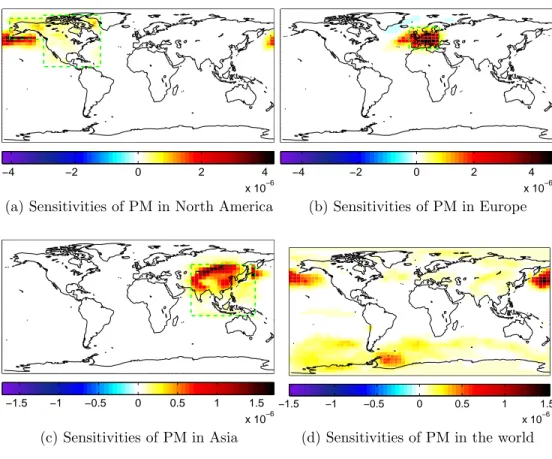
Whereas emissions below 3,000 feet have mostly local impacts, cruise emissions from North America impair the air quality in Europe and Asia, and European cruise emissions affect Asia. Due to emissions entering Asia, the premature mortalities in Asia were approximately two to three times larger than the global mortalities caused by the Asian emissions. In contrast, North America observed only about one-ninth of the global premature mortalities caused by North American emissions because emissions get carried out of the region. This thesis calculates that most of the premature mortalities occured in Europe and Asia in 2006.
Sensitivities to emissions also have seasonal and diurnal cycles. For example, ground level NOX emissions in the evening contribute to 50% more surface PM
for-mation than the same emissions in the morning, and cruise level NOX emissions in
early winter cause six times more PM concentration increase than the same emis-sions in spring. Aircraft NOX emissions cause 78% of PM from aviation emissions,
and given the population exposure to PM concentration increase, NOX contributes
that increases in background emissions of ammonia increase the impact of aircraft emissions on the air quality and increases in background NOX emissions decrease the
impact.
These results show the effectiveness of the adjoint model for analyzing the long-term sensitivities. Some of the analyses presented are practically only possible with the adjoint method. By regulating emissions at high sensitivities in time and region, calculated by the adjoint model, governments can design effective pollutant reduction policies.
Thesis Supervisor: Qiqi Wang
Acknowledgments
First I would like to thank my advisor, Professor Qiqi Wang, for his great support. I am very lucky to become the first student of Professor Wang, who is patient and understanding, while providing a great research guidance with enthusiasm. Professor Steven Barrett deserves sincere appreciation for his great explaination of atmospheric science and thorough comments throughout the course of this research. I cannot think of anyone else who is willing to and is capable of examining my writing in such detail. I am also priviledged to work under the supervision of Professor Ian A. Waitz, the dean of engineering at MIT. Knowing his support on this project and having conversations with him fostered inspirations and confidences; in one sentence, he is an extraordinary advisor. I also thank Chris Sequeira for his support; he has been very attentive to my research and its progress, providing valuable feedbacks in a timely manner. Professor Daven Henze of the University of Colorado at Boulder is definitely at the top of my list to appreciate. There were about four hundered e-mails sent back and forth between Daven and me, while he helped me tremendously with running GEOS-Chem Adjoint and I bugged him with various bug reports. I am also thankful to Laura Koller, an academic administrator for Computation for Design and Optimization, for making my educational experience trouble-free.
Next round of my acknowledgement goes to researchers and students in PART-NER. I thank Akshay Ashok, who is the most deterministic person I have ever met, for sitting next to me and answering my never-ending questions related to this research with 0% uncertainty and Rhea Liem, who is a complement of Akshay in a probabilis-tic sense(Rhea=Akshayc), for bringing exciting and fonding moments to the lab at a random sequence. I also thank Philip Wolfe and Alex Nakahara for bearing with my constant noisy chat with Akshay, while educating me with obscure facts that can only be learned through extensive reading or participating in trivias. I also thank Steve Yim, Christoph Wollersheim, Hossam El-Asrag, Alex Mozdzanowska, Jim Hileman, Mina Jun, Fabio Caiazzo, Chris Gilmore, Kevin Lee, Gideon Lee, Sergio Amaral and everyone else in the lab for making PARTNER a great, lively, loving place. It would
also be unwise of me to forget thanking the unknown hacker who hacked our linux clusters from Netherlands, giving me frustration, anxiety, and more work in addition to having me delay my graduation date.
My final and sincere acknowledgement goes to the three greatest teachers of Maum Meditation, who have continuously provided me with care and love in addition to helping me become who I am now and providing me a lifetime guidance.
Without the help of everyone around me, not limited to the people I mentioned above, my experience at MIT and growth as a researcher would have not been fun, fruitful, and rewarding to this extent.
Contents
1 Introduction 21
1.1 Aviation Activities and Policies . . . 21
1.2 Air Pollution and Health Impacts . . . 23
1.3 Motivation for Adjoint Sensitivity Analysis . . . 25
1.4 Thesis Organization . . . 26
2 The Adjoint Method 29 2.1 Advantages of Adjoint Analysis . . . 31
2.2 GEOS-Chem, a Chemical Transport Model . . . 32
2.2.1 GEOS-Chem and GEOS-Chem Adjoint . . . 33
2.2.2 Aircraft Emissions Inventory . . . 35
2.2.3 Improvement to GEOS-Chem Adjoint . . . 36
2.2.4 Verification of the Adjoint Model in GEOS-Chem . . . 38
3 Sensitivity Results 43 3.1 Definition of Sensitivities . . . 43
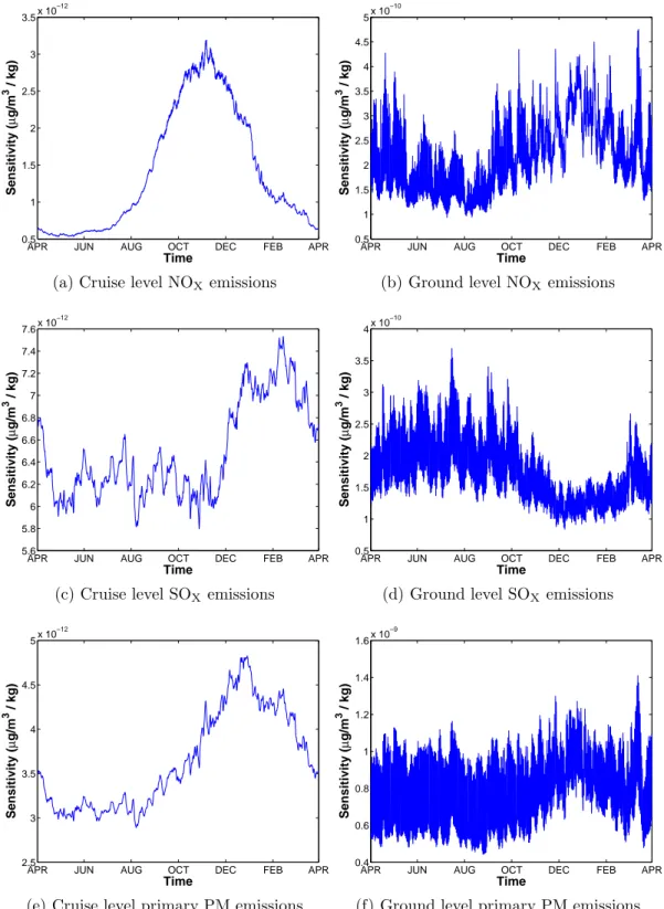
3.1.1 Interpreting Sensitivity Plots in this Thesis . . . 44
3.2 Spin-Up Period . . . 45
3.3 Premature Mortality Calculation . . . 48
3.4 Regional PM Exposure due to Intercontinental Effects . . . 50
3.4.1 Landing and Take-off Emissions . . . 50
3.4.2 Cruise Emissions . . . 54
3.5 Effect of Seasons and Times of Day . . . 59
3.5.1 Diurnal Cycle . . . 59
3.5.2 Seasonal Cycle . . . 61
3.6 Sensitivities of Each PM Species to Aircraft Emissions . . . 63
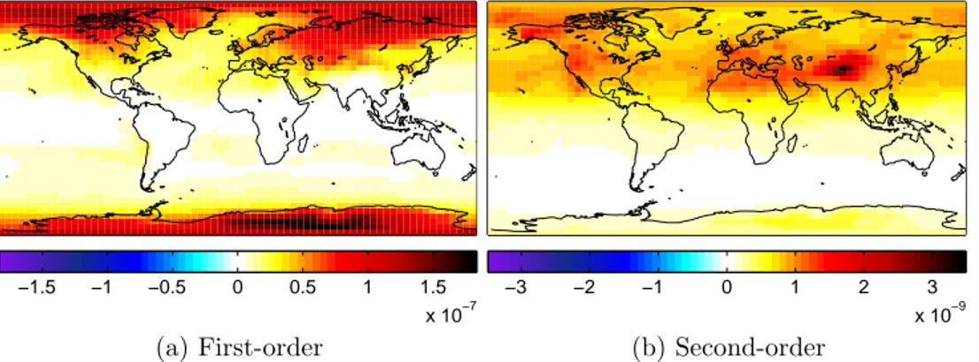
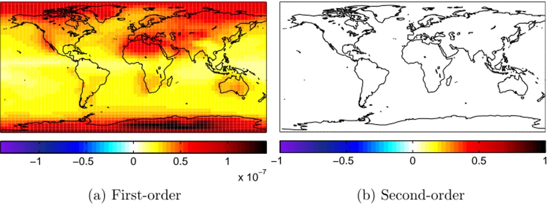
3.7 Second-order Sensitivities . . . 65
4 Conclusions and Future Work 69 4.1 Conclusions . . . 69
4.1.1 Intercontinental Impacts . . . 70
4.1.2 Temporal Variation in Sensitivities . . . 70
4.1.3 Proportion of the Impacts of Different Aircraft Emissions Species 70 4.1.4 Second-order Sensitivities . . . 71
4.2 Future Work . . . 71
4.2.1 Limitations and Future Improvements . . . 71
4.2.2 Potential Topics for Future Work . . . 72
4.2.3 Policy Implications . . . 73
A Conversion between Discrete and Continuous Adjoint Variables 81 B Sensitivity Plots 85 B.1 Sensitivities of Surface PM Concentration . . . 85
B.1.1 Sensitivities of Surface PM concentration in the US to Aircraft Emissions . . . 85
B.1.2 Sensitivities of Surface PM concentration in North America to Aircraft Emissions . . . 89
B.1.3 Sensitivities of Surface PM concentration in Europe to Aircraft Emissions . . . 92
B.1.4 Sensitivities of Surface PM concentration in Asia to Aircraft Emissions . . . 95
B.1.5 Sensitivities of Surface PM concentration in the World to Air-craft Emissions . . . 98
B.2 Sensitivities of Population Exposure to PM . . . 101 B.2.1 Sensitivities of Population Exposure to PM in the US to
Air-craft Emissions . . . 101 B.2.2 Sensitivities of Population Exposure to PM in North America
to Aircraft Emissions . . . 104 B.2.3 Sensitivities of Population Exposure to PM in Europe to
Air-craft Emissions . . . 107 B.2.4 Sensitivities of Population Exposure to PM in Asia to Aircraft
Emissions . . . 110 B.2.5 Sensitivities of Population Exposure to PM in the World to
Aircraft Emissions . . . 113
C Second-order Sensitivity Plots 117
List of Figures
1-1 Forward and adjoint analyses . . . 26 2-1 Discrete and continuous adjoint . . . 30 2-2 Order of operations for forward method versus adjoint method . . . . 31
2-3 GEOS-Chem forward and adjoint modules . . . 34
2-4 Regions considered in this thesis . . . 35 2-5 Adjoint vs finite difference results for kg·hr of aerosol produced due to
aircraft NOX, SOX, and HC emissions . . . 39
2-6 Adjoint vs finite difference results for kg·hr of aerosol produced due to aircraft CO, BC, and OC emissions . . . 40 3-1 Sensitivities of global surface PM concentration to NOX emissions (in
µg m−3/kg hr−1) and global aircraft NO
X emission rate (in kg hr−1)
averaged over all altitudes: Inner product of two matrices gives the change in PM concentration (in µg/m3) due to aircraft NO
X emissions 45
3-2 Explanation of spin-up period . . . 46 3-3 Comparison of different spin-up periods of the sensitivities of surface
PM concentration in the US to global aircraft emissions . . . 47 3-4 Ratio of impacts in the last month captured from simulations with
different spin-up periods compared to a simulation with a six-month spin-up period . . . 48 3-5 Sensitivities of surface PM concentration (in µg/m3) in Europe with
3-6 Sensitivities of surface PM concentration in various regions with re-spect to ground level NOX emissions (in µg m−3/kg hr−1) . . . 52
3-7 Sensitivities of surface PM concentration in various regions with re-spect to cruise level NOX emissions (in µg m−3/kg hr−1) . . . 55
3-8 Sensitivities of surface PM concentration in the US due to 1kg/hr of NOX emissions (in µg m−3/kg hr−1) . . . 56
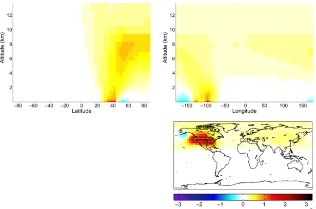
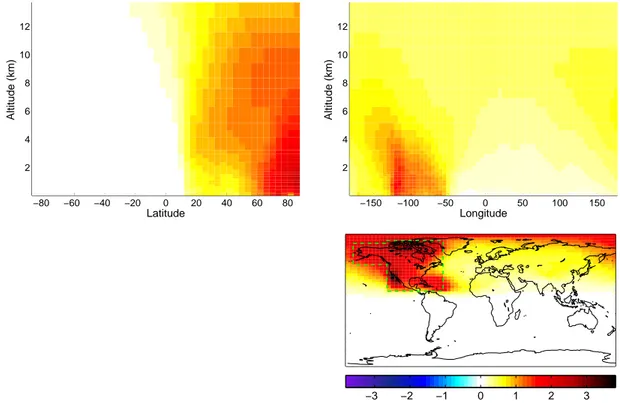
3-9 Streamline of wind and the transport of PM from aircraft emissions [1] 57 3-10 Sensitivities of global surface PM concentration averaged over 365 days
to various emissions at different local times of day for aviation . . . . 60 3-11 Sensitivities of global surface PM concentration to various emissions
at different times of year for aviation . . . 62 3-12 Change in annual average of the surface level nitrate and sulfate
con-centrations caused by aviation emissions simulated using the forward model of GEOS-Chem (in µg/m3) . . . . 65
3-13 First- and second-order sensitivities of global surface PM concentration with respect to ammonia emissions (in µg m−3/kg hr−1) . . . . 66
3-14 First- and second-order sensitivities of global surface PM concentration with respect to NOX emissions (in µg m−3/kg hr−1) . . . 66
3-15 First- and second-order sensitivities of global surface PM concentration with respect to SO2 emissions (in µg m−3/kg hr−1) . . . 67
3-16 First- and second-order sensitivities of global surface PM concentration with respect to primary PM emissions (in µg m−3/kg hr−1) . . . . 67
A-1 Resulting sensitivities from running with incorrect unit conversion . . 84 A-2 Resulting sensitivities from running with correct unit conversion . . . 84 B-1 Sensitivities of surface PM concentration in the US to NOX emissions
(in µg m−3/kg hr−1) . . . . 86
B-2 Sensitivities of surface PM concentration in the US to SOX emissions
B-3 Sensitivities of surface PM concentration in the US to HC emissions (in µg m−3/kg hr−1) . . . . 87
B-4 Sensitivities of surface PM concentration in the US to CO emissions (in µg m−3/kg hr−1) . . . . 87
B-5 Sensitivities of surface PM concentration in the US to primary PM emissions (in µg m−3/kg hr−1) . . . . 88
B-6 Sensitivities of surface PM concentration in North America to NOX
emissions (in µg m−3/kg hr−1) . . . . 89
B-7 Sensitivities of surface PM concentration in North America to SOX
emissions (in µg m−3/kg hr−1) . . . . 90
B-8 Sensitivities of surface PM concentration in North America to HC emis-sions (in µg m−3/kg hr−1) . . . . 90
B-9 Sensitivities of surface PM concentration in North America to CO emis-sions (in µg m−3/kg hr−1) . . . . 91
B-10 Sensitivities of surface PM concentration in North America to primary PM emissions (in µg m−3/kg hr−1) . . . . 91
B-11 Sensitivities of surface PM concentration in Europe to NOX emissions
(in µg m−3/kg hr−1) . . . . 92
B-12 Sensitivities of surface PM concentration in Europe to SOX emissions
(in µg m−3/kg hr−1) . . . . 93
B-13 Sensitivities of surface PM concentration in Europe to HC emissions (in µg m−3/kg hr−1) . . . . 93
B-14 Sensitivities of surface PM concentration in Europe to CO emissions (in µg m−3/kg hr−1) . . . . 94
B-15 Sensitivities of surface PM concentration in Europe to primary PM emissions (in µg m−3/kg hr−1) . . . . 94
B-16 Sensitivities of surface PM concentration in Asia to NOXemissions (in
µg m−3/kg hr−1) . . . . 95
B-17 Sensitivities of surface PM concentration in Asia to SOX emissions (in
B-18 Sensitivities of surface PM concentration in Asia to HC emissions (in µg m−3/kg hr−1) . . . . 96
B-19 Sensitivities of surface PM concentration in Asia to CO emissions (in µg m−3/kg hr−1) . . . . 97
B-20 Sensitivities of surface PM concentration in Asia to primary PM emis-sions (in µg m−3/kg hr−1) . . . . 97
B-21 Sensitivities of surface PM concentration in the world to NOXemissions
(in µg m−3/kg hr−1) . . . . 98
B-22 Sensitivities of surface PM concentration in the world to SOXemissions
(in µg m−3/kg hr−1) . . . . 99
B-23 Sensitivities of surface PM concentration in the world to HC emissions (in µg m−3/kg hr−1) . . . . 99
B-24 Sensitivities of surface PM concentration in the world to CO emissions (in µg m−3/kg hr−1) . . . 100
B-25 Sensitivities of surface PM concentration in the world to primary PM emissions (in µg m−3/kg hr−1) . . . 100
B-26 Sensitivities of population exposure to PM in the US to NOXemissions
(in ppl · µg m−3/kg hr−1) . . . 101
B-27 Sensitivities of population exposure to PM in the US to SOX emissions
(in ppl · µg m−3/kg hr−1) . . . 102
B-28 Sensitivities of population exposure to PM in the US to HC emissions (in ppl · µg m−3/kg hr−1) . . . 102
B-29 Sensitivities of population exposure to PM in the US to CO emissions (in ppl · µg m−3/kg hr−1) . . . 103
B-30 Sensitivities of population exposure to PM in the US to primary PM emissions (in ppl · µg m−3/kg hr−1) . . . 103
B-31 Sensitivities of population exposure to PM in North America to NOX
emissions (in ppl · µg m−3/kg hr−1) . . . 104
B-32 Sensitivities of population exposure to PM in North America to SOX
B-33 Sensitivities of population exposure to PM in North America to HC emissions (in ppl · µg m−3/kg hr−1) . . . 105
B-34 Sensitivities of population exposure to PM in North America to CO emissions (in ppl · µg m−3/kg hr−1) . . . 106
B-35 Sensitivities of population exposure to PM in North America to pri-mary PM emissions (in ppl · µg m−3/kg hr−1) . . . 106
B-36 Sensitivities of population exposure to PM in Europe to NOXemissions
(in ppl · µg m−3/kg hr−1) . . . 107
B-37 Sensitivities of population exposure to PM in Europe to SOXemissions
(in ppl · µg m−3/kg hr−1) . . . 108
B-38 Sensitivities of population exposure to PM in Europe to HC emissions (in ppl · µg m−3/kg hr−1) . . . 108
B-39 Sensitivities of population exposure to PM in Europe to CO emissions (in ppl · µg m−3/kg hr−1) . . . 109
B-40 Sensitivities of population exposure to PM in Europe to primary PM emissions (in ppl · µg m−3/kg hr−1) . . . 109
B-41 Sensitivities of population exposure to PM in Asia to NOX emissions
(in ppl · µg m−3/kg hr−1) . . . 110
B-42 Sensitivities of population exposure to PM in Asia to SOX emissions
(in ppl · µg m−3/kg hr−1) . . . 111
B-43 Sensitivities of population exposure to PM in Asia to HC emissions (in ppl · µg m−3/kg hr−1) . . . 111
B-44 Sensitivities of population exposure to PM in Asia to CO emissions (in ppl · µg m−3/kg hr−1) . . . 112
B-45 Sensitivities of population exposure to PM in Asia to primary PM emissions (in ppl · µg m−3/kg hr−1) . . . 112
B-46 Sensitivities of population exposure to PM in the world to NOX
emis-sions (in ppl · µg m−3/kg hr−1) . . . 113
B-47 Sensitivities of population exposure to PM in the world to SOX
B-48 Sensitivities of population exposure to PM in the world to HC emissions (in ppl · µg m−3/kg hr−1) . . . 114
B-49 Sensitivities of population exposure to PM in the world to CO emis-sions (in ppl · µg m−3/kg hr−1) . . . 115
B-50 Sensitivities of population exposure to PM in the world to primary PM emissions (in ppl · µg m−3/kg hr−1) . . . 115
C-1 First- and second-order sensitivities of global surface PM concentration with respect to NOX emissions (in µg m−3/kg hr−1) . . . 117
C-2 First- and second-order sensitivities of global surface PM concentration with respect to OX emissions (in µg m−3/kg hr−1) . . . 118
C-3 First- and second-order sensitivities of global surface PM concentration with respect to PAN emissions (in µg m−3/kg hr−1) . . . 118
C-4 First- and second-order sensitivities of global surface PM concentration with respect to CO emissions (in µg m−3/kg hr−1) . . . 118
C-5 First- and second-order sensitivities of global surface PM concentration with respect to ALK4 emissions (in µg m−3/kg hr−1) . . . 119
C-6 First- and second-order sensitivities of global surface PM concentration with respect to ISOP emissions (in µg m−3/kg hr−1) . . . 119
C-7 First- and second-order sensitivities of global surface PM concentration with respect to HNO3 emissions (in µg m−3/kg hr−1) . . . 119
C-8 First- and second-order sensitivities of global surface PM concentration with respect to H2O2 emissions (in µg m−3/kg hr−1) . . . 120
C-9 First- and second-order sensitivities of global surface PM concentration with respect to ACET emissions (in µg m−3/kg hr−1) . . . 120
C-10 First- and second-order sensitivities of global surface PM concentration with respect to MEK emissions (in µg m−3/kg hr−1) . . . 120
C-11 First- and second-order sensitivities of global surface PM concentration with respect to ALD2 emissions (in µg m−3/kg hr−1) . . . 121
C-12 First- and second-order sensitivities of global surface PM concentration with respect to RCHO emissions (in µg m−3/kg hr−1) . . . 121
C-13 First- and second-order sensitivities of global surface PM concentration with respect to MVK emissions (in µg m−3/kg hr−1) . . . 121
C-14 First- and second-order sensitivities of global surface PM concentration with respect to MACR emissions (in µg m−3/kg hr−1) . . . 122
C-15 First- and second-order sensitivities of global surface PM concentration with respect to PMN emissions (in µg m−3/kg hr−1) . . . 122
C-16 First- and second-order sensitivities of global surface PM concentration with respect to PPN emissions (in µg m−3/kg hr−1) . . . 122
C-17 First- and second-order sensitivities of global surface PM concentration with respect to R4N2 emissions (in µg m−3/kg hr−1) . . . 123
C-18 First- and second-order sensitivities of global surface PM concentration with respect to PRPE emissions (in µg m−3/kg hr−1) . . . 123
C-19 First- and second-order sensitivities of global surface PM concentration with respect to C3H8 emissions (in µg m−3/kg hr−1) . . . 123
C-20 First- and second-order sensitivities of global surface PM concentration with respect to CH2O emissions (in µg m−3/kg hr−1) . . . 124
C-21 First- and second-order sensitivities of global surface PM concentration with respect to C2H6 emissions (in µg m−3/kg hr−1) . . . 124
C-22 First- and second-order sensitivities of global surface PM concentration with respect to N2O5 emissions (in µg m−3/kg hr−1) . . . 124
C-23 First- and second-order sensitivities of global surface PM concentration with respect to HNO4 emissions (in µg m−3/kg hr−1) . . . 125
C-24 First- and second-order sensitivities of global surface PM concentration with respect to MP emissions (in µg m−3/kg hr−1) . . . 125
C-25 First- and second-order sensitivities of global surface PM concentration with respect to DMS emissions (in µg m−3/kg hr−1) . . . 125
C-26 First- and second-order sensitivities of global surface PM concentration with respect to SO2 emissions (in µg m−3/kg hr−1) . . . 126
C-27 First- and second-order sensitivities of global surface PM concentration with respect to SO4 emissions (in µg m−3/kg hr−1) . . . 126
C-28 First- and second-order sensitivities of global surface PM concentration with respect to NH3 emissions (in µg m−3/kg hr−1) . . . 126
C-29 First- and second-order sensitivities of global surface PM concentration with respect to NH4 emissions (in µg m−3/kg hr−1) . . . 127
C-30 First- and second-order sensitivities of global surface PM concentration with respect to NIT emissions (in µg m−3/kg hr−1) . . . 127
C-31 First- and second-order sensitivities of global surface PM concentration with respect to primary PM emissions (in µg m−3/kg hr−1) . . . 127
List of Tables
2.1 Coordinates of regions used in this thesis . . . 35 2.2 Yearly full flight emissions in various regions . . . 35 2.3 Percentage of LTO emissions over total aircraft emissions in the world 36 2.4 Slope of linear regression line for forward difference sensitivities versus
adjoint sensitivities . . . 41 2.5 r2 of linear regression line for forward difference sensitivities versus
adjoint sensitivities . . . 41 2.6 Comparison of forward difference and adjoint sensitivities for the
trans-port module . . . 42 3.1 Baseline incidence rates and fraction of population over the age of 30 49 3.2 Risk coefficients in the US from Pope et al. 2002 [2] and Laden et al.
2006 [3] . . . 49 3.3 Impact of LTO emissions in source regions on surface PM
concentra-tions in receptor regions (in ×10−3µg/m3) . . . . 53
3.4 Impact of LTO emissions in source regions on population exposures to PM in receptor regions (in ×106people · µg/m3) . . . . 53
3.5 Impact of LTO emissions in source regions on premature mortalities in receptor regions with the 95% confidence interval (in people) . . . 54 3.6 Impact of full flight emissions in source regions on surface PM
concen-trations in receptor regions (in ×10−3µg/m3) . . . . 56
3.7 Impact of full flight emissions in source regions on population exposures to PM in receptor regions (in ×106people · µg/m3) . . . . 57
3.8 Impact of full flight emissions in source regions on premature mortali-ties in receptor regions with the 95% confidence interval (in people) . 58 3.9 Change in each PM species concentration due to aviation emissions (in
%) . . . 64 3.10 Change in population exposure to each PM species due to aviation
emissions (in %) . . . 64 D.1 GEOS-Chem tracers . . . 129
Chapter 1
Introduction
Intercontinental transport of air pollution has been studied by various researches both using observations and numerical simulations. It is estimated that 380,000 premature mortalities per year are caused by aerosols produced and transported from other re-gions, among which 90,000 mortalities are caused by exposure to non-dust aerosols [4]. Besides aerosols, the precursors of aerosols and ozone are also transported across con-tinents, causing negative health impacts. Mortalities caused by ozone in a receptor continent can be reduced by about 20 to 50% when ozone precursor emissions are re-moved completely in other continents [5]. These researches, along with other studies on intercontinental transport of pollutants, suggest the importance of a hemispheric treaty on regulating emissions [6]. The impact from long range transport of pollu-tants is especially important considering emissions from aircraft. Aircraft emissions are unique in that they are emitted at higher altitudes, remaining in the atmosphere longer and being transported to a farther distance due to stronger winds aloft. Be-cause of the long-range transport, studying the cruise emissions’ impact on the air quality requires the intercontinental transport of pollutants.
1.1
Aviation Activities and Policies
The aviation sector is projected to grow at an annual rate of 4.8 - 5 % and will double the current aircraft activities by 2020 to 2025 [7, 8, 9]. Aviation activities are highly
correlated with economic trends and GDP. High growth rates in Asia, notably China and India, are driving the demand of the aviation industry [7]. Although current research shows that the contribution of aviation emissions to environmental damage is small, about 0.1% of anthropogenic pollution, compared to 1% of highway pollution in the U.S., it is important to control the emissions of this sector because of the rapid growth of air transportation [10].
The International Civil Aviation Organization (ICAO), an organization of the United Nation, created the Committee for Aviation Environmental Protection (CAEP) to analyze environmental policies for aviation and further establish standards for noise and emissions. Three environmental goals of ICAO [7]. are
• “to limit or reduce the number of people affected by significant aircraft noise”; • “to limit or reduce the adverse impact of aviation emissions on local air quality”; • “and to limit or reduce the impact of aviation greenhouse gas emissions on the
global climate.”
Aircraft noise is the first regulated because it is readily perceived in the vicinity of airports, first regulated by ICAO’s noise certification at an international level in 1971. In 1981, ICAO set the NOx emissions standard, which became effective in 1986, to
improve the air quality of the near-by regions of airports [7]. In addition to the local air quality, its focus expanded to the global climate impact. In addition, emissions standards have become more stringent as listed in the latest updated standards in ICAO Annex 16 - Environmental Protection, Volume II - Aircraft Engine Emissions to the Convention on International Civil Aviation [9].
Member states of ICAO, currently 183 countries, are recommended to implement ICAO Standards and Recommended Practices (SARPs). The U.S., as a member state, adopted several regulations based on updates of ICAO’s SARPs. Moreover, in the U.S. the Partnership for AiR Transportation Noise and Emissions Reduction (PART-NER), an FAA Center of Excellence, was formed to assess the impact of aviation emissions on climate change, air quality, and noise. To study the costs and benefits
of different policies for environment, the Aviation environmental Portfolio Manage-ment Tool (APMT) was developed by Federal Aviation Administration (FAA) and PARTNER and is currently being used [11, 12]. The work of this thesis will aid the tool suite development on the aspect of assessing the air quality impacts of aviation. Specifically, it will provide the spatial and temporal sensitivity matrices of air quality with respect to aviation emissions. The sensitivities quantify how emissions in differ-ent regions damage air quality to differdiffer-ent extdiffer-ents, which can assist policymakers in implementing effective emission reduction strategies.
1.2
Air Pollution and Health Impacts
The aviation policies of the US and other member nations of ICAO are in accordance with other regulations concerning air quality. The Clean Air Act of 1970 and 1977 in the U.S. authorized the Environmental Protection Agency (EPA) to regulate the national air quality using National Ambient Air Quality Standards; the EPA updated these standards on several occasions, with the last air quality standards for PM2.5 set
at the annual mean of 15.0 µg/m3 and 35 µg/m3 for 24-hour average [13, 14]. These
standards also set ozone level at 0.075 ppm for 8-hour and 0.12 ppm for 1-hour averages, as well as setting different annual means limits for nitrogen oxides, sulfur dioxides, lead, and carbon monoxide [15].
These standards were established based on research on health impacts caused by these pollutants. Many of these studies found a high correlation between long-term exposure to PM2.5 and lung cancer and cardiopulmonary disease [2, 16]. Particulate
matter is a mixture of liquid droplets and particles that can be inhaled. Among var-ious categories of PM, PM2.5, or particulate matter with diameter less than 2.5µm,
is found to be more damaging when exposed for a long term period. The Environ-mental Protection Agency (EPA) lists the health consequences: cardiovascular symp-toms, cardiac arrhythmias, heart attacks, respiratory sympsymp-toms, asthma attacks, and bronchitis that could result in increased hospital admissions, emergency room visits, absences from school or work, and restricted activity days [14].
Most of the air quality impacts caused by aviation emissions come from the for-mation of PM2.5, which can be categorized into primary PM and secondary PM [10].
Primary particulate matter is PM that is directly emitted from an engine or formed immediately after exiting an engine; this category includes non-volatile PM - assumed to be black carbon (BC), or soot - and volatile PM from sulfur and organics, or or-ganic carbon (OC). OC is formed about 30 meters behind the engine when volatile organic compounds (VOCs) are photo-oxidized and condensate to form organic car-bon [17, 18]. Secondary PM is formed through chemical reaction of its precursors with other chemical species in the atmosphere. The precursors are nitrogen oxides (NOx), sulfur dioxide (SO2), and volatile organic compounds. When NOx and SO2
are emitted, they are oxidized, becoming HNO3 and H2SO4. The oxidization
pro-cess can be achieved with OH, ozone, and H2O2, and the availability of the oxidants
determines the amount of PM formation [19]. As a neutralization process, sulfuric acid and ammonia form ammonium sulfate, (NH4)2SO4, and the remaining ammonia
reacts with nitrate to form ammonium nitrate, NH4NO3 [20]. Ammonium sulfate and
ammonium nitrate are the most important secondary PM species. Volatile organic compounds, or hydrocarbons, can also form secondary particulates. Both primary and secondary particulate matter introduced by aircraft emissions are PM2.5 [21].
In addition to the formation of particulates, aviation emissions cause the formation of ozone. The ozone production pathway due to aviation emissions is 1) volatile organic compounds and carbon monoxide emitted from aircraft are oxidized, and then 2) the resulting species react with NOx to form ozone [20]. It is understood
that exposure to ozone causes asthma, bronchitis, breathing difficulties, coughing, irritation, and permanent lung damage [15]. The health impact caused by aircraft emissions induced ozone is estimated to be about 4% to 8% of the impact from aviation induced PM2.5 [10, 22] although this proportion on the health impact does
1.3
Motivation for Adjoint Sensitivity Analysis
Most studies on aviation’s air quality impacts in the last few decades focus on aircraft’s landing and take-off (LTO) emissions, or emissions below 3,000 feet. However, a recent study by Barrett et al. [1] shows that aerosols created from aircraft emissions above 3,000 feet have global health impact of about 8,000 premature mortalities per year. Understanding that the health impact from emissions above 3,000 feet is two to four times larger than the impact from LTO emissions, this thesis focuses on how emissions in various regions, at both low and high altitudes, impact the ground level air quality, thereby causing premature mortalities.
Furthermore, emissions at different geographical locations have different influences on air quality. A study by Sequeira [23] indicates that the regional variability on the health effects of aviation emissions are large. The aviation LTO emission induced PM related mortalities in Los Angeles county are 18% of that of the US as a whole, and 43% of PM mortalities in the US occurs in ten counties with the highest PM-related mortality incidences [24]. Moreover, using ultra low sulfur fuel in LA county alone could reduce aviation LTO related mortalities by 10% [23]. It is valuable to quantify this spatial variability.
Unlike other studies on intercontinental transport of aerosols and ozone that were performed with forward model simulations, this thesis addresses it using the adjoint model approach. Forward model analysis is source oriented, suited for a simulation with more model responses than input parameters. Performing a forward simulation tracks the changes in all model responses due to a single hypothetical perturbation in an aircraft emission, as shown in the left side of Fig. 1-1. In contrast, an adjoint simulation traces changes in a model response back to changes in all inputs, as shown in the right side of Fig. 1-1. Adjoint model is receptor oriented, suited for a simulation with more input parameters than responses.
In order to quantify the impact caused by aircraft emissions at various regions using the forward sensitivity analysis, separate simulations must be run for each of the regions. Each of the simulations perturbs the aviation emissions at one particular
Figure 1-1: Forward and adjoint analyses
location, showing how emissions in the particular regions influence air quality at all locations. In contrast, a single adjoint simulation can show how emissions at each of the locations impact one output: the concentration change in a particular grid box or a weighted sum of concentration changes in all grid boxes. For examples, a forward simulation gives the outcomes associated with proposed emissions changes, and an adjoint simulation shows what emissions reductions are needed to achieve an air qual-ity objective. Thus, when finding the sensitivities of few outputs to many inputs, it is more efficient to run adjoint simulations, rather than forward simulations. In order to get sensitivities with respect to emissions at all locations, only one adjoint simulation is required whereas the forward model requires N + 1 number of simulations, where N is the number of grid boxes. Chapter 2 will further demonstrate the effectiveness of running an adjoint simulation for studying how air quality in a region of interest is changed by aircraft emissions in various regions.
1.4
Thesis Organization
The rest of this thesis is organized into three chapters.
Chapter 2 discusses the adjoint method and its usage in GEOS-Chem, a chemical transport model (CTM) used to model the atmospheric chemistry and physics for this thesis. A major contribution of this thesis is incorporating the component of aircraft emissions in the forward and the adjoint models of the CTM, thereby deriving the sensitivities of various metrics of air quality with respect to aviation emissions.
Chapter 3 discusses the sensitivity results of adjoint simulations, showing the sen-sitivities of air quality with respect to emissions. Increases in concentration of pol-lutants and in population exposure to polpol-lutants in receptor regions are traced back to the source, aircraft emissions at all locations and altitudes. By providing source-receptor matrices of aviation emissions to the air quality and health impacts, Chapter 3 demonstrates the varying degree of impact caused by emissions from different lon-gitudes, latitudes, and altitudes. In addition to the spatial variation of sensitivities, a temporal variation, including diurnal and seasonal cycles, in sensitivities is discussed. Chapter 4 concludes this thesis and discusses what can be improved for future studies. Potential future studies include 1) performing a principal component analysis to find the meteorological influence on first-order sensitivities, 2) studying aviation’s impact on aerosol optical properties, and 3) finding the sensitivities of climate impact due to emissions. The chapter further discusses the policy implications of the sensi-tivity data, explaining how adjoint sensitivities can assist in the design of pollutant reduction policies.
Chapter 2
The Adjoint Method
The word “adjoint” in mathematics means conjugate transpose. For a matrix with real entries, its corresponding adjoint matrix is its transpose. Applying this nomen-clature to a linear system is an intuitive example that shows why solving an adjoint equation provides an efficient way of calculating the gradient with respect to input parameters. For a linear system, Ax = y, relating the input x to the output y, the adjoint equation is ATy = ˆˆ x, where ˆx = dJ
dx notation refers to the gradient of the
objective function, J, with respect to the input variable, x. And ˆy = dJ
dy denotes the
gradient of J with respect to y, the output. The objective function must be written in terms of the output variable, or dJ
dy should exist, to calculate the gradient of J with
respect to x.
How sensitive the output, y, is to perturbations in input, x, can be easily calculated by carrying out the multiplication: Aδx = δy. Given the relationship between the output and the objective function, J = ˆyTδy, the change in an objective with respect
to changes in input parameters, x, can be found by δJ = ˆyTδy
= ˆyTAδx = ˆxTδx
(2.1)
multiple responses of applying different perturbations to x. Without it a full simu-lation is required to see the change in the objective function for each perturbation in x, but with the gradient information a simple multiplication of the gradient and the perturbation gives the first-order approximation to the change in the objective function.
For a system of partial differential equations (PDEs), there are two ways of deriv-ing adjoint equations: 1) usderiv-ing a continuous adjoint approach and 2) usderiv-ing a discrete adjoint approach. In the continuous adjoint approach, typically a nonlinear partial differential equation is linearized, and then the linearized adjoint of the PDE is found, which then gets discretized into an adjoint equation. In the discrete adjoint approach, the nonlinear PDE is first discretized and then linearized, followed by derivation of the adjoint equation. In Fig 2-1, the green arrows represent the continuous adjoint approach, and the black arrows show the discrete adjoint path.
Figure 2-1: Discrete and continuous adjoint
Since the discrete adjoint approach uses the same discretization that the forward model uses, the discrete adjoint matrix will be a conjugate transpose of its primal matrix: A in Eq. 2.1. Unlike its discrete counterpart, the continuous adjoint scheme computes the adjoint equation and discretizes the equation, causing the continuous adjoint matrix to be different from the conjugate transpose of its primal matrix. The continuous adjoint and discrete adjoint are consistent when the discretization is sufficiently fine.
It is often easier to implement the continuous adjoint approach although boundary conditions can complicate the process, and the continuous adjoint variable can be easily interpreted since it has a physical significance. On the other hand, the discrete
adjoint variable represents the exact gradient of a discrete objective function, having an easier verification process. However, the discrete approach causes the code to be long and inefficient and is often cumbersome to derive. There are more advantages and disadvantages to these two approaches [25], but discussing them is beyond the scope of this thesis. As it will be explained later, the continuous and discrete adjoint methods can be used together.
2.1
Advantages of Adjoint Analysis
Solving for an adjoint equation entails changing the order of matrix-matrix and matrix-vector operations, as shown in Fig. 2-2. This figure depicts a simulation with N time steps, and each time step involves a multiplication with a matrix A. The quantity of interest, J, is a direct function of ~xN, and its sensitivity derivative to ~x1
needs to be calculated.
dJ
d
x
!
1= A
1TA
2T" A
N!1TdJ
d
x
!
N!"#
$%&
!"#
'%&
A
i=
d
!
x
i+1d
x
!
iFigure 2-2: Order of operations for forward method versus adjoint method
Let A be m × m matrix, x be vector of m entries, and J be a scalar. Multiplying from the left to right needs N − 2 matrix-matrix multiplications and 1 matrix-vector multiplication, which requires O(m3) operations. However, multiplying from right to
left needs N − 1 matrix-vector multiplications, or O(m2) operations. Thus, running
Traditional forward model analysis is source oriented, comparing two simulations with and without an input, or aviation emissions in this case. A benefit of this approach is being able to see how model outputs in all regions are impacted due to a perturbation in an input. However, if there are more inputs than outputs, it becomes increasingly difficult to run using the forward analysis. This thesis focuses on the output, or the objective function, of PM concentration change in different continents and the entire world. In order to study how emissions from different location impact the air quality, emissions at each of the locations have to be a separate set of inputs, thus requiring many numbers of runs. The adjoint analysis traces backward from the change in PM concentrations to emissions and allows us to see the sensitivity of PM concentrations to emissions at all locations and times in an efficient manner.
2.2
GEOS-Chem, a Chemical Transport Model
In atmospheric science, the adjoint analysis is widely used, but primarily for data assimilation and not for sensitivity studies. There has been no prior work focusing on a long-term global scale sensitivity analysis. This is because most emission studies show their relationship with the local air quality. Most of emissions are at the sur-face, not having large impacts outside their emitted regions. For aviation emissions, however, about 90% of total emissions are emitted above 3,000 feet and are likely to cause intercontinental air quality impacts. Therefore, it is important to see the intercontinental effects by running simulations that span long period.
Global atmospheric simulations was perforemd with GEOS-Chem, a global tropo-spheric chemical transport model. It uses the assimilated meteorology data from the Goddard Earth Observing System of the NASA Global Modeling and Assimilation Office. For this chemical transport model, the adjoint model implementation is widely used [26, 27]. Using the adjoint code of GEOS-Chem, studies have been conducted on data assimilation and also on sensitivities of atmospheric composition to emissions. As mentioned earlier, these sensitivity studies were based on local air quality and local emissions for few week period. Unlike previous studies, this thesis extends the length
of simulations for the adjoint studies to capture the intercontinental transporting mechanisms.
2.2.1
GEOS-Chem and GEOS-Chem Adjoint
GEOS-Chem and its adjoint model with the standard NOX-OX-hydrocarbon-aerosol
simulation were used for this research. This tropospheric chemistry mechanism
includes the gas-phase chemistry of about 90 chemical species and other aerosol chemistries. The gas-phase chemistry is solved by Kinetic PreProcessor (KPP) [28], and sulfate-nitrate-ammonium thermodynamic equation is calculated by MARS-A, an inorganic aerosol thermodynamic equilibrium module [29, 30, 31]. The 90 chem-ical species are lumped together as tracers that are listed in Table D.1 to expedite the simulation for non-chemistry modules that do not require separate treatment for individual species.
The results from NOX-OX-hydrocarbon-aerosol simulation of GEOS-Chem have
been validated with networks of observations from different sites [32, 33, 34]. Many studies used the results based on the model’s simulation of aerosol and ozone chem-istry, some of which incorporate intercontinental transport [35, 36].
Unlike its use of a comprehensive chemistry module in troposphere, GEOS-Chem implements a simplified stratospheric chemistry used to model the boundary condi-tion of the upper troposphere. The stratospheric chemistry is modeled by a linearized ozone (LINOZ) scheme, which implements the first order Taylor expansion of the re-lationship between ozone mixing ratio, temperature, and overhead ozone column [37]. Using only one tracer, LINOZ models the cross-tropopause flux and ozone gradient near tropopause. Because a significant portion of aviation emissions is emitted in the lower stratosphere, having a more complex stratospheric chemistry model may improve the result of the analysis in this thesis.
The adjoint model exists for GEOS-Chem using combination of discrete and con-tinuous adjoint, developed in the last decade. Its sensitivity results were validated with the comparison with forward model’s finite difference for each of the modules separately and all modules together [27, 26]. Using adjoint of GEOS-Chem, the source
of inorganic PM2.5 and ozone precursor emissions in the US and other regions have
been mapped by the inverse modeling using the adjoint of GEOS-Chem [38, 39, 40]. As shown in Fig. 2-2, the adjoint simulation changes the order of operations. Thus, it runs backward in time from the last time step to the first time step. Fig. 2-3 shows the modules of GEOS-Chem in each of the time steps. First, it runs forward in time while saving checkpoints, and then it runs backward in time using the adjoint modules shown on the right side of Fig. 2-3.
Figure 2-3: GEOS-Chem forward and adjoint modules
There exists a difficulty stabilizing the adjoint code because the adjoint code was not built in parallel with the forward code. Running GEOS-Chem, the chemistry and transport module frequently brings the mass of chemical species to be slightly negative because of the approximations in the numerical schemes. When the mass becomes negative, the forward model sets the value zero, preventing the mass from being numerically unstable. This is a reasonable treatment because the mass of a chemical specie is always positive. The adjoint sensitivity values, nevertheless, can be negative, meaning that an increase in emissions of some species in certain regions could decrease the PM concentration. For this reason, adjoint solutions cannot be stabilized by setting negative values to zero. Our way of preventing divergence of the adjoint solution was running with more stringent tolerance limits and smaller time steps in the KPP chemistry solver.
2.2.2
Aircraft Emissions Inventory
The inventory for aviation emissions used in this thesis was created by the US De-partment of Transportation John A. Volpe National Transportation Systems Center using Aviation Environmental Design Tool(AEDT)[41, 42] This inventory estimates the total amount of global fuel burn (FB) in 2006 to be 1.88 × 10¹¹ kg. The detailed
breakdown of emissions is given in Table 2.2. The receptor regions, where the ob-jective functions of pollutants and population exposure are considered, are defined using the grid boxes of GEOS-Chem and are shown in Fig. 2-4. The coordinates of the regions are listed in Table 2.1
Figure 2-4: Regions considered in this thesis
Table 2.1: Coordinates of regions used in this thesis
US NA EU ASIA
Lon (-127.5, -72.5) (-127.5, -52.5) + (-172.5, -127.5) (-12.5, 64) (67.5, 152.5)
Lat (28, 44) (12, 80) + (48, 76) (36, 63) (-12, 56)
Table 2.2: Yearly full flight emissions in various regions
Fuel Burn NOX SOX HC CO BC OC (×1010 kg) (×108 kg) (×107 kg) (×107 kg) (×108 kg) (×106 kg) (×106 kg) US 4.28 5.42 5.20 3.30 2.30 1.57 0.88 NA 6.51 8.52 7.89 4.51 3.07 2.37 1.33 EU 3.34 4.64 4.05 1.74 1.35 1.20 1.33 ASIA 3.94 6.06 4.78 1.59 1.13 1.41 0.91 World 18.8 26.6 22.8 9.78 6.79 6.81 4.50
in Europe, Asia, and North America. This thesis will focus on emissions in those regions.
To clarify the terms being used in this thesis, emissions are attributed by location of emission. For example, North American emissions refer to emissions in the air above the geographical region of North America. It should not be interpreted as emissions by North American carriers, emissions by planes departing from or arriving at North America, or emissions in the airspace of the region. The same applies to other emissions of different continents or countries.
In Table 2.3 the percentage of landing and take-off emissions in the world are shown, as a fraction to total emissions. As mentioned earlier, about 90% of fuel is burnt at above 3,000 feet, and similar proportions of NOX, SOX and BC are emitted
at above 3,000 feet. But for HC, CO, and OC, about 40% is emitted in the LTO phase because these emissions are associated with low thrust operations such as taxing.
Table 2.3: Percentage of LTO emissions over total aircraft emissions in the world
Fuel Burn NOX SOX HC CO BC OC
11.5% 9.9% 11.5% 44.7% 40.4% 14.4% 40.6%
2.2.3
Improvement to GEOS-Chem Adjoint
Prior to this thesis work, adjoint simulations using GEOS-Chem spanned for a few days to a few weeks. Because the work in this thesis requires extending the simulation time to seventeen months as will be shown, extensive modification and testing of the code was necessary. Several errors, including a mathematical one and simple coding errors, were discovered and fixed during the testing. Although the errors did not surface during shorter simulations of others, they caused numerical instabilities in longer simulations, causing sensitivities to diverge to infinity. These bugs were reported, and the corrections were made together with the developers.
For example, a mathematical correction to the code is applying the appropriate conversion between the continuous and discrete adjoint variables. Continuing the earlier discussion of the continuous and discrete adjoint method in the beginning of
this chapter, it is possible to mix the two in computations. This must be done carefully when converting from one to another. The discrete and continuous adjoint variables may not represent the same physical quantity, thus may have different values and units. Converting from one to another requires a multiplication or division by a grid-dependent factor, as explained in more detail in Appendix A. This topic is rarely discussed in literatures, perhaps due to the rare exploitation of mixing two types of adjoint methods. GEOS-Chem Adjoint uses continuous adjoint for its transport module and discrete for the rest of the modules. Without the use of appropriate conversion between the discrete and continuous adjoint variables, the code erroneously produced high sensitivities in the polar regions, where the grid size is smaller.
Running an adjoint simulation of GEOS-Chem takes about 2.5 times longer than what it takes to run its forward counterpart [27]. This is because it involves running the forward model and the adjoint model, where checkpoints are saved and read, respectively. The adjoint model requires the values of variables of the forward model at every timestep, thus the forward model must write the variables to checkpoints and the adjoint model must read from them. One year of simulation requires about 3TB of storage for checkpoints and 1TB of storage for adjoint sensitivities. This input and output intensive task required large transfer between computing nodes and data storage nodes, which is the bottleneck in the analyses. One improvement made by this work was decoupling the forward and the adjoint simulations. The forward model was only run once to produce checkpoints, and all of adjoint simulations read in the same checkpoint files. Decoupling reduced the time of simulation to one-half, having a running time comparable to the forward model.
Another addition to the code is flexible specification of the objective function. The adjoint code was written to use the sum of tracers as an objective function. As explained earlier, the adjoint solutions give sensitivities of a scalar objective. Because of the lack of grid specific information, sensitivities cannot be post-processed into sensitivities of another objective function. For example, sensitivity of the sum of PM concentration cannot be post-processed to sensitivity of the sum of population exposure to PM. Thus, in order to calculate how much people are exposed to PM
due to aircraft emissions, the model must pre-multiply population information to the objective function. The modified code reads in a weight file that can be pre-multiplied to the objective function, and as a result, changing the objective function is an easy task.
2.2.4
Verification of the Adjoint Model in GEOS-Chem
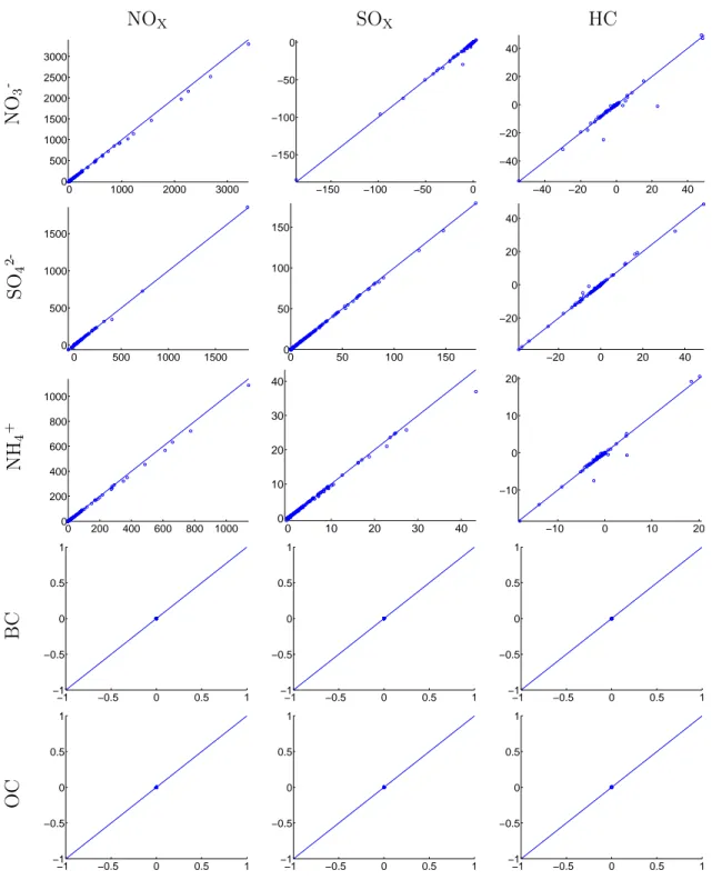
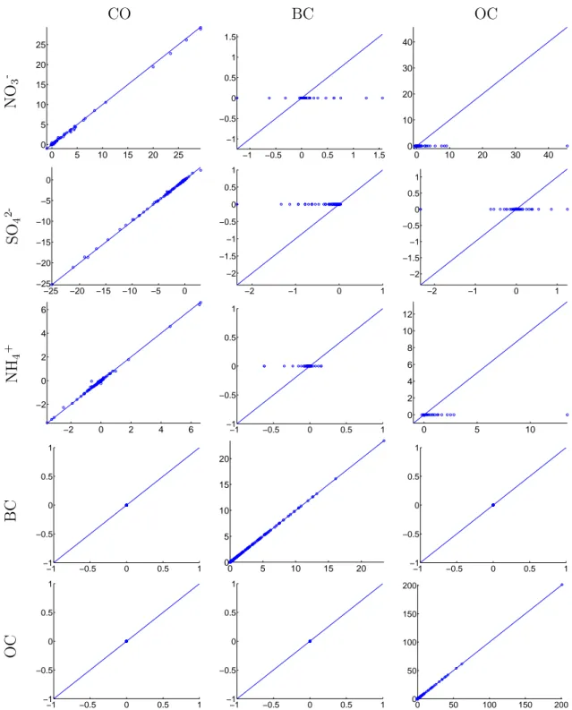
Although detailed verification can be found in Henze et al. [27] and Singh et al. [26], additional verifications of the model specific to sensitivities of PM with respect to aviation emissions are performed. To verify the adjoint sensitivities completely, the number of simulations required to run equals the number of grid boxes multiplied by the number of emissions species. As performed in pervious papers [27, 26], finite difference sensitivities and adjoint sensitivities are compared without turning on the horizontal transport module. By isolating each vertical stack of grids, the required number of simulations is reduced to the number of emissions multiplied by the number of PM species. This provides an efficient verification process of modules other than the horizontal transport, testing chemistry, convection, deposition, and emissions. And the horizontal transport was verified independently by running additional simulations without the use of other modules.
Verification of Non-horizontal Transport Modules
Fig. 2-5 and 2-6 show finite difference sensitivities versus adjoint sensitivities. There are a total of 5 aerosol components (NH4+, SO42-, NO3-, BC, OC) and 6 emission
sources (NOX, SOX, CO, HC, BC, OC), totaling 30 sensitivity comparison plots.
The comparisons of sensitivities shown here were done with one-week simulations, not with 17 months. However, noting that changing in length of the run from one day, one week, one month to three months did not change how accurate the adjoint simulation is measuring the sensitivities, sensitivity comparisons for the 17-months simulation are expected to be similar.
NOX SOX HC N O3 -0 1000 2000 3000 0 500 1000 1500 2000 2500 3000 −150 −100 −50 0 −150 −100 −50 0 −40 −20 0 20 40 −40 −20 0 20 40 S O4 2 -0 500 1000 1500 0 500 1000 1500 0 50 100 150 0 50 100 150 −20 0 20 40 −20 0 20 40 N H4 + 0 200 400 600 800 1000 0 200 400 600 800 1000 0 10 20 30 40 0 10 20 30 40 −10 0 10 20 −10 0 10 20 B C −1 −0.5 0 0.5 1 −1 −0.5 0 0.5 1 −1 −0.5 0 0.5 1 −1 −0.5 0 0.5 1 −1 −0.5 0 0.5 1 −1 −0.5 0 0.5 1 O C −1 −0.5 0 0.5 1 −1 −0.5 0 0.5 1 −1 −0.5 0 0.5 1 −1 −0.5 0 0.5 1 −1 −0.5 0 0.5 1 −1 −0.5 0 0.5 1
Figure 2-5: Adjoint vs finite difference results for kg·hr of aerosol produced due to aircraft NOX, SOX, and HC emissions
values are listed in the following Table 2.4 and 2.5. It is shown that adjoint sensitivity values are very close to finite difference values, with exceptions of aerosols created by primary PM species (BC and OC). In this case, the forward model shows that
addi-CO BC OC N O3 -0 5 10 15 20 25 0 5 10 15 20 25 −1 −0.5 0 0.5 1 1.5 −1 −0.5 0 0.5 1 1.5 0 10 20 30 40 0 10 20 30 40 S O4 2 -−25 −20 −15 −10 −5 0 −25 −20 −15 −10 −5 0 −2 −1 0 1 −2 −1.5 −1 −0.5 0 0.5 1 −2 −1 0 1 −2 −1.5 −1 −0.5 0 0.5 1 N H4 + −2 0 2 4 6 −2 0 2 4 6 −1 −0.5 0 0.5 1 −1 −0.5 0 0.5 1 0 5 10 0 2 4 6 8 10 12 B C −1 −0.5 0 0.5 1 −1 −0.5 0 0.5 1 0 5 10 15 20 0 5 10 15 20 −1 −0.5 0 0.5 1 −1 −0.5 0 0.5 1 O C −1 −0.5 0 0.5 1 −1 −0.5 0 0.5 1 −1 −0.5 0 0.5 1 −1 −0.5 0 0.5 1 0 50 100 150 200 0 50 100 150 200
Figure 2-6: Adjoint vs finite difference results for kg·hr of aerosol produced due to aircraft CO, BC, and OC emissions
tion of primary PM would changes secondary particulates whereas the adjoint model calculates no change in secondary PM due to primary PM emissions. This discrep-ancy occurs because of the absence of aerosol optical module in the adjoint model.
As mentioned previously, the adjoint model was developed as particular modules are needed, so GEOS-Chem Adjoint does not include all modules found in the forward model. Nevertheless, the changes in secondary PM caused by primary PM are about two orders of magnitude smaller than ones caused by NOX and SOX emissions.
Table 2.4: Slope of linear regression line for forward difference sensitivities versus adjoint sensitivities NOX SOX HC CO BC OC NO3- 0.951 0.993 0.959 0.982 - -SO42- 1.002 0.990 0.987 0.990 - -NH4+ 0.949 0.948 1.001 0.981 - -BC - - - - 1.000 -OC - - - 1.001
Table 2.5: r2of linear regression line for forward difference sensitivities versus adjoint
sensitivities NOX SOX HC CO BC OC NO3- 1.00 0.99 0.92 1.00 - -SO42- 1.00 1.00 0.99 1.00 - -NH4+ 1.00 1.00 0.97 1.00 - -BC - - - - 1.00 -OC - - - 1.00
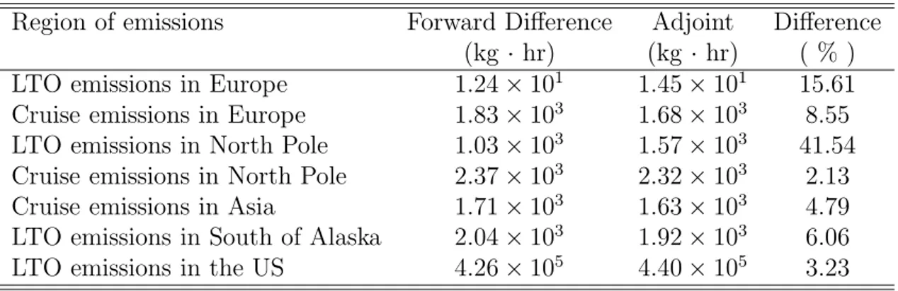
Verification of the Horizontal Transport Module
The transport module was tested using one-month simulations. The testing on an one-month simulation is expected to be similar to a testing on a longer period because most of the aerosols will be deposited in one month, thus does not accumulate impacts for longer period. Black carbon was considered for this testing since black carbon does not chemically react with other species in GEOS-Chem’s chemistry module. Two forward runs were performed: one reference run and another run with extra 100 kg/hr of black carbon emissions in the regions noted in the first column of Table 2.6. Then the change in black carbon in the US surface level is compared to adjoint results. In order to reduce the effect of discrete addition, addition of black carbon emissions was based on a three dimensional Gaussian distribution.
Having a Gaussian perturbation gave a better result than adding a constant amount of black carbon to several grid boxes. This suggests that when the grid is refined and when the perturbation is in a continuous fashion, the results from finite difference and adjoint simulations will match with better accuracy.
This is one of the reasons why the north pole’s finite difference and adjoint sensi-tivities have such a large discrepancy in Table 2.6. This difference can be reduced by using a finer resolution. The next finer grid resolution in GEOS-Chem is 2◦×2.5◦,
and running on this resolution requires 4 times the computational resources. Noting that winds are predominantly westerly in the latitudes of interest and we consider intercontinental impacts of emissions, a 4◦×5◦ grid gives an adequate approximation.
Table 2.6: Comparison of forward difference and adjoint sensitivities for the transport module
Region of emissions Forward Difference Adjoint Difference
(kg · hr) (kg · hr) ( % )
LTO emissions in Europe 1.24 × 101 1.45 × 101 15.61
Cruise emissions in Europe 1.83 × 10³ 1.68 × 10³ 8.55
LTO emissions in North Pole 1.03 × 10³ 1.57 × 10³ 41.54
Cruise emissions in North Pole 2.37 × 10³ 2.32 × 10³ 2.13
Cruise emissions in Asia 1.71 × 10³ 1.63 × 10³ 4.79
LTO emissions in South of Alaska 2.04 × 10³ 1.92 × 10³ 6.06
Chapter 3
Sensitivity Results
In this chapter, sensitivities of surface PM concentration and population exposure to PM to aircraft emissions are discussed. All simulations are run from April 1, 2006 to March 31, 2007 on a 4◦ of latitude by 5◦ of longitude horizontal grid resolution with
GEOS5 vertical resolution. The first section discusses the definition of sensitivities, the second section shows the spin-up period that is required to capture the full impact of aircraft emissions, the third section discusses the methods for premature mortality calculations, and the rest of the chapter discusses the simulation results.
3.1
Definition of Sensitivities
Before discussing the sensitivity results, this section describes what sensitivities rep-resent and how to compute the air quality or health impacts. There are two parts in each sensitivity metric: the cost function that is sensitivity of (or the numerator in the sensitivity) and the source that is sensitivity to (or the denominator in the sen-sitivity). For example, in the sensitivity of PM concentration to aviation emissions, the cost function is PM concentration and the source is aviation emissions.
The cost function in this thesis is averaged over time and space as shown in the following equation:
J = 1
VrTr
Z Z
where pm is the concentration of PM at spatial location, s, and time, t. V is the total volume of the domain of the objective function, and T is the length of the simulation. The subscript r in Eq. 3.1 and 3.2 represents the time and region of the receptor, or the objective function, and the subscript s in Eq. 3.3 represents the region and time of the source. In this case, the objective function is the PM concentration averaged over a one-year period.
The change in the cost function can be written as:
δJ = 1 VrTr Z Z δpm(s, t)dvdt (3.2) = 1 VsTs Z Z K X k=1 ∂J ∂ck(s, t) δck(s, t)dvdt (3.3) where ∂J
∂ck(s,t) is the sensitivity of the objective function to the emission of chemical species k, calculated by the adjoint simulation, and ck(s, t) represents the emission
density of specie k at location s and time t. The integrals in Eq. 3.2 are integrations over space and time where the cost function is considered, and the integrals in Eq. 3.3 are integrations over volume and time where emissions are considered.
Changing the above continuous notations to discrete notations, the sensitivities are given as three-dimensional spatial matrices or as four-dimensional spatial and temporal matrices. As indicated in Eq. 3.4, the inner product of a sensitivity matrix, shown in Fig. 3-1a, and an emission matrix, shown in Fig. 3-1b, calculates the change in the cost function caused by the emissions.
< ∂J
∂C, δC >= δJ (3.4)
where ∂J
∂C is sensitivities of the objective function to 1kg of chemical species and δC
is the emissions in kg in this discrete equation.
3.1.1
Interpreting Sensitivity Plots in this Thesis
Sensitivities, dJ
dc(s,t), represent the amount of PM created averaged over the receptor
−5 0 5
x 10−8
(a) Sensitivities (in µg m−3/kg hr−1)
−100 −50 0 50 100
(b) Emissions (in kg/hr)
Figure 3-1: Sensitivities of global surface PM concentration to NOX emissions (in
µg m−3/kg hr−1) and global aircraft NO
X emission rate (in kg hr−1) averaged over all
altitudes: Inner product of two matrices gives the change in PM concentration (in µg/m3) due to aircraft NO
X emissions
spatial sensitivity plots in this thesis are averaged over time of emissions, representing the annual average of PM concentration at the surface of a receptor location due to 1 kg/hr of emissions at the emitted location. For example, in Fig. 3-1a emitting 1 kg/hr of NOXfor one year spread over the vertical space of Santiago, Chile, increases
the annual average of global PM concentration by 9 × 10⁻⁸µg/m3. To show the
three dimensional sensitivities, many of plots, including ones in Appendix B, average sensitivities in altitudes, latitudes, or longitudes. As an example, sensitivities in Fig. 3-1a are averaged over all altitudes.
3.2
Spin-Up Period
The spin-up period is a time frame introduced to capture the complete impact of emissions on air quality. There is a time lag between when an aircraft emits primary PM and PM precursors, formation of PM in the ground layer of the receptor region, and removal of PM from the atmosphere. This time lag is shown in Fig. 3-2. Without the spin-up period, the impact of emissions emitted towards the end of a simulation will not be fully counted into the sensitivity. For example, if particulates last one week in a certain situation, sensitivity of primary PM emitted one day before the ending time will represent roughly one-seventh of its sensitivity. In this case, the
objective function, or sum of particulate matter, is summed only for one day rather than seven days.
Figure 3-2: Explanation of spin-up period
To avoid this underestimation, we need to run a spin-up period at the end for the adjoint simulation, or in the beginning of the simulation for the forward model. To determine how long it takes from emission to formation and removal of PM, seven simulations were run. These simulations all start from the same time, January 1, 2006, and end at different times, having the simulation time from one month to seven months at one-month intervals. The simulations were run with full flight global aviation emissions.
Fig. 3-3 shows the sensitivities of surface PM concentration in the US with respect to global aircraft emissions for the different lengths of the run. For a one-month run, sensitivities to emissions are smaller than longer runs even in the same interval because PM lasts longer than simulation time of one month. To compare the values of the different lengths, sensitivities of surface PM concentration in the US in the first month were compared.
If we consider the time after one month as a spin-up period, a one-month simula-tion has no spin-up period, a two-month simulasimula-tion has a one-month spin-up period, and likewise, a seven-month simulation has a six-month spin-up period. Considering that the sensitivities of six month spin-up period as reference sensitivities (six months period is a long enough time for the formation and removal of PM), sensitivities of
0 50 100 150 200 250 0 0.5 1 1.5 2 2.5x 10 −5 Days Sensitivity ( µ g/m 3) 7 month 6 month 5 month 4 month 3 month 2 month 1 month
(a) Sensitivities to 1kg of emission
0 100 200 300 400 500 600 700 0 0.2 0.4 0.6 0.8 1 1.2 1.4 1.6 Hours Sensitivity Ratio 5 Month of Spin−Up 4 Month of Spin−Up 3 Month of Spin−Up 2 Month of Spin−Up 1 Month of Spin−Up 0 Month of Spin−Up
(b) Ratio of sensitivities using various spin-up riods to sensitivities with a six-month spin-up pe-riod
Figure 3-3: Comparison of different spin-up periods of the sensitivities of surface PM concentration in the US to global aircraft emissions
each simulation are divided by the reference sensitivities. These ratios are shown in Fig. 3-3.
It is shown that sensitivities without a spin-up period are about one-half of the reference sensitivities. Also, a five-month spin-up period creates sensitivities within 0.1 percent deviation from the reference sensitivities. This means that 99.9% of particulates are scavenged within six months after when the precursors or primary particulates are emitted in GEOS-Chem simulations. Also we can see that about 95% of PM will be removed from atmosphere within four months of its emission. The average of the ratios for each month is plotted in Fig. 3-4. The ratios calculated in Fig. 3-4 are the impacts on the last month before the spin-up period. However, since these undervalued sensitivities only occur at the end of simulation, the under-estimation for the annual impact is much smaller. For example, with a twelve-month simulation without spin-up period, the last, the second to the last, the third to the last months calculates, 48%, 74%, and 89% of total impact, respectively. On average, having no spin-up period computes 92% of the annual impact. For the calculation of sensitivities in time, having 48% of the impact calculated in the last month and the full impact in the first several months brings challenge. Therefore, all simulations in this thesis use seventeen months: twelve-month simulation period and five-month
![Figure 3-9: Streamline of wind and the transport of PM from aircraft emissions [1]](https://thumb-eu.123doks.com/thumbv2/123doknet/13871612.446265/57.918.228.695.104.470/figure-streamline-wind-transport-pm-aircraft-emissions.webp)