HAL Id: hal-02862421
https://hal.umontpellier.fr/hal-02862421
Submitted on 9 Jun 2020
HAL is a multi-disciplinary open access
archive for the deposit and dissemination of
sci-entific research documents, whether they are
pub-lished or not. The documents may come from
teaching and research institutions in France or
abroad, or from public or private research centers.
L’archive ouverte pluridisciplinaire HAL, est
destinée au dépôt et à la diffusion de documents
scientifiques de niveau recherche, publiés ou non,
émanant des établissements d’enseignement et de
recherche français ou étrangers, des laboratoires
publics ou privés.
cucumber (Cucumis sativus L.) cultivars and their F1
hybrid?
Xiu-Juan Wang, Meng-Zhen Kang, Xing-Rong Fan, Li-Li Yang, Bao-Gui
Zhang, San-Wen Huang, Philippe de Reffye, Fei-Yue Wang
To cite this version:
Xiu-Juan Wang, Meng-Zhen Kang, Xing-Rong Fan, Li-Li Yang, Bao-Gui Zhang, et al.. What are
the differences in yield formation among two cucumber (Cucumis sativus L.) cultivars and their F1
hybrid?. Journal of Integrative Agriculture , Elsevier, 2020, 19 (7), pp.1789-1801.
�10.1016/S2095-3119(20)63218-X�. �hal-02862421�
RESEARCH ARTICLE
Available online at www.sciencedirect.com
ScienceDirect
What are the differences in yield formation among two cucumber
(Cucumis sativus L.) cultivars and their F
1hybrid?
WANG Xiu-juan
1, 2, KANG Meng-zhen
1, 3, FAN Xing-rong
4, YANG Li-li
5, ZHANG Bao-gui
6, HUANG
San-wen
7, Philippe DE REFFYE
8, WANG Fei-yue
1, 91 The State Key Laboratory of Management and Control for Complex Systems, Institute of Automation, Chinese Academy of
Sciences, Beijing 100190, P.R.China
2 Beijing Engineering Research Center of Intelligent Systems and Technology, Institute of Automation, Chinese Academy of
Sciences, Beijing 100190, P.R.China
3 Innovation Center for Parallel Agriculture, Qingdao Academy of Intelligent Industries, Qingdao 266109, P.R.China
4 School of Computer Science and Information Engineering, Chongqing Technology and Business University, Chongqing 400067,
P.R.China
5 College of Information and Electrical Engineering, China Agricultural University, Beijing 100083, P.R.China 6 College of Land Science and Technology, China Agricultural University, Beijing 100193, P.R.China
7 Agricultural Genomes Institute at Shenzhen, Chinese Academy of Agricultural Sciences, Shenzhen 518124, P.R.China 8 AMAP, University Montpellier, CIRAD, CNRS, INRA, IRD, Montpellier 34000, France
9 The School of Computer and Control Engineering, University of Chinese Academy of Sciences, Beijing 100049, P.R.China
Abstract
To elucidate the mechanisms underlying the differences in yield formation among two parents (P1 and P2) and their F1 hybrid of cucumber, biomass production and whole source–sink dynamics were analyzed using a functional–structural plant model (FSPM) that simulates both the number and size of individual organs. Observations of plant development and organ biomass were recorded throughout the growth periods of the plants. The GreenLab Model was used to analyze the differences in fruit setting, organ expansion, biomass production and biomass allocation. The source–sink parameters were estimated from the experimental measurements. Moreover, a particle swarm optimization algorithm (PSO) was applied to analyze whether the fruit setting is related to the source–sink ratio. The results showed that the internal source–sink ratio increased in the vegetative stage and reached a peak until the first fruit setting. The high yield of hybrid F1 is the compound result of
both fruit setting and the internal source–sink ratio. The optimization results also revealed that the incremental changes in fruit weight result from the increases in sink strength and proportion of plant biomass allocation for fruits. The model-aided analysis revealed that heterosis is a result of a delicate compromise between fruit setting and fruit sink strength. The
organ-Received 30 January, 2019 Accepted 8 March, 2020
Correspondence KANG Meng-zhen, Tel: +86-10-82544776, Fax: +86-10-82544799, E-mail: mengzhen.kang@ia.ac.cn
© 2020 CAAS. Published by Elsevier Ltd. This is an open access article under the CC BY-NC-ND license (http:// creativecommons.org/licenses/by-nc-nd/4.0/).
1. Introduction
Cucumber (Cucumis sativus L.) is a very popular vegetable plant worldwide, and its yield components comprise the number, weight and quality of individual fruits (Marcelis 1992). Hybrid vegetable technology is one of the best options to improve cucumber yield. Hybrid vigor can be expressed by the total yield and increased yield due to the large number of fruits/plants (Ghaderi and Lower 1978). Yield and fruit quality are some of the most frequent traits influenced by heterosis. Heterosis or hybrid vigor is commonly known as the superior performance of hybrid organisms compared with either of their parents (Birchler 2015). In cucumber, Hayes and Jones (1916) first observed heterosis in fruit size and fruit number per plant. Ghaderi and Lower (1978) suggested that heterosis in yield components such as the number or weight of leaves, branches, and roots should have a direct effect on fruit yield. F1 hybrids may
have greater photosynthetic activity than their parents, thus leading to a higher yield.
Crop yield is the result of the interactions of genetic and environmental factors. Breeders have proposed the concept of an ideal plant (ideotype) adapted to a target environment. For cucumber, a heliophile crop, dry matter production through photosynthesis is one of the most important processes to consider when characterizing an ideotype. Internode length, leaf size and leaf angle are three important traits of the ideal cucumber plant architecture (Falster and Westoby 2003; Sarlikioti et al. 2011). Breeding for yield mainly utilizes hybrid vigor to change some plant morphological traits by hybrid breeding, thus improving the yield, cultivar and resistance (Xie et al. 2009). A major difficulty lies in decomposing the complex interactions between genotype and environment because the main phenotypic traits (e.g., yield, plant height, organ number and size) integrate multiple internal morphological and physiological processes and external interactions with field and climatic conditions (Letort et al. 2008).
Heuvelink et al. (2007) reported that using plant models allows the evaluation of newly available genotypes by analyzing their performance and identifying the most influential parameters to improve yield under various environmental conditions. Many plant growth models have been developed to increase our knowledge of plants, improving agricultural practices and environmental
optimization and control (Wu et al. 2012; Fan et al. 2015). Studies of the potential of linking growth models to quantitative genetics aim to integrate genetic knowledge in plant growth models considering the effect of the environment (Hammer et al. 2005; Letort et al. 2008; Xu et al. 2011; Yin
et al. 2016; Chew et al. 2017). If the model parameters
themselves can be viewed as different quantitative traits, they should have high heritability because they are expected to be less dependent on the environmental conditions and to show more direct gene expression (Letort et al. 2008). Thus, it is easier to analyze the genetic effects using model parameters than using traditional traits. Moreover, optimization processes allow the determination of key parameters influencing yield, even when complex genetic correlations are introduced. However, plant growth model selection will be a crucial step.
Functional–structural plant models (FSPMs) explicitly describe the development of a plant structure over time as governed by physiological processes that, in turn, depend on environmental factors (Vos et al. 2007). Such models dynamically simulate plant systems, allowing for feedback between processes at the level of individual organs and functioning of the plant as a whole (Vos et al. 2010). The features of FSPMs are interesting for studying fruit setting in horticultural plants (Wubs et al. 2009). Based on botanical knowledge and source–sink regulation rules, the FSPM GreenLab is a generic model that can simulate interactions among the fruit set (e.g., position, number and size), biomass production and allocation to better understand the dynamics of biomass production and morphogenesis among cucumber cultivars. Furthermore, one interesting feature of the GreenLab Model is that the Model parameters can be adjusted globally by fitting model outputs to corresponding measured organ biomass (Christophe et al. 2008) thanks to its mathematical formalism; this is a demanding and critical step in developing and applying a model (Seidel et al. 2018). The GreenLab Model has been applied to various plants, including maize (Ma et al. 2008), tomato (Kang et al. 2011), sweet pepper (Ma et al. 2011), and chrysanthemum (Kang
et al. 2012). However, none of these plants has been used
to analyze heterosis between parents and F1 hybrids. The aim of the study was to analyze the processes underlying the different biomass production levels between two parents (P1 and P2) and their F1 hybrid of cucumber
using a modeling approach. First, the GreenLab Model was calibrated with the data of the two parents and their level model may provide a computational approach to define the target of breeding by combination with a genetic model. Keywords: cucumber, biomass production, functional–structural plant model, source–sink ratio, fruit-setting, PSO, heterosis
F1 hybrid to more deeply understand the differences
among their development and growth processes with the estimated model parameters; second, a particle swarm optimization algorithm (PSO) was applied to investigate the relationship between the fruit setting and source–sink ratio by simultaneously optimizing the source–sink parameters and fruit positions and numbers. This model-based analysis thus provides a new tool to better understand the heterosis phenomenon.
2. Materials and methods
2.1. Experiment setup and measurements
Plant materials Cucumber (Cucumis sativus L.) seeds were provided by the Institute of Vegetables and Flowers, Chinese Academy of Agricultural Sciences. The large-leaf line (C. sativus var. sativus) DF-32 (P1), the small-leaf line (C. sativus var. hardwickii) XF-24 (P2) and their hybrid (F1) were cultivated in a greenhouse of China Agricultural
University (40.01°N, 116.28°E) from March to July 2010. The parent P1 is a late-maturing cultivar; the first female
flower is located at the 15th–16th phytomer (counting from the base). This cultivar produces large blades and large fruit with a low fruit-set rate. The parent P2 is an early-maturing
cultivar; the first female flower is located at the 3rd–5th phytomer. This cultivar produces small blades and small fruit with a high fruit-set rate. The traits of the F1 hybrid are
intermediary (Fig. 1).
The two parents and F1 hybrid were sown on March 9, 2010. Cucumber seedlings with four leaves were implanted into 25-cm pots on April 10, 2010. The pots were filled with 70% peat, 20% vermiculite and 10% pearlite. Next, 20,
20 and 10 pots of plants were planted for P1, P2 and F1,
respectively. There was no water or nutrient stress. All tendrils and side shoots were pruned to allow monopodial growth. Measurements were performed on two plants in the middle rows with at least one border plant on each side. The fruits were harvested every three or four days. Measurements The environmental conditions, namely, temperature, humidity and light intensity, were monitored during plant growth in the greenhouse to analyze their effects. Both destructive measurements and continuous nondestructive observations were carried out. Continuous observations were performed on six plants for two parents and F1 hybrid, twice per week, with detailed topological
observations on the number of leaves, phytomer ranks of flowers on the main stem, and stage of development (flower bud, flower and fruit or abortion) at each flower position, in order to describe dynamic fruit setting for two parents and F1 hybrid.
In destructive measurements, two cucumber plants for two parents and F1 hybird were selected to measure the
dry weight of individual organs (internode, blade, petiole and root) and blade surface for each sampling. In total, six samplings were made during the growing period (S1, 10 April; S2, 26 April; S3, 17 May; S4, 31 May; S5, 16 June; and S6, 3 July). The measured data were used to estimate the source–sink parameters of the model for two parents and F1 hybrid.
2.2. GreenLab Model
GreenLab is a generic plant model that simulates two basic plant processes: development (organogenesis) and growth (organ expansion) (Yan et al. 2004). At each time
P1 P1 P2 P2 F1 F1 126 cm 126 cm 90 cm 87 cm 138 cm 140 cm
interval, called the growth cycle (GC, the period between the sequential emergence of leaves on the main stem of a plant), the plant structure is updated according to the organogenesis model. Organogenesis is simulated with a dual-scale automaton (Yan et al. 2002), which gives the number of organs at each cycle that participate in biomass production and allocation.
Modeling biomass production In the GreenLab Model, at the ith GC, the biomass production of a plant Q(i) is calculated using eq. (1) (Guo et al. 2006):
Q(i)=PET(i)∙µ∙SP
(
1–exp ( –kS(i)SP)
)
(1)where i is the age of the plant in GC. PET(i) (mm per GC) is the potential evapotranspiration during the ith GC that is affected by several microclimate conditions (light, temperature and vapor pressure deficit) (Allen et al. 1998). The PET of a GC is summed from daily PET values, the duration depending on the daily temperature and phyllochron per cycle; SP (cm2) is the ground maximal projection area of
the plant, linked to the density of planting (Ma et al. 2008); µ (g cm–2 mm–1) estimates the water use efficiency, expressing
produced biomass by plant evapotranspiration per unit of water (Kang et al. 2011); k is the light extinction coefficient, set to an empirical value of 1; S(i) is the total functioning leaf area at the ith GC, summed from the individual leaf area in the model. Each leaf area is computed from its biomass and a specific leaf weight, the latter being assessed directly from the data. Because the biomass of each leaf is dependent on the global plant demand during its expansion, it can be affected by concurrent events such as the fruit set. The initial biomass Q(0) is from the seed.
Modeling biomass partitioning The model is based on the hypothesis that dry matter partitioning is regulated by the sink strengths of the plant organs. The sink strength of an organ is defined here as the potential growth capacity, i.e., the biomass at nonlimiting assimilate supply (Marcelis 1994). Biomass is distributed among growing organs according to their own sink strength. The sink strength of organ o of age
j is calculated by eq. (2):
po(j)=Pofo(j) (2)
where Po is the organ sink strength, and o represents the
organ type (b, blade; p, petiole; in, internode; f, female). In this study, we set the maximum measured value of fruit, that is, Pf equals 14.6, 7.6 and 12.3 g for the parents P1 and P2
and hybrid F1, respectively, as the reference potential sink
strength. The sink strengths of other organs (Pb, Pp and
Pin) are hidden parameters to be estimated from the plant
data. Thus, the sink strength has units (g per GC) and represents the organ’s ability to compete for assimilates in each GC. Because each organ has different needs for biomass during its lifetime, function fo(j) is defined as the
organ sink variation, described empirically by a discrete
Beta function as in eq. (3): fo(j)= goj/μ o 1≤j≤to 0 j>to (3) where goj=(j–0.5 to ) ao–1 (1–j–0.5t o ) bo–1 μo=
∑
togoj o=b, p, in, f j=1This function gives the shape of the organ sink variation curve at a constant biomass supply. The product Pofo(j)
gives the demand of organ o with age j in the plant. Given the expansion duration to and one of the control parameters
ao=2, another control parameter bo was estimated from
the plant data for each type of organ. This constraint is empirical and generally yield good results for different organs and plants (Guo et al. 2006; Kang et al. 2011). The larger the value of bo is, the faster the expansion is. Appendix A
shows different curve shapes of fo(j) depending on the values
of parameters ao and bo, which could differ among organ
types and plant species. The duration of growth to of organ
o can be observed directly from measurements, which is approximated to be 20 cycles.
Summing the sink strength of all organs, we obtain the total demand of plant D(i) at the ith GC:
D(i)=
∑
Po(
∑
No(i, j) fo(j) ij=1
)
o (4)
where No(i, j) is the number of organs o of age j at plant age i. In the cucumber plant here, for leaves and internodes,
this value is 1; for the fruit, it can be 0 or 1, depending on whether a fruit is set at the phytomer rank.
According to the sink strength, the biomass acquired by the organ of age j at the ith GC is:
Δqo(i, j)=PoD(i)fo( j)Q(i) (5) In eq. (5), the dynamic source–sink ratio Q(i)/D(i), simply written as Q/D. It reflects the competition level in the plant, showing the biomass availability for each organ. According to eq. (5), larger Q/D values during the expansion of an organ produce a larger final biomass. This ratio can be computed by the model recurrently when all parameter values are known. The source–sink ratio at the fruit set is quantified by computing this ratio when each fruit appears, and a threshold is given as slow. For cucumber, a fruit will possibly appear at each node, but only some positions can set a fruit; therefore, when the position sets a fruit, the plant demand (D) increases, then the ratio Q/D decreases and is lower than the threshold. Therefore, some later produced fruit may abort while the competition for assimilates
increases. Thus, spatial fruit position can be determined by the source–sink ratio (Ma et al. 2011).
Summing the biomass of all individual organs of the same property produces the total biomass of organs that can be obtained by experimental measurements. The biomass of an organ o is the accumulated biomass of the organ of age
j at the ith GC:
qo(i, j)=
∑
j Δqo(i–j+k, k) (i≥j)k=1 (6)
Accordingly, the total weight of the fruit at the final harvest, denoted by Wf (g/plant), is computed by eq. (7):
Wf=
∑
Nf(N, j) qf(N, j)tf
j=1 (7)
where tf (unit: GC) is the fruit functioning duration, and N is
the final GC (or maximal GC) of the plant. 2.3. Parameter estimation of GreenLab
In GreenLab, the parameters are classified into two categories: measurable parameters (e.g., functioning duration of blades, number of organs emerged at each GC) and hidden parameters that cannot be measured directly in the field (e.g., organ sink strength). The hidden parameters are estimated by minimizing the difference between the measured data and corresponding simulation results. A generalized nonlinear least-square method (GLSQR) adapted from the Levenberg-Marquardt algorithm is used for estimation (Zhan et al. 2003). Model computation and model fitting on experimental data were conducted using the open-source GreenScilab Software.
A common set of parameters (Table 1) is estimated simultaneously by fitting the plant data at different development stages, which is called multifitting. For directly measurable parameters, following the observations, the organ expansion duration (from appearance to stop growing) was set to 20 GCs, while the organ function duration (from appearance to death) was set to 40 GCs for the blade, petiole, internode and fruit according to the data of continuous observations. Leaf thickness was estimated as the ratio of the leaf fresh mass to surface area (Wright and Westoby 2002). It plays an important role in leaf and plant functioning and is related to species’ strategies of resource acquisition and use (Vile et al. 2005).
2.4. Data analysis
Statistical analyses were performed using R2.11.1 (Copyright (C) 2010, the R Foundation for Statistical Computing). Analysis of variance (ANOVA) was used to assess the differences in phyllochron between the parents and F1 hybrid.
2.5. Maximization of the fruit weight
To clarify the origin of heterosis, a PSO algorithm was applied to analyze whether the fruit setting could be related to the dynamic of the source–sink ratio. First, based on the estimated source–sink parameters, the fruit positions are optimized by setting different numbers of fruit per plant for the parents P1 and P2 and hybrid F1 to analyze the
effect of the sink organ on potential biomass production; second, both the source–sink parameters and positions of the fruit per plant were synchronously optimized using different numbers of fruits per plant to check the potential augmentation of yield.
The optimization objective was to maximize the total weight of the fruit for each plant. Assuming one fruit for one position, the mathematical formalism of the optimization problem is given by the following eq. (8):
Maximize Wf
Subject to 1≤
∑
NposFruit(i)i=1 ≤NF
(8) where posFruit(i) is a binary (0/1) variable depending on whether a fruit is set at the phytomer rank, which corresponds to the function of No(i, j) in eq. (4) for the fruit;
N
∑
i=1posFruit(i) gives the total number of fruits per plant; NF
is the maximum number of fruits; and Wf is a function of posFruit(i) and qf (eq. (7)). A PSO algorithm is used to solve
the optimization problem (Qi et al. 2010).
3. Results
3.1. Experimental results
Phyllochron The phyllochron shows no significant difference between the parents (P1 and P2) and the F1
hybrid (ANOVA, df=2, F=0.085, P>0.5), as shown in Fig. 2. Table 1 Source–sink parameters identified from the measurement data using the GLSQR method
Parameter1) Definition Unit
Pb, Pp, Pin Organ sink strength (eq. (2)) g
bb, bp, bin, bf Organ sink variation parameter (eq. (3)) –
SP Characteristic surface of an individual plant (eq. (1)) cm2
µ Water use efficiency (eq. (1)) g cm–2 mm–1
slow A threshold, fruits appear at GC t if source–sink ratio Qt/Dt>slow –
This means that the development speed is similar, and we can use the same time step in the model to compute the source–sink parameters.
Because the environmental factors were considered by combining the daily PET values in eq. (1) of the model, the potential evapotranspiration (PET) per cycle was calculated by accumulating daily PET inside a GC according to the daily temperature, light intensity and air humidity (Fig. 3). Vegetative organ biomass The biomass and sizes of organs from a given type (leaves, petioles and internodes) vary along the stem within one plant and are different at the same phytomer rank for two parents and F1 hybrid. The
plants of parent P1 had the largest organ biomass for the
internode, blade and petiole. In contrast, parent P2 had the
smallest organ sizes, while hybrid F1 showed intermediate
values, as shown in Fig. 4. Furthermore, the averaged plant heights and internode diameters showed similar patterns (P1>F1>P2) (Table 2).
Fruit setting and fruit biomass According to the observation, the first fruit appeared at the phytomer ranks 15–16, 3–5 and 10–12 for parents P1 and P2 and hybrid
F1, respectively, i.e., the first fruit set was the earliest in P2,
latest in P1 and that of F1 was between them (P1>F1>P2). The
harvested mean final number of fruit per plant for parents P1
and P2 and hybrid F1 showed an inverse trend (P1<F1<P2).
The mean dry weights of individual fruit were P1>F1>P2 (Table 3), indicating that F1 produced an intermediate amount of fruit compared with its parents, with a fruit size close to P1. Therefore, it is not surprising that the mean total fruit dry weight per plant of F1 was the highest at the
final harvest (P1<P2<F1), as shown in Table 3. The results
indicated that F1 has better performance than the parents,
a phenomenon called heterosis. 3.2. Model-assisted analysis
Differences in the source–sink parameters for parents P1 and P2 and hybrid F1 The trend of leaf thicknesses for
parents P1 and P2 and hybrid F1 was P2>P1>F1 (data not
shown), which was used for parameter estimation. The target data for two plants from four different sampling dates were fitted simultaneously, including the dry weights of individual organs (internode, blade, petiole and fruit) and total dry weight of each component. In total, 1 572, 1 276, and 1 236 target data points were fitted simultaneously for P1, P2 and F1, respectively. The organ-level fitting results of
the last two stages (S5 and S6) for P1, P2 and F1 are shown
in Fig. 4. Only dry weights of individual internodes, leaves, petioles and fruits of one plant were given for each sampling for clarification. The total dry weights of each organ type for stages S3–S6 are given in Fig. 5. The data of S1 and S2 were omitted because they were too tiny to display. The correlation coefficient (R2) values between the observed and
fitted values for the two parents and their hybrid F1 were
0.97, 0.91 and 0.92, respectively (Table 4).
Thermal time (°C d) 0 500 1 000 1 500 2 000 Number of leaves 0 10 20 30 40 50 60 70 P1: y=0.0323x–0.9591 R2=0.9933 P2: y=0.0282x+3.9627 R2=0.9962 F1: y=0.033x+0.321 R2=0.9975 P1 P2 F1
Fig. 2 Relationship between the leaf number and thermal
time for the parents P1 and P2 and F1 hybrid during plant development.
Days after implanting (d)
0 20 40 60 80 Temperature (°C) 0 10 20 30 40
Days after implanting (d)
0 20 40 60 80 Light (W m –2) 0 50 100 150 200 250 300 350
Days after implanting (d)
0 20 40 60 80 PET (mm –2 d –1) 0 2 4 6 8 10 12
Table 2 Comparison of the organ biomass and plant size for parents P1 and P2 and hybrid F1 at the last stage (S6, two plants)
Total dry weight (g) Average
plant height (cm) Internode diameter (mm)
Internode Blade Petiole
P1 18.4±1.1 42.5±3.0 9.6±0.8 431.5±16 6.28±0.2
P2 4.1±0.1 17.4±0.5 2.9±0.3 254.5±14 4.28±0.1
F1 9.6±1.8 26.5±5.8 5.4±1.4 378.6±36 5.46±0.3
The values are expressed as mean±SD. 0 10 20 30 40 50 60 Internode weight (g) 0 0.1 0.2 0.3 0.4 0.5 0.6 0 10 20 30 40 50 60 Blade weight (g) 0 0.2 0.4 0.6 0.8 1.0 1.2 1.4 1.6 0 10 20 30 40 50 60 Petiole weight (g) 0 0.1 0.2 0.3 0.4 0 10 20 30 40 50 Fruit weight (g) 0 2 4 6 8 10 12 14 16 0 10 20 30 40 50 60 0 0.1 0.2 0.3 0.4 0.5 0.6 0 10 20 30 40 50 60 0 0.2 0.4 0.6 0.8 1.0 1.2 1.4 1.6 0 10 20 30 40 50 60 0 0.1 0.2 0.3 0.4 Phytomer rank 0 10 20 30 40 50 0 2 4 6 8 10 12 14 16 0 10 20 30 40 50 60 0 0.1 0.2 0.3 0.4 0.5 0.6 0 10 20 30 40 50 60 0 0.2 0.4 0.6 0.8 1.0 1.2 1.4 1.6 0 10 20 30 40 50 60 0.0 0.1 0.2 0.3 0.4 0 10 20 30 40 50 60 0 2 4 6 8 10 12 14 16 P1 P2 F1
S5P1_Obs S5P1_Est S6P1_Obs S6P1_Est
S3P1_Obs S3P1_Est S4P1_Obs S4P1_Est
Fig. 4 Fitting results of growing stages S3 (17 May), S4 (31 May), S5 (16 June) and S6 (3 July) for two parents (P1 and P2) and
their hybrid F1. All the data were fitted simultaneously, including the total dry weight for all organs and organ-level dry weight of individual internodes, blades, petioles, and fruit (from top to bottom). Only one plant was given for each stage. Obs, observed data; Est, estimated data. The arrows indicate the fruit-set positions for stages S5 (up arrow) and S6 (down arrow).
A set of source–sink parameters was identified for P1, P2 and F1, as shown in Table 4. The sink strengths of the blade,
petiole and internode (Pb, Pp and Pin) for F1 were intermediate
between those of the parents P1 and P2 (P1>F1>P2). The sink
variation of the blade (bb) for F1 was intermediate between that of the parents. The sink variation of the petiole (bp) was
slightly smaller than that of the parents. The sink variation values of the internode (bin) and fruit (bf) for F1 were larger
than those of P1 and P2, respectively, indicating quicker
expansion compared with the leaves. Regarding the source parameters, the projection area (SP) for F1 was intermediate
between that of the parents P1 and P2 (P1>F1>P2). The
water use efficiency (µ) was larger for F1 than for P1 and P2
(P2<P1<F1). There are shifts in the profiles of the internode and blade that were not reproduced by the model, likely due to the abortion of early fruit for parent P1.
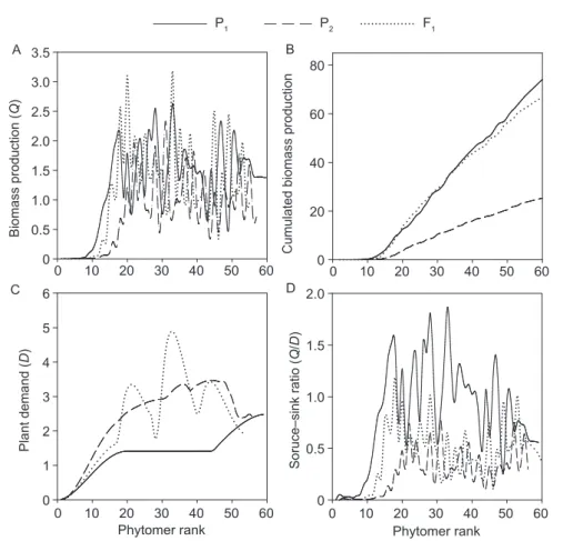
Computed plant biomass production, demand and source–sink ratio Using these parameter values, the plant biomass production and plant demand of each cycle were computed (Fig. 6). The biomass production per cycle (Q, Fig. 6-A) and cumulated biomass production (Fig. 6-B) were larger for parent P1 and hybrid F1 than for parent P2.
The plant demand (D, Fig. 6-C) was larger for parent P2 and hybrid F1 than for parent P1, which was consistent with the
fruit setting. Anytime there is fruit removal after maturation,
the plant demand drops.
The ratio between the biomass supply and demand (Q/D, Fig. 6-D) increased during the vegetative stage until fruit began to be the dominant sinks. The peak value was first reached for parent P2 followed by hybrid F1 and
then parent P1. The value of the first peak of hybrid F1
was between the two parents (P1 and P2). The Q/D of the parent P1 and F1 hybrid was visibly larger than that of P2.
Table 3 Comparison of the mean final number of fruits per plant, mean dry weights of individual fruits and mean total fruit weight
per plant for parents P1 and P2 and hybrid F1 (growing stage S6 (3 July), two plants)
Mean final number of fruits per plant Mean dry weights of individual fruits (g) Mean total fruit dry weight per plant (g)
P1 1.0±0.7 9.6±4.9 12.2±3.5
P2 6.0±0.9 3.9±1.8 22.9±9.1
F1 4.2±0.8 7.2±3.4 31.9±0.6
The values are expressed as mean±SD.
Table 4 Estimated parameter values for parents P1 and P2
and hybrid F1 Parameter1) P 1 P2 F1 Pb 0.87 (0.55) 1.66 (0.40) 1.15 (0.18) Pp 0.18 (1.15) 0.28 (0.67) 0.21 (0.81) Pin 0.36 (2.00) 0.44 (0.19) 0.41 (0.23) bb 2.11 (0.19) 2.76 (0.07) 2.36 (0.18) bp 1.81 (1.54) 2.46 (0.58) 1.66 (1.29) bin 2.67 (3.98) 2.59 (1.90) 3.46 (3.03) bf 1.35 (0.08) 2.41 (0.05) 5.35 (0.04) SP 479.0 (4.08) 134.5 (2.22) 251.9 (2.91) µ 0.00052 (0.45) 0.00042 (0.85) 0.00069 (0.99) R2 0.97 0.91 0.92 1) P
o is the coefficient of sink strength; bo is the parameter of the
beta function for organ expansion, where, o=in (internode); b (blade); p (petiole); f (fruit). SP is the projected surface area of
the plant. The sink strength of fruit (Pf) is set to their respective
maximum fruit weight.
Data in parentheses are CVs (%).
F1 Phytomer rank 0 10 20 30 40 50 60 0 10 20 30 40 50 P2 Phytomer rank 0 10 20 30 40 50 60 0 10 20 30 40 50 P1 Phytomer rank 0 10 20 30 40 50 60
Total dry weight for each organ (g) 0 10 20 30 40 50
Blade_Est Petiole_Est Internode_Est Fruit_Est
Blade_Obs Petiole_Obs Internode_Obs Fruit_Obs
Fig. 5 Fitting results of the total dry weight for all organs by multifitting using plant data from four samplings (growing stages S3
(17 May), S4 (31 May), S5 (16 June) and S6 (3 July), respectively) for the parents (P1 and P2) and their hybrid F1. Obs, observed
Large-fruited cultivar P1 needs a higher source–sink ratio
for the fruit set.
3.3. Computational experiments on the fruit weight
Optimizing fruit positions and numbers Based on the estimated source–sink parameters, the positions of fruit are optimized by setting different number of fruit per plant for the parents P1 and P2 and hybrid F1 to analyze the
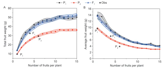
effect of the sink organ on potential fruit weights. Here, the potential fruit weight means the best yield with different fruit positions. It increased with the number of fruits per plant and reached the saturation point at approximately 10 fruit (Fig. 7-A) for the parents P1 and P2 and hybrid F1, while the
average fruit weight decreased (Fig. 7-B). The optimized values of the parent P1 and hybrid F1 were larger than that
of parent P2, indicating a higher source supply in P1 and
F1. The total potential biomass production of P1 and F1 are
close, depending on the source parameters (SP and µ). The
increase in biomass production reached a limit, indicating a limit in the source supply. Interestingly, the potential and observed plant biomass are close for the parent P2 (6 fruits)
and hybrid F1 (4 fruits), with 29.3 g vs. 29.7 g (increase by
1%) and 32.4 g vs. 35.7 g (increase by 10%), respectively. This could mean that, for a real plant, its fruit position is already optimized by itself for its biomass production. This result agrees with that in a previous study of the fruit position optimization of maize (Qi et al. 2009).
Optimizing the fruit positions, numbers and source–sink parameters Both the source–sink parameters and positions of the fruit per plant were synchronously optimized using different numbers of fruits per plant to check the potential augmentation of biomass. Here, the potential plant was obtained by synchronously optimizing the source–sink parameters and numbers and positions of the fruits per plant. Table 5 gives the variation in the optimized parameters, which is limited to the range between the estimated values (Table 4) of the parents and F1 hybrid.
As shown in Fig. 8, both the optimized total and average fruit weights were larger than the observed values. This is reasonable because the source capacity increased. The optimized total fruit weights increased with the fruit number and reached a saturation point of approximately 10 fruits. The mean fruit weights decreased but were always above the observed values. The optimized source parameter (SP) was
close to the value of parent P1, while the source parameter
0 10 20 30 40 50 60
Cumulated biomass production
0 20 40 60 80 0 10 20 30 40 50 60 Biomass production ( Q ) 0 0.5 1.0 1.5 2.0 2.5 3.0 3.5 P1 P2 F1 Phytomer rank 0 10 20 30 40 50 60 Soruce–sink ratio ( Q /D ) 0 0.5 1.0 1.5 2.0 Phytomer rank 0 10 20 30 40 50 60 Plant demand ( D ) 0 1 2 3 4 5 6 A B C D
Fig. 6 Estimated values during plant growth. A, biomass production per cycle Q. B, accumulated biomass production per plant.
Table 5 Definitions and variation ranges of the source–sink
parameters that are optimized in the optimization problem
Parameter Definition Range
Pb Sink strength of the blade [0.5, 1.7]
Pp Sink strength of the petiole [0.1, 0.3]
Pin Sink strength of the internode [0.3, 0.5]
Sp Projected surface area of the plant [100, 500]
r Water use efficiency [0.0004, 0.001]
Fig. 7 Optimized and observed (Obs) total weight (A) and average weight (B) of fruit for the fruit number range from 1 to 15 when
the fruit position is optimized. The area around each fruit weight corresponds to the respective standard error.
(µ) was similar to that of hybrid F1 (data not shown). The optimized results led to more biomass production according to eq. (1) and, thus, a larger fruit weight.
4. Discussion
The GreenLab Model was used to study the source–sink dynamics of individual organ growth and link it to the fruit setting and fruit biomass for the parents and hybrid F1. Our
modeling results confirmed that the organ growth and fruit setting is controlled by the source–sink ratio in cucumber (Fig. 6), and the model can well reproduce the results of experimental measurements. One original aspect of this study compared with earlier GreenLab models (Mathieu
et al. 2007; Kang et al. 2011) was to introduce the potential
fruit growth rate (measured maximum fruit dry weight) into the GreenLab model to represent the fruit sink strength. The sink strength of each organ then has units (g per GC) and represents the ability to compete for assimilates instead of a relative value (compared with the leave).
4.1. Correlation between the cyclic patterns of organ growth and source–sink ratio by the GreenLab Model The biomass and size of each organ differ within one plant for two parents and F1 hybrid, which could be due to the
difference in the supply and demand, that is, the source–sink ratio during plant growth. Additionally, the biomass and size of each organ are different at the same phytomer rank for two parents and F1 hybrid, likely due to the difference
in their sink strengths because the expansion time showed no significant difference according to the observations.
0 5 10 15 10 20 30 40 50 60
Total fruit weight (g)
Number of fruits per plant
P1 P2 F1 Obs P1 F1 P2 A 0 5 10 15 0 2 4 6 8 10 12 14 16
Average fruit weight (g)
Number of fruits per plant P1
F1
P2
B
Number of fruits per plant
0 2 4 6 8 10 Fruit weight (g) 0 10 20 30 40 50 60 70 80 Opt_Total Opt_Ave Obs_Total Obs_Ave P1 P2 F1 F1 P 2
Fig. 8 Optimized (Opt) and observed (Obs) total weight and
average (Ave) weight of fruits for the fruit number ranging from 1 to 10 when the fruit position and the source–sink parameters (Sp, µ, Pb, Pin, and Pp) are optimized. The stars represent the observed fruit weights for the parents P1 and P2 and F1 hybrid.
Moreover, the waves in the organ profile appeared as an emergent property because of the fruit setting (Fig. 4), a finding that is consistent with the study of Mathieu et al. (2007). There is a time lag between an increase in the source–sink ratio (and, hence, larger leaves) and the number of young fruit because it takes time for the fruit to expand.
Furthermore, the individual fruit weight and final fruit number differ between two parents and F1 hybrid, likely
due to the difference in the fruit sink strength and source– sink ratio during the fruit setting (Marcelis et al. 2004). A general pattern is that a decrease in the source–sink ratio is accompanied by a new non-aborted fruit, and vice versa. What is interesting is the threshold (slow) of setting the first
and the subsequent fruit in P1, P2 and F1. Fig. 6-D shows
that the source–sink ratio was higher for single-fruit type P1 and lower for multiple-fruit type P2, while their hybrid
was intermediate. This finding demonstrates that different cultivars may have different needs of the source–sink threshold (or hormone level) for the fruit setting, which gives different final numbers and sizes of fruit (Mathieu et al. 2008). This result is consistent with that of previous studies, and the link between the fruit set and computed source–sink ratio has been presented by previous application of GreenLab to sweet pepper for six cultivars (Ma et al. 2011) and tomato for different densities (Kang et al. 2011).
4.2. Model-assisted analysis of biomass production in cucumber
According to the estimated parameters of source strength (SP and µ) and sink strength (Pin, Pb and Pp), we can see
that the model explained well the differences in biomass production for P1, P2 and F1. The estimated sink parameters
of the internode (Pin), blade (Pb) and petiole (Pp) in F1 plants were intermediate between the parents (Table 4). The estimated results are consistent with the experimental data. Hybrid F1 has the best fruit biomass, indicating heterosis of
F1. The high biomass production of the F1 hybrid is achieved
by factors both in plant development (fruit setting) and sink competition (larger sink strength of fruit).
The hybrid F1 has close features of assimilate productivity
with P1, with large leaves and, hence, huge source strength.
On the other hand, the assimilate utility of F1 is increased by
producing more fruit than P1 and larger fruit than P2 (7.2 g
more on average). Therefore, a high biomass production of F1 plants is a result of delicate optimization of the source
and sink strength, and high biomass production requires both high assimilate productivity and high assimilate utility. 4.3. Computational experiments on fruit weight According to eq. (1), the larger the source parameters (SP
and µ), the more the assimilate supply (biomass production). These two parameters are related to environmental factors, such as temperature and light (Fig. 3). The sink parameters of internode (Pin), blade (Pb) and petiole (Pp) and the maximum fruit weight mainly depend on genetic factors.
The optimization results also revealed the relationship between the source–sink ratios and fruit-setting for cucumber (Figs. 7 and 8). The increase in fruit weight results from the increased sink strength and proportion of plant biomass allocation for fruits. On one hand, plant demand is the sum of all the organ sinks, as described in eq. (4), and the increase in sink strength can lead to an increase in fruit weight. On the other hand, the increase in biomass allocation depends on the leaf surface area (SP) and water
use efficiency (r).
When we set the fruit number to their corresponding observed value for two parents and F1 hybrid, the optimized
fruit weight results are consistent with the observed values. Moreover, the hybrid F1, which is a hybrid between the parents P1 and P2, may already be close to the optimum
regarding fruit biomass. Thus, the equilibrium of the source and sink for the functional parts is adjusted by its structure (fruit numbers and positions), and the plant can adjust itself by self-optimization.
Furthermore, the potential fruit weights increased with the number of fruit per plant and reached the saturation point at approximately 10 fruit (Fig. 7-A), indicating that a limit of source supply exists. Therefore, to increase the yield, not only the number of fruits per plant but also the source supply needs to be considered. Additionally, to obtain the maximal fruit weight, the optimal trade-offs between the sources and sinks should be considered. The optimization results indicated that the growers should tend to have more fruit on their plants. However, the economic value of cucumber fruit also depends on their average size. Thus, a minimal threshold should be given in the model below, indicating that the fruit cannot be sold to customers.
4.4. Application of the GreenLab Model to genetic selection
Genotype×environment interactions are unavoidable in plant multienvironment trials. The use of a plant growth and development modeling framework can link phenotype complexity to underlying genetic systems in a way that enhances the power of molecular breeding strategies (Yin
et al. 2016). The potential of linking the GreenLab Model to
quantitative genetics has been studied (Letort et al. 2008). Moreover, it is possible to simulate the complex plasticity of plant architectural and functional responses to environmental factors using GreenLab (Vavitsara et al. 2017). Indeed, in GreenLab, the Q/D ratio can be considered an index of plant
vigor and can in particular reflect the environmental impact on plant growth, in combination with its genome effect (Letort
et al. 2008). However, this study is just a preliminary work,
and more simulations and analyses of the experimental data are needed to provide a further study of QTL detection on model parameters vs. phenotypic traits.
5. Conclusion
By identifying the parameters of two parent cultivars (P1
and P2) and their hybrid (F1), the internal source–sink ratio
was computed, and its relationship with the fruit-setting was investigated. The results indicated that the F1 hybrid
obtained heterosis by inheriting the advantages of vegetative growth and assimilate accumulation from parent P1 and the fruit setting from parent P2. The parameter values of F1 show
mostly additivity (the parameters of sink strength). Higher biomass production occurs owing to an optimal combination of the source and sink functions. The optimization problem investigates the optimal source–sink dynamics, and the results provide a reference for model validation, which can be seen as an assisting verification for our model. Future work involves combining this model with a genetic model to more deeply understand the genetic factors and provide guidance for plant breeders.
Acknowledgements
This work was supported by the National Natural Science Foundation of China (31700315 and 61533019), the Natural Science Foundation of Chongqing, China (cstc2018jcyjAX0587) and the Chinese Academy of Science (CAS)–Thailand National Science and Technology Development Agency (NSTDA) Joint Research Program (GJHZ2076). The authors thank Wang Qian and Mory Diakite for their assistance in the experiment.
Appendix associated with this paper can be available on http://www.ChinaAgriSci.com/V2/En/appendix.htm
References
Allen R G, Pereira L S, Raes D, Smith M. 1998. Crop
Evapotranspiration - Guidelines for Computing Crop Water Requirements. FAO Irrigation and Drainage Paper No. 56.
Food and Agriculture Organization, Rome.
Birchler J A. 2015. Heterosis: The genetic basis of hybrid vigour.
Nature Plants, 1, 15020.
Chew Y H, Seaton D D, Millar A J. 2017. Multi-scale modelling to synergise plant systems biology and crop science. Field
Crops Research, 202, 77–83.
Christophe A, Letort V, Hummel I, Cournède P H, de Reffye P,
Lecoeur J. 2008. A model-based analysis of the dynamics of carbon balance at the whole-plant level in Arabidopsis
thaliana. Functional Plant Biology, 35, 1147–1162.
Falster D S, Westoby M. 2003. Leaf size and angle vary widely across species: What consequences for light interception?
New Phytologist, 158, 509–525.
Fan X R, Kang M Z, Heuvelink E, de Reffye P, Hu B G. 2015. A knowledge-and-data-driven modeling approach for simulating plant growth: A case study on tomato growth.
Ecological Modelling, 312, 363–373.
Ghaderi A, Lower R L. 1978. Heterosis and phenotypic stablility
of F1 hybrids in cucumber under controlled environment.
Journal of the American Society for Horticultural Science, 103, 275–278.
Guo Y, Ma Y T, Zhan Z G, Li B G. 2006. Parameter optimization and field validation of the functional-structural model
GREENLAB for maize. Annals of Botany, 97, 217–230.
Hammer G L, Chapman S, van Oosterom E, Podlich D W. 2005. Trait physiology and crop modelling as a framework to link phenotypic complexity to underlying genetic systems.
Australian Journal of Agricultural Research, 56, 947–960.
Hayes H K, Jones D F. 1916. First generation crosses in cucumbers. In: Report of the Connecticut Agricultural
Experiment Station. Connecticut Agricultural Experiment
Station, United States. pp. 319–322.
Heuvelink E, Marcelis L F M, Bakker M J, van der Ploeg A. 2007. Use of crop growth models to evaluate physiological traits in genotypes of horticultural crops. In: Spiertz J H J, Struik P C, Van Laar H H, eds., Scale and Complexity in Plant
Systems Research: Gene-Plant-Crop Relations. Dordrecht,
Dordrecht. pp. 223–233.
Kang M Z, Heuvelink E, Carvalho S M P, de Reffye P. 2012. A virtual plant that responds to the environment like a real
one: The case for chrysanthemum. New Phytologist, 195,
384–395.
Kang M Z, Yang L L, Zhang B G, de Reffye P. 2011. Correlation between dynamic tomato fruit-set and source–sink ratio: A common relationship for different plant densities and
seasons? Annals of Botany, 107, 805–815.
Letort V, Mahe P, Cournede P H, de Reffye P, Courtois B. 2008. Quantitative genetics and functional–structural plant growth models: Simulation of quantitative trait loci detection for model parameters and application to potential yield
optimization. Annals of Botany, 101, 1243–1254.
Ma Y T, Wen M P, Guo Y, Li B G, Cournède P H, de Reffye P. 2008. Parameter optimization and field validation of the functional–structural model GREENLAB for maize at different population densities. Annals of Botany, 101,
1185–1194.
Ma Y T, Wubs A M, Mathieu A, Heuvelink E, Zhu J Y, Hu B G, Cournède P H, de Reffye P. 2011. Simulation of fruit-set and trophic competition and optimization of yield advantages in six Capsicum cultivars using functional–structural plant
modelling. Annals of Botany, 107, 793–803.
Marcelis L F M. 1992. The dynamics of growth and dry matter distribution in cucumber. Annals of Botany, 69, 487–492.
Marcelis L F M. 1994. A simulation model for dry matter partitioning in cucumber. Annals of Botany, 74, 43–52.
Marcelis L F M, Heuvelink E, Baan Hofman-Eijer L R, Den Bakker J, Xue L B. 2004. Flower and fruit abortion in sweet pepper in relation to source and sink strength. Journal of
Experimental Botany, 55, 2261–2268.
Mathieu A, Cournède P H, Barthélémy D, de Reffye P. 2008. Rhythms and alternating patterns in plants as emergent properties of a model of interaction between development
and functioning. Annals of Botany, 101, 1233–1242.
Mathieu A, Zhang B, Heuvelink E, Liu S J, Cournède P H, de Reffye P. 2007. Calibration of fruit cyclic patterns in cucumber plants as a function of source–sink ratio with the GreenLab model. In: The 5th International Workshop on
Functional–Structural Plant Models. Napier, New Zealand.
pp. 31–34.
Qi R, Ma Y T, Hu B G, de Reffye P, Cournède, P H. 2010. Optimization of source–sink dynamics in plant growth for ideotype breeding: A case study on maize. Computer and
Electronics in Agriculture, 71, 96–105.
Sarlikioti V, de Visser P H B, Buck-Sorlin G H, Marcelis L F M. 2011. How plant architecture affects light absorption and photosynthesis in tomato: Towards an ideotype for plant architecture using a functional–structural plant model.
Annals of Botany, 108, 1065–1073.
Seidel S J, Palosuo T, Thorburn P, Wallach D. 2018. Towards improved calibration of crop models - Where are we now and where should we go? European Journal of Agronomy,
94, 25–35.
Vavitsara M E, Sabatier S, Kang M Z, Ranarijaona H L T, Reffye P D. 2017. Yield analysis as a function of stochastic plant architecture: Case of Spilanthes acmella in the wet and dry season. Computers & Electronics in Agriculture,
138, 105–116.
Vile D, Garnier E, Shipley B, Laurent G, Navas M L, Roumet C, Lavorel S, DÍAz S, Hodgson J G, Lloret F, Midgley G F, Poorter H, Rutherford M C, Wilson P J, Wright L J. 2005. Specific leaf area and dry matter content estimate thickness
in laminar leaves. Annals of Botany, 96, 1129–1136.
Vos J, Evers J B, Buck-Sorlin G H, Andrieu B, Chelle M, de Visser P H B. 2010. Functional–structural plant modelling: a new versatile tool in crop science. Journal of Experimental
Botany, 61, 2101–2115.
Vos J, Marcelis L F M, Evers J B. 2007. Functional–structural plant modelling in crop production: Adding a dimension. In: Vos J, Marcelis L F M, de Visser P H B, Struik P C, Evers J B, eds., Functional–Structural Plant Modelling in Crop
Production. Springer, Dordrecht. pp. 1–12.
Wright I J, Westoby M. 2002. Leaves at low versus high rainfall: Coordination of structure, lifespan and physiology. New
Phytologist, 155, 403–416.
Wu L, Le Dimet F X, de Reffye P, Hu B G, Cournede P H, Kang M Z. 2012. An optimal control methodology for plant growth-case study of a water supply problem of sunflower.
Mathematics and Computers in Simulation, 82, 909–923.
Wubs A M, Ma Y, Heuvelink E, Marcelis L F M. 2009. Genetic differences in fruit-set patterns are determined by differences in fruit sink strength and a source: Sink threshold for fruit set. Annals of Botany, 104, 957–964.
Xie F L, Zhang X C, Li F, Chen W Z. 2009. Research on Heredity trend of morphological charactersof tomato germplasm resources. Chinese Agricultural Science Bulletin, 25,
259–266.
Xu L F, Henke M, Zhu J, Kurth W, Buck-Sorlin G. 2011. A functional–structural model of rice linking quantitative genetic information with morphological development and
physiological processes. Annals of Botany, 107, 817–828.
Yan H P, Barczi J F, de Reffye P, Hu B G, Jaeger M, Roux J L. 2002. Fast algorithms of plant computation based on substructure instances. In: International Conferences in
Central Europe on Computer Graphics. Schloss Dagstuhl,
Germany.
Yan H P, Kang M Z, de Reffye P, Dingkuhn M. 2004. A dynamic, architectural plant model simulating resource-dependent
growth. Annals of Botany, 93, 591–602.
Yin X, Struik P C, Gu J, Wang H. 2016. Modelling QTL-trait-crop relationships: Past experiences and future prospects. In: Yin X, Struik P C, eds., Crop Systems Biology: Narrowing
the Gaps Between Crop Modeling and Genetics. Springer
International Publishing, Cham. pp. 193–218.
Zhan Z G, de Reffye P, Houllier F, Hu B G. 2003. Fitting a functional–structural growth model with plant architectural data. In: Proceedings PMA03: The First International
Symposium on Plant Growth Modeling, Simulation, Visualization and their Applications. Tsinghua University
Press, Springer, Beijing, China.
Executive Editor-in-Chief HUANG San-wen Managing editor WENG Ling-yun