HAL Id: hal-00405768
https://hal.archives-ouvertes.fr/hal-00405768
Submitted on 4 Aug 2009HAL is a multi-disciplinary open access archive for the deposit and dissemination of sci-entific research documents, whether they are pub-lished or not. The documents may come from teaching and research institutions in France or abroad, or from public or private research centers.
L’archive ouverte pluridisciplinaire HAL, est destinée au dépôt et à la diffusion de documents scientifiques de niveau recherche, publiés ou non, émanant des établissements d’enseignement et de recherche français ou étrangers, des laboratoires publics ou privés.
A Lagrangian tool for modelling ichthyoplankton
dynamics.
Christophe Lett, Philippe Verley, Christian Mullon, Carolina Parada,
Timothée Brochier, Pierrick Penven, Bruno Blanke
To cite this version:
Christophe Lett, Philippe Verley, Christian Mullon, Carolina Parada, Timothée Brochier, et al.. A Lagrangian tool for modelling ichthyoplankton dynamics.. Environmental Modelling and Software, Elsevier, 2008, 23 (9), pp.1210-1214. �10.1016/j.envsoft.2008.02.005�. �hal-00405768�
A Lagrangian tool for modelling ichthyoplankton dynamics
1 2
Lett Christophe
a *, Verley Philippe
b,c, Mullon Christian
d, Parada Carolina
e,
3Brochier Timothée
d, Penven Pierrick
b, Blanke Bruno
c 45
a IRD, UR GEODES, IXXI, ENS, 46 allée d’Italie, 69364 Lyon Cedex 07, France 6
b IRD, UR ECO-UP, Centre de Bretagne, BP 70, 29280 Plouzané, France 7
c LPO, UMR 6523 CNRS IFREMER UBO, 6 avenue Le Gorgeu, C.S. 93837, 29238 Brest 8
Cedex 3, France 9
d IRD, UR ECO-UP, CRHMT, rue Jean Monnet, BP 171, 34203 Sète, France 10
e SAFS, University of Washington, 1122 NE Boat St, Seattle, WA 98105, USA 11
12
* Corresponding author. Fax: +33 4 26 23 38 20. E-mail: [email protected]
13 14
Abstract
15 16
Ichthyop is a free Java tool designed to study the effects of physical and biological factors on 17
ichthyoplankton dynamics. It incorporates the most important processes involved in fish early 18
life: spawning, movement, growth, mortality and recruitment. The tool uses as input time 19
series of velocity, temperature and salinity fields archived from ROMS or MARS oceanic 20
models. It runs with a user-friendly graphic interface and generates output files that can be 21
post-processed easily using graphic and statistical software. 22
Keywords
1 2
Ichthyop; Biophysical model; Lagrangian model; Individual-based model; Particle tracking; 3
Fish early life; Fish eggs and larvae; Transport. 4
5
Software availability
6 7
Name of software Ichthyop
8
Developer Verley Philippe
9
Contact details [email protected]
10
Hardware required Pentium IV and 512 Mb of RAM memory advised
11
Software required Java Runtime Environment (JRE) 1.6v or above
12
Program language Java
13
Program size ~ 12 Mb
14
Availability and cost free software declared under GPL license, download from
15 http://www.ur097.ird.fr/projects/ichthyop/ 16 17
Introduction
18 19The dynamics of ichthyoplankton (fish eggs and larvae) is heavily influenced by advective 20
processes. These processes largely determine the transport of ichthyoplankton within the 21
system, and therefore the environmental conditions that it experiences. Many models coupling 22
physics with ichthyoplankton dynamics have been developed (reviewed in Miller 2007). To 23
available, and certainly not as user-friendly tools. There is an ongoing effort to structure the 1
community who uses such models. A recent example is the “Workshop on advancements in 2
modeling physical-biological interactions in fish early-life history: recommended practices 3
and future directions” (Gallego et al. 2007). Sharing tools also helps to structure a 4
community. We developed the Ichthyop tool with this idea in mind. 5
6
The tool
7 8
Ichthyop has been developed to study how physical (e.g., ocean currents, temperature) and 9
biological (e.g., growth, mortality) factors affect the dynamics of ichthyoplankton. The tool 10
uses time series of velocity, temperature and salinity fields archived from oceanic simulations 11
of the “Regional Oceanic Modelling System” (ROMS, Shchepetkin and McWilliams 2005) or 12
the “Model for Applications at Regional Scale” (MARS, Lazure and Dumas 2008). It also 13
enables to track virtual drifters and the ocean properties (temperature, salinity) that they 14
experience. 15
16
Ichthyop is a free Java tool that can be downloaded from 17
http://www.ur097.ird.fr/projects/ichthyop/. A Java Runtime Environment (JRE) is needed to 18
run it. The distributed package consists of a compressed archive (~ 12 Mb) that contains the 19
program source code, byte code, libraries, and an example of ROMS simulation allowing 20
first-time users to run the program. A user guide (pdf format, ~ 0.7 Mb) is also provided. 21
22
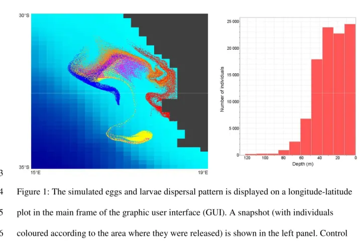
Ichthyop offers two functioning modes. The first one allows a visualization of the transport of 23
virtual eggs and larvae in a user-friendly graphic interface (Figure 1). The second mode 24
enables to run series of simulations based on pre-defined sets of parameters, with a minimalist 1 interface. 2 3 Figure 1 4 5
The tool is a generic version of previous modelling experiments investigating the effects of 6
physical and biological factors on the dynamics of anchovy and sardine ichthyoplankton in 7
the Benguela (Mullon et al. 2002, Huggett et al. 2003, Mullon et al. 2003, Parada et al. 2003, 8
Lett et al. 2006, Miller et al. 2006, Lett et al. 2007b) and in the Humboldt (Lett et al. 2007a, 9
Brochier et al. submitted) upwelling systems. 10
11
The model
12 13
The model description follows the Overview-Design-Details (ODD) protocol for describing 14
individual- and agent-based models (Grimm et al. 2006) and consists of seven elements. The 15
first three elements provide an overview, the fourth element explains general concepts 16
underlying the model’s design, and the remaining three elements provide details. 17
18
Purpose
19 20
Ichthyop is an individual-based model (IBM) designed to study the effects of physical and 21
biological factors on the dynamics of fish eggs and larvae. 22
23
State variables and scales
The IBM comprises individuals and their physical environment. Individuals are characterized 1
by the state variables: age [day], length [mm], stage (egg, yolk-sac larva or feeding larva), 2
location (longitude [°E], latitude [°N] and depth [m]) and status (alive or dead). The physical 3
environment is characterized by ocean state variables: current velocities [m.s-1], temperature 4
[°C] and salinity. 5
6
The environment state variables are provided on a discrete three-dimensional grid by archived 7
simulations of the ROMS or MARS oceanic models. As an example of typical spatial scales 8
used to characterize the environment, we describe the ROMS southern Benguela 9
configuration grid (Penven et al. 2001) It extends from 28 to 40° S and from 10 to 24° E. The 10
horizontal resolution ranges from 9 km at the coast to 16 km offshore. The vertical resolution 11
ranges from 1 to 4.7 m at the surface and from 3.1 to 1030 m at the bottom of the ocean. 12
13
The IBM sees the Eulerian velocity field at the same spatial scale as the Eulerian primitive 14
equation models (ROMS/MARS). Subgriscale parameterizations can be added in the IBM to 15
address scales unresolved by the primitive equation models (see the dispersion terms in the 16
IBM movement submodel below). 17
18
In ROMS, the current velocities, temperature and salinity fields are typically averaged over 19
time and stored every day or so. In the IBM, these fields are interpolated in space to provide 20
values at any individual location. They are also interpolated in time to feed the IBM time step 21
(typically one hour). Simulations consist in tracking the locations and properties of the 22
individuals (typically during a few weeks or months). 23
24
Process overview and scheduling
After initialization (spawning), the IBM proceeds in discrete time steps. Within each time step 1
each individual moves, grows and tests for mortality and recruitment. The spawning, 2
movement, growth, mortality and recruitment submodels are described below. The 3
environment state variables are updated during the simulation at a frequency equal to that of 4
the ROMS/MARS stored outputs. 5
6
Design concepts
7 8
Stochasticity. The release location of each individual is chosen randomly within the specified
9
spawning areas. This is used to simulate patchy or uniform distributions depending on a 10
patchiness parameter (see the spawning submodel below). The horizontal and vertical 11
dispersion components of the movement (see the movement submodel below) are also 12
stochastic. 13
14
Observation. The advection part of the movement submodel has been tested by recording
15
trajectories of individuals and comparing them to trajectories obtained using two other 16
Lagrangian tools (“Roff”, Capet et al. 2004, Carr et al. 2008, 17
http://www.atmos.ucla.edu/~capet/Myresearch/my_research_floats.html; “Ariane”, Blanke 18
and Raynaud 1997, Blanke et al. 1999, http://www.univ-brest.fr/lpo/ariane). The present tool 19
offers two functioning modes (a graphic interface and a serial mode, see “The tool” section 20
above) and associated observation modes (output files, see “The simulations” section below). 21
22
Initialization
23 24
The IBM first loads a configuration file (see “The simulations” section below). Then 1
individuals are released according to a spawning strategy set by the user (see the spawning 2
submodel below), at the egg stage, with an initial length of 0.025 mm. 3
4
Input
5 6
The fields of environment state variables are the input of the IBM. They are provided by 7
archived simulations of ROMS or MARS. 8
9
Submodels
10 11
Spawning. The spawning strategy is defined by the user. The tool offers two modes for
12
releasing eggs. The first one, zone release, implies setting the number of eggs and the 13
spawning areas, depth, frequency and patchiness. Each spawning area is defined by the 14
coordinates (longitude [°E], latitude [°N]) of four points and by two bathymetric lines [m]. 15
The four points delimit a polygon and the spawning area is set as the portion of the polygon 16
contained between the bathymetric lines. Depth of spawning is defined by upper and lower 17
depth levels [m]. Spawning begins at the beginning of the simulation. There may be several 18
spawning events: the number of spawning events and the time between two events are set by 19
the user. Eggs may be released by patches inside the spawning areas: the user defines the 20
number of patches, their radius (horizontal dimension [m]) and thickness (vertical dimension 21
[m]). The alternative release mode allows reading the initial location of the released 22
individuals from input files (see the Ichthyop user guide). 23
Movement. The movement submodel simulates the following processes: horizontal advection,
1
vertical advection, horizontal dispersion, vertical dispersion, egg buoyancy and larval vertical 2
migration. Horizontal advection is always used in the movement equation. Vertical advection 3
is always used too, except at the larval stage if the user chooses to apply the vertical migration 4
scheme instead. The vertical migration scheme implemented is diel vertical migration where 5
larvae spend daytime and night-time at user-specified depths. Daytime begins at 7 a.m. and 6
night-time at 7 p.m. A user who wants to change these values or to consider another vertical 7
migration scheme will have to make changes in this submodel (see the Ichthyop user guide). 8
The user can choose to apply a buoyancy scheme at the egg stage. When buoyancy is taken 9
into account a term is added to the vertical velocity. This term depends on the difference 10
between egg density and water density. Egg density [g.cm-3] is a parameter chosen by the user 11
and water density is a function of temperature and salinity. For a complete description of the 12
buoyancy scheme we refer to Parada et al. (2003). The user can also choose to apply 13
horizontal dispersion and vertical dispersion. Horizontal dispersion has been implemented 14
following Peliz et al. (2007). A random displacement model has been implemented for 15
vertical dispersion (Visser 1997), using a cubic spline interpolation of the vertical diffusivity 16
fields read in the environment state variables. For time-stepping a forward-Euler or a 4th order 17
Runge-Kutta integration schemes can be used. 18
Growth. Length l [mm] increases linearly with time t [day] (eq. 1a), at a rate r taken as a
19
linear function of temperature T [°C] (eq. 1b). 20 21 t r t l t t l( +∆ )= ( )+ ∆ T r=0.02+0.03 (1a) (1b) 22
Individuals change stages according to their length, going from egg to yolk-sac larva at 2.8 1
mm, and from yolk-sac larva to feeding larva at 4.5 mm. These values and equations (1) are 2
used to simulate the growth of anchovy in the southern Benguela upwelling system. A user 3
who wants to consider another species or location may have to make changes in this 4
submodel (see the Ichthyop user guide). 5
6
If plankton concentrations are provided in the environment state variables used in Ichthyop 7
(e.g., they result from simulations of a NPZD biogeochemical model coupled to ROMS, Koné 8
et al. 2005), the user may choose to apply, at the feeding larvae stage, a growth function 9
limited by food (eq. 2): 10 11 ) 03 . 0 02 . 0 ( T Food K Food r s + + = (2) 12
where K is a half saturation constant and Food a function of phytoplankton and zooplankton s
13
concentrations (Koné 2006) that can be specified in the source code. 14
15
Mortality. Individuals die when they are in waters at a temperature below a certain value. This
16
value of lethal temperature [°C] may be different for eggs and for larvae, and is user-17
specified. 18
19
Recruitment. Individuals are considered as recruited when they have reached a minimum
20
length (or age) and spent a minimum amount of time within a “recruitment area”. Recruitment 21
minimum length (or age) at recruitment and the minimum duration of stay within recruitment 1
areas are determined by the user. 2
3
The Simulations
4 5
Simulations are performed using either the graphic interface (SINGLE) mode of the tool or its 6
series of simulations (SERIAL) mode. Which of these two modes is used depends on the 7
value of the “run” field in the configuration file. 8
9
Configuration files. Configuration files enable the user to specify the conditions under which
10
simulations are performed. As part of the Ichthyop tool a configuration editor helps designing 11
configuration files for the SINGLE mode. Configuration files for the SERIAL mode have to 12
be designed using a text editor. Basic examples of SINGLE and SERIAL configuration files 13
are provided in the tool. We refer to the Ichthyop user guide for details about configuration 14
files. 15
16
Output files. Output files are screen snapshots (Figure 1) in the SINGLE mode, and NetCDF
17
files in both SINGLE and SERIAL modes. In the NetCDF output files are recorded the state 18
variables of all individuals and of the environment they experience. We refer to the Ichthyop 19
user guide for details about these output files. They can be post-processed easily using 20
graphic and statistical software. Routines in R (Hornik 2007) for plotting trajectories of 21
individuals or for computing the number of individuals transported from spawning areas to 22
recruitment areas can be sent upon request. 23
Conclusion
1 2
Ichthyop is a tool designed to be shared within the community using models coupling physics 3
with ichthyoplankton dynamics. Though it has been historically developed to study the 4
dynamics of small pelagic fish ichthyoplankton in upwelling systems, Ichthyop is a generic 5
tool in the sense that it incorporates the most important processes involved in ichthyoplankton 6
dynamics. Using Ichthyop for other species in other systems may imply a few changes in the 7
source code (e.g., changing the growth function, implementing a specific larval vertical 8
migration scheme, etc.). This code is organized simply, commented and documented, which 9
should make it easy to modify by a user with basic programming skills. 10
11
Acknowledgements
12 13
We are grateful to PREVIMER for financial support. We also thank Franck Dumas, John 14
Field, Pierre Garreau, Fabrice Lecornu and Claude Roy, and three anonymous reviewers for 15
their helpful comments. 16
References
1 2
Blanke, B., Raynaud, R., 1997. Kinematics of the Pacific Equatorial Undercurrent: an 3
Eulerian and Lagrangian approach from GCM results. Journal of Physical Oceanography 27 4
(6) 1038-1053. 5
6
Blanke, B., Arhan, M., Speich, S., Madec, G., 1999. Warm water paths in the equatorial 7
Atlantic as diagnosed with a general circulation model. Journal of Physical Oceanography 29 8
(11) 2753-2768. 9
10
Capet, X.J., Marchesiello, P., McWilliams, J.C., 2004. Upwelling response to coastal wind 11
profiles. Geophysical Research Letters 31 (13) L13311, doi:10.1029/2004GL020123. 12
13
Carr, S.D., Capet, X.J., McWilliams, J.C., Pennington, J.T., Chavez, F.P., 2008. The influence 14
of diel vertical migration on zooplankton transport and recruitment in an upwelling region: 15
estimates from a coupled behavioral-physical model. Fisheries Oceanography 17 (1) 1-15. 16
17
Gallego, A., North, E.W., Petitgas, P., 2007. Introduction: status and future of modelling 18
physical-biological interactions during the early life of fishes. Marine Ecology-Progress 19
Series 347 121-126. 20
21
Grimm, V., Berger, U., Bastiansen, F., Eliassen, S., Ginot, V. et al. 2006. A standard protocol 22
for describing individual-based and agent-based models. Ecological Modelling 198 (1-2) 115-23
126. 24
Hornik, K., 2007. The R FAQ. http://CRAN.R-project.org/doc/FAQ/R-FAQ.html, ISBN 3-1
900051-08-9. 2
3
Huggett, J., Fréon, P., Mullon, C., Penven, P., 2003. Modelling the transport success of 4
anchovy Engraulis encrasicolus eggs and larvae in the southern Benguela: the effect of 5
spatio-temporal spawning patterns. Marine Ecology Progress Series 250 247-262. 6
7
Koné, V., 2006 (in French). Modélisation de la production primaire et secondaire de 8
l'écosystème du Benguela sud. Influence des conditions trophiques sur le recrutement des 9
larves d'anchois. Ph.D. thesis, Université Paris VI. 10
11
Koné, V., Machu, E., Penven, P., Andersen, V., Garçon, V., Fréon, P., Demarcq, H., 2005. 12
Modeling the primary and secondary productions of the southern Benguela upwelling system: 13
a comparative study through two biogeochemical models. Global Biogeochemical Cycles 19 14
(4) GB4021, doi:4010.1029/2004GB002427. 15
16
Lazure, P., Dumas, F., 2008. An external-internal mode coupling for a 3D hydrodynamical 17
model for applications at regional scale (MARS). Advances in Water Resources 31 233-250. 18
19
Lett, C., Roy, C., Levasseur, A., van der Lingen, C.D., Mullon, C., 2006. Simulation and 20
quantification of enrichment and retention processes in the southern Benguela upwelling 21
ecosystem. Fisheries Oceanography 15 (5) 363-372. 22
23
Lett, C., Penven, P., Ayón, P., Fréon, P., 2007a. Enrichment, concentration and retention 24
processes in relation to anchovy (Engraulis ringens) eggs and larvae distributions in the 25
1
Lett, C., Veitch, J., van der Lingen, C.D., Hutchings, L., 2007b. Assessment of an 2
environmental barrier to transport of ichthyoplankton from the southern to the northern 3
Benguela ecosystems. Marine Ecology Progress Series 347 247-259. 4
5
Miller, D.C.M., Moloney, C.L., van der Lingen, C.D., Lett, C., Mullon, C., Field, J.G., 2006. 6
Modelling the effects of physical-biological interactions and spatial variability in spawning 7
and nursery areas on transport and retention of sardine eggs and larvae in the southern 8
Benguela ecosystem. Journal of Marine Systems 61 (3-4) 212-229. 9
10
Miller, T.J., 2007. Contribution of individual-based coupled physical biological models to 11
understanding recruitment in marine fish populations. Marine Ecology-Progress Series 347 12
127-138. 13
14
Mullon, C., Cury, P., Penven, P., 2002. Evolutionary individual-based model for the 15
recruitment of anchovy (Engraulis capensis) in the southern Benguela. Canadian Journal of 16
Fisheries and Aquatic Sciences 59 (5) 910-922. 17
18
Mullon, C., Fréon, P., Parada, C., van der Lingen, C., Huggett, J., 2003. From particles to 19
individuals: modelling the early stages of anchovy (Engraulis capensis/encrasicolus) in the 20
southern Benguela. Fisheries Oceanography 12 (4-5) 396-406. 21
22
Parada, C., van der Lingen, C.D., Mullon, C., Penven, P., 2003. Modelling the effect of 23
buoyancy on the transport of anchovy (Engraulis capensis) eggs from spawning to nursery 24
1
Peliz, A., Marchesiello, P., Dubert, J., Marta-Almeida, M., Roy, C., Queiroga, H., 2007. A 2
study of crab larvae dispersal on the Western Iberian Shelf: physical processes. Journal of 3
Marine Systems 68 215-236. 4
5
Penven, P., Roy, C., Brundrit, G.B., Colin de Verdière, A., Fréon, P., Johnson, A.S., 6
Lutjeharms, J.R.E., Shillington, F.A., 2001. A regional hydrodynamic model of upwelling in 7
the Southern Benguela. South African Journal of Science 97 (11-12) 472-475. 8
9
Shchepetkin, A.F., McWilliams, J.C., 2005. The regional oceanic modeling system (ROMS): 10
a split-explicit, free-surface, topography-following-coordinate oceanic model. Ocean 11
Modelling 9 (4) 347-404. 12
13
Visser, A.W., 1997. Using random walk models to simulate the vertical distribution of 14
particles in a turbulent water column. Marine Ecology-Progress Series 158 275-281. 15
Figures
1 2
3
Figure 1: The simulated eggs and larvae dispersal pattern is displayed on a longitude-latitude 4
plot in the main frame of the graphic user interface (GUI). A snapshot (with individuals 5
coloured according to the area where they were released) is shown in the left panel. Control 6
graphs, like the one in the right panel (showing the depth distribution of individuals), can be 7
added in the GUI. 8