Transient energy growth of optimal streaks in parallel round jets
Texte intégral
Figure
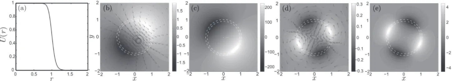
![FIG. 7. Transient dynamics of optimal perturbations with m = 2 (top row) and m = 10 (bottom row) for frozen base flows at Re = 100 000: [(a) and (e)] normalized axial components of enstrophy density | ! z (r ) | 2 / max( | ! z (r ) | 2 ) at t = 0 and [(b)](https://thumb-eu.123doks.com/thumbv2/123doknet/14354265.501483/10.892.86.806.130.490/transient-dynamics-optimal-perturbations-normalized-components-enstrophy-density.webp)

![FIG. 11. Transient dynamics of perturbations for a diffusing base flow with ↵ = 20 and Re = 1000: cross section of the optimal initial condition (t = 0) axial vorticity ! z and associated normalized vector field [(c) and (g)] and streamwise velocity u z of](https://thumb-eu.123doks.com/thumbv2/123doknet/14354265.501483/12.892.85.805.712.1072/transient-perturbations-diffusing-condition-vorticity-associated-normalized-streamwise.webp)
![FIG. 12. Energy density distributions for optimal perturbations with m = 1 [(a)-(f)] and m = 2 [(g)-(l)] for diffusive (top row) and frozen (bottom row) base flows with ↵ = 20 at Re = 1000: radial energy densities |u i (r)| 2 at (a), (d), (g), and (j) init](https://thumb-eu.123doks.com/thumbv2/123doknet/14354265.501483/13.892.84.807.129.407/energy-density-distributions-optimal-perturbations-diffusive-frozen-densities.webp)


Documents relatifs
La décentralisation est un phénomène relié au transfert de pouvoir des organes de décision de l’état central œuvrant dans la capitale vers soit des organes de l’état central
Since 2004, the wooden panel of the “Mona Lisa” painting by Leonardo da Vinci has been studied by an international research group of scientists [1,2] and several experimental
33 (a) Institute of High Energy Physics, Chinese Academy of Sciences, Beijing; (b) Department of Modern Physics, University of Science and Technology of China, Anhui; (c) Department
Les mineurs étrangers et les “deuxièmes générations” sont perçus en Italie — mais probablement aussi dans d’autres contextes nationaux — comme une réalité qui dépasse
In a sense, an adapted (best) basis Next section gives a brief review of noise removal serhisitmteyte.l(or signal en- .by thresholding and of wavepacket
/ La version de cette publication peut être l’une des suivantes : la version prépublication de l’auteur, la version acceptée du manuscrit ou la version de l’éditeur. Access
method to prepare the organoclay/epoxy nanocomposites in liquid (ethanol and water solution) without any intermediate drying step of clay has been used but full exfoliation still
5.24 – Estimation du CRC pour la grosse sph` ere en fonction du bruit pr´ esent dans les donn´ ees reconstruites pour la reconstruction des projections
