HAL Id: hal-02025696
https://hal.archives-ouvertes.fr/hal-02025696
Submitted on 19 Feb 2019
HAL is a multi-disciplinary open access
archive for the deposit and dissemination of
sci-entific research documents, whether they are
pub-lished or not. The documents may come from
teaching and research institutions in France or
abroad, or from public or private research centers.
L’archive ouverte pluridisciplinaire HAL, est
destinée au dépôt et à la diffusion de documents
scientifiques de niveau recherche, publiés ou non,
émanant des établissements d’enseignement et de
recherche français ou étrangers, des laboratoires
publics ou privés.
Victor Sofonea
To cite this version:
Benjamin Piaud, Stéphane Blanco, Richard Fournier, Victor Eugen AmbruŞ, Victor Sofonea.
GAUSS QUADRATURES-THE KEYSTONE OF LATTICE BOLTZMANN MODELS.
Interna-tional Journal of Modern Physics C, World Scientific Publishing, 2014, 25 (01), pp.1340016.
�10.1142/S0129183113400160�. �hal-02025696�
c
World Scientific Publishing Company
GAUSS QUADRATURES – THE KEYSTONE OF LATTICE BOLTZMANN MODELS
BENJAMIN PIAUD
HPC – SA, 3 Chemin du Pigeonnier de la Cepi`ere, F – 31100 Toulouse, France benjamin.piaud@hpc-sa.com
ST ´EPHANE BLANCO, RICHARD FOURNIER
Universit´e de Toulouse, UPS, INPT; UMR 5213 LAPLACE / GREPHE 118 Route de Narbonne, F – 31062 Toulouse Cedex 9, France stephane.blanco@laplace.univ-tlse.fr, richard.fournier@laplace.univ-tlse.fr
VICTOR EUGEN AMBRUS¸, VICTOR SOFONEA∗
Center for Fundamental and Advanced Technical Research, Romanian Academy Bd. Mihai Viteazul 24, RO - 300223 Timi¸soara, Romania
victor.ambrus@gmail.com, sofonea@acad-tim.tm.edu.ro
Received Day Month Year Revised Day Month Year
In this paper we compare two families of Lattice-Boltzmann models derived by means of Gauss quadratures in the momentum space. The first one is the HLB(N; Qx, Qy, Qz) family, derived by using the Cartesian coordinate system and the Gauss-Hermite quadra-ture. The second one is the SLB(N; K, L, M) family, derived by using the spherical coordi-nate system and the Gauss-Laguerre, as well as the Gauss-Legendre quadratures. These models order themselves according to the maximum order N of the moments of the equilibrium distribution function that are exactly recovered. Microfluidics effects (slip velocity, temperature jump, as well as the longitudinal heat flux that is not driven by a temperature gradient) are accurately captured during the simulation of Couette flow for Knudsen number up to 0.25.
Keywords: Lattice Boltzmann; Gauss quadrature; microfluidics; Couette flow PACS Nos.: 47.11.-j, 47.61.-k, 51.10.+y
1. Introduction
In their early days, the Lattice Boltzmann (LB) models were designed to retrieve the Navier-Stokes equation in the incompressible limit by using a discrete set of vectors
in the two- (2D) or three-dimensional (3D) momentum space.1,2,3,4,5 More
conve-nient LB models (isothermal or with variable temperature) were derived later using ∗Corresponding author.
2 B. Piaud, S. Blanco, R. Fournier, V. E. Ambru¸s & V. Sofonea
the Gauss-Hermite quadrature.6,7,8,9Such models form a hierarchy and higher order
moments of the equilibrium distribution functions are successively achieved when
increasing the position of an LB model in the hierarchy.10,11,12 This is particularly
important when approaching microfluidics problems.13,14,15,16,17,18
In this paper, we briefly outline the basics of the derivation of three-dimensional (3D) LB models based on Gauss quadratures. There are two families of such models, which differ by the coordinate system (Cartesian of spherical) used in the momen-tum space and we consider the thermal Couette flow problem to compare the results obtained by using both models.
2. Lattice Boltzmann models derived by Gauss quadratures
Let us consider the equilibrium distribution function feq ≡ feq(p; n, u, T ) =
n(β/π)D/2e−β(p−mu)2
, where p is the momentum vector (whose Cartesian
com-ponents in the D-dimensional space are pα, 1 ≤ α ≤ D), m is the mass of the fluid
particles, n is the local particle number density, u is the local fluid velocity, T is the local fluid temperature and β = 1/2mT . According to the Chapman-Enskog method, the derivation of the conservation equations from the Boltzmann equation involves the calculation of the moments of the distribution functions up to a certain order S (0 ≤ s ≤ S): M(s){αl}≡ M(s) α1α2...αs = Z dDpfeq s Y l=1 pαl (1 ≤ αl≤ D) (1)
In the LB models, the integral in the equation above is replaced by summation over
a discrete set of momentum vectors {pi∈I}, where I is an index set. Accordingly,
the equilibrium distribution function f(eq) is replaced by the set of distribution
functions fieq≡ winEN(pi; u, T ), i ∈ I, where EN(p; u, T ) is a polynomial of order
N with respect to p. After these replacements, Eq. (1) becomes:
f M(s){α l}≡ fM (s) α1α2...αs = X i∈I fieq s Y l=1 piαl (2)
In practice, EN(p; u, T ) might be expanded with respect to some orthogonal
poly-nomials set, e.g., Hermite polypoly-nomials.6,7,8,9,19,20,21 This allows one to determine
the momentum vectors pi, as well as their associated weights wi (i ∈ I) by using
appropriate Gauss quadratures21that ensure M(s){α
l}= fM (s)
{αl}for 0 ≤ s ≤ S.
7,8,18,20
As stated in Refs. 19 and 20, the condition N ≥ S needs to be satisfied in other to retain all relevant moments up to order S.
The integration over the whole momentum space, which appears in Eq. (1), may be performed in using the separation of variables along the axes of the coordinate system. When D = 3, both the Cartesian and the spherical coordinate systems may be used for this purpose. In the first case, the equilibrium distribution function is
expansion involving the generalized Laguerre polynomials, as well as the Legendre
polynomials, is used in the second case.18,22
In principle, the Gauss quadrature method allows one to build LB models of order N as large as needed by using appropriate momentum vector sets. The num-ber of the vectors is determined by the quadrature order(s) and the projections of these vectors on the axes of the coordinate system are related to the roots of
or-thogonal polynomials.7,8,9,10,18,19,20 This feature greatly facilitates the assembling
of LB models of any order and LB models with momentum sets up to 8,000 ele-ments, which run successfully on high performance computing systems, were already
reported.17,18,23Although the number of momentum vectors in the set becomes very
large when increasing N , it can be reduced by pruning techniques at the cost of sacrificing the accuracy of some higher-order moments of the distribution function
or by taking advantage of the symmetry group of the lattice.11,15,24 However, such
techniques are very elaborated and need to be carefully designed for each N .
In the sequel, we will denote by HLB(N ; Qx, Qy, Qz) the 3D LB model of
or-der N based on Gauss-Hermite quadratures, where Ql is the order of the
quadra-ture used along the l axis (1 ≤ l ≤ 3). The spherical LB models are denoted by SLB(N ; K, L, M ), where K, L, M are the orders of the quadratures with respect
to the spherical coordinates r, θ and φ, respectively.18,22 Since both models are
off-lattice, a flux limiter numerical scheme17,18,25 involving the projection of the
discrete momenta on the Cartesian axes was used to compute the evolution of the
distribution functions after each time step. The Shakhov collision term18,26,27,28was
used in these models to achieve the right value (2/3) of the Prandtl number.
3. Computer results
To compare the characteristics of the two families of quadrature-based LB models (HLB and SLB), we considered the problem of thermal Couette flow between two
parallel plates perpendicular to the z axis. The plates are located at zb= −0.5 and
zt= 0.5, respectively and move in opposite directions along the y axis with speed
uw = 0.63. Their temperatures is T = 1.0 (nondimensionalized units18 are used).
The computer simulations were done on a cubic lattice with 128 nodes in the z direction and 2 nodes in the x and y direction. Periodic boundary conditions were
applied along the x and y axes and the diffuse reflection boundary conditions17,18,29
were applied on the plates. The results reported in this paper were obtained with
the lattice spacing δs = 1/128 and the time step δt = 10−4.
Figure 1 shows the transversal profiles of the longitudinal velocity uy, the
tem-perature T , the transversal heat flux qz, as well as the longitudinal heat flux qy.
These profiles were obtained in the stationary state with the Shakhov collision term by using the models HLB(6;20,20,20) and SLB(6;20,20,20), for three values of the Knudsen number. The profiles are compared to the Direct Simulation Monte Carlo (DSMC) results for hard sphere molecules reported in Refs. 30 and 31. We used the
4 B. Piaud, S. Blanco, R. Fournier, V. E. Ambru¸s & V. Sofonea -0.6 -0.4 -0.2 0 0.2 0.4 0.6 -0.5 -0.25 0 0.25 0.5 fluid velocity u y z coordinate DSMC Kn = 0.01 DSMC Kn = 0.10 DSMC Kn = 0.25 HLB Kn = 0.01 HLB Kn = 0.10 HLB Kn = 0.25 SLB Kn = 0.01 SLB Kn = 0.10 SLB Kn = 0.25 1 1.02 1.04 1.06 1.08 1.1 -0.5 -0.25 0 0.25 0.5 fluid temperature T z coordinate DSMC Kn = 0.01 DSMC Kn = 0.10 DSMC Kn = 0.25 HLB Kn = 0.01 HLB Kn = 0.10 HLB Kn = 0.25 SLB Kn = 0.01 SLB Kn = 0.10 SLB Kn = 0.25 -0.09 -0.06 -0.03 0 0.03 0.06 0.09 -0.5 -0.25 0 0.25 0.5
transversal heat flux q
z z coordinate DSMC Kn = 0.01 DSMC Kn = 0.10 DSMC Kn = 0.25 HLB Kn = 0.01 HLB Kn = 0.10 HLB Kn = 0.25 SLB Kn = 0.01 SLB Kn = 0.10 SLB Kn = 0.25 -0.08 -0.06 -0.04 -0.02 0 0.02 0.04 0.06 0.08 -0.5 -0.25 0 0.25 0.5
longitudinal heat flux q
y z coordinate DSMC Kn = 0.01 DSMC Kn = 0.10 DSMC Kn = 0.25 HLB Kn = 0.01 HLB Kn = 0.10 HLB Kn = 0.25 SLB Kn = 0.01 SLB Kn = 0.10 SLB Kn = 0.25
Fig. 1. Velocity, temperature and heat flux profiles in Couette flow obtained with models HLB(6;20,20,20) and SLB(6;20,20,20 at three values of the Knudsen number Kn.
Good agreement between the LB and DSMC results is observed for all quantities,
excepting the temperature results at Kn = 0.25.18The specific microfluidics effects
(slip velocity, temperature jump, as well as the longitudinal heat flux that is not driven by a temperature gradient) are accurately captured.
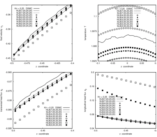
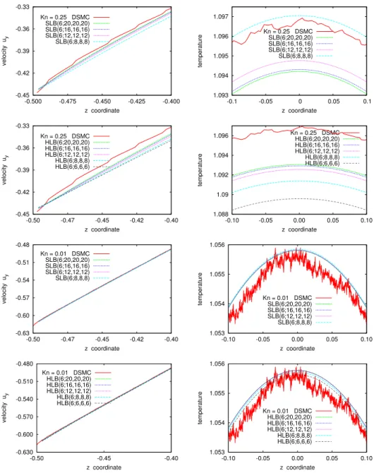
According to Figure 2, the HLB(N;20,20,20) and SLB(N;20,20,20) results get well superposed for N ≥ 4 and N ≥ 3, respectively. As seen in Figure 3, both the HLB and the SLB models are found to be very sensible with respect to the quadra-ture orders when the Knudsen number is large enough. This behavior originates from the half-space integrals involved in the implementation of the diffuse reflec-tion boundary condireflec-tions. As menreflec-tioned in the literature, the errors are reduced and the simulation results converge when the quadrature orders (i.e., the number
-0.45 -0.42 -0.39 -0.36 -0.5 -0.475 -0.45 -0.425 -0.4 fluid velocity u y z coordinate Kn = 0.25 DSMC HLB(7;20,20,20) SLB(7;20,20,20) HLB(4;20,20,20) SLB(4;20,20,20) HLB(3;20,20,20) SLB(3;20,20,20) HLB(2;20,20,20) SLB(2;20,20,20) 1.0925 1.095 1.0975 1.1 -0.1 -0.05 0 0.05 0.1 temperature T z coordinate Kn = 0.25 DSMC HLB(7;20,20,20) SLB(7;20,20,20) HLB(4;20,20,20) SLB(4;20,20,20) HLB(3;20,20,20) SLB(3;20,20,20) HLB(2;20,20,20) SLB(2;20,20,20) -0.095 -0.09 -0.085 -0.08 -0.075 -0.07 -0.065 -0.5 -0.45 -0.4
transversal heat flux q
z z coordinate Kn = 0.25 DSMC HLB(7;20,20,20) SLB(7;20,20,20) HLB(4;20,20,20) SLB(4;20,20,20) HLB(3;20,20,20) SLB(3;20,20,20) HLB(2;20,20,20) SLB(2;20,20,20) 0.04 0.08 0.12 0.16 0.2 -0.5 -0.45 -0.4
longitudinal heat flux q
y z coordinate Kn = 0.25 DSMC HLB(7;20,20,20) SLB(7;20,20,20) HLB(4;20,20,20) SLB(4;20,20,20) HLB(3;20,20,20) SLB(3;20,20,20) HLB(2;20,20,20) SLB(2;20,20,20)
Fig. 2. Velocity and heat flux profiles near the left wall, as well as temperature profiles in the central region of Couette flow at Kn = 0.25, for various values of N .
4. Conclusion
In this paper we compared the simulation results obtained by using two families of LB models based on Gauss quadratures. When using the Shakhov collision term, both families of LB models allows one to accurately capture microfluidics effects (slip velocity, temperature jump, as well as the longitudinal heat flux that is not driven by a temperature gradient) in Couette flow when Kn < 0.25. The main advantage of these models is that the momentum vector sets can be easily constructed, regardless of the order N of the model. This feature is particularly helpful for the accurate implementation of the diffuse reflection boundary conditions, which needs large momentum sets as Kn increases.
Acknowledgments
This work was initiated during the visits of VS to Toulouse (2009 and 2010, sup-ported by CNRS). Support by CNCSIS-UEFISCSU projects PNII-IDEI ID 76/2010 and PN-II-ID-PCE-2011-3-0516 is acknowledged by authors VEA and VS. The
au-6 B. Piaud, S. Blanco, R. Fournier, V. E. Ambru¸s & V. Sofonea -0.45 -0.42 -0.39 -0.36 -0.33 -0.500 -0.475 -0.450 -0.425 -0.400 velocity u y z coordinate Kn = 0.25 DSMC SLB(6;20,20,20) SLB(6;16,16,16) SLB(6;12,12,12) SLB(6;8,8,8) 1.093 1.094 1.095 1.096 1.097 -0.1 -0.05 0 0.05 0.1 temperature z coordinate Kn = 0.25 DSMC SLB(6;20,20,20) SLB(6;16,16,16) SLB(6;12,12,12) SLB(6;8,8,8) -0.45 -0.42 -0.39 -0.36 -0.33 -0.50 -0.47 -0.45 -0.42 -0.40 velocity u y z coordinate Kn = 0.25 DSMC HLB(6;20,20,20) HLB(6;16,16,16) HLB(6;12,12,12) HLB(6;8,8,8) HLB(6;6,6,6) 1.088 1.09 1.092 1.094 1.096 -0.10 -0.05 0.00 0.05 0.10 temperature z coordinate Kn = 0.25 DSMC HLB(6;20,20,20) HLB(6;16,16,16) HLB(6;12,12,12) HLB(6;8,8,8) HLB(6;6,6,6) -0.63 -0.60 -0.57 -0.54 -0.51 -0.48 -0.50 -0.47 -0.45 -0.42 -0.40 velocity u y z coordinate Kn = 0.01 DSMC SLB(6;20,20,20) SLB(6;16,16,16) SLB(6;12,12,12) SLB(6;8,8,8) 1.053 1.054 1.055 1.056 -0.10 -0.05 0.00 0.05 0.10 temperature z coordinate Kn = 0.01 DSMC SLB(6;20,20,20) SLB(6;16,16,16) SLB(6;12,12,12) SLB(6;8,8,8) -0.630 -0.600 -0.570 -0.540 -0.510 -0.480 -0.50 -0.45 -0.40 velocity u y z coordinate Kn = 0.01 DSMC HLB(6;20,20,20) HLB(6;16,16,16) HLB(6;12,12,12) HLB(6;8,8,8) HLB(6;6,6,6) 1.053 1.054 1.055 1.056 -0.10 -0.05 0.00 0.05 0.10 temperature z coordinate Kn = 0.01 DSMC HLB(6;20,20,20) HLB(6;16,16,16) HLB(6;12,12,12) HLB(6;8,8,8) HLB(6;6,6,6)
Fig. 3. Velocity profile parallel to the velocity of the walls (left) and temperature profile (right) at Kn = 0.25 (rows 1 and 2) and Kn = 0.01 (rows 3 and 4) in the SLB (rows 1 and 3) and HLB (rows 2 and 4) models, compared with DSMC results.
thors are grateful to Professor Henning Struchtrup (Department of Mechanical
En-gineering, University of Victoria, Canada) for the DSMC simulation results30,31
system at the West University of Timi¸soara (Romania) using the Portable Exten-sible Toolkit for Scientific Computation (PETSc) developed at Argonne National
Laboratory, Argonne, Illinois.34
References
1. Y. H. Qian, D. d’Humi`eres and P. Lallemand, Europhys. Lett. 17, 479 (1992).
2. H. Chen, S. Chen and W. H. Matthaeus, Phys. Rev. A 45, R5339 (1992). 3. S. Chen and G. D. Doolen, Annu. Rev. Fluid Mech. 30, 329 (1998).
4. S. Succi, The Lattice Boltzmann Equation for Fluid Dynamics and Beyond (Clarendon Press, Oxford, 2001).
5. C. K. Aidun and J. R. Clausen, Annu. Rev. Fluid Mech. 42, 439 (2010). 6. T. Abe, J. Comput. Phys. 131. 241 (1997).
7. X. Y. He and L. S. Luo, Phys. Rev. E 56, 6811 (1997). 8. X. W. Shan and X. Y. He, Phys. Rev. Lett. 80, 65 (1998).
9. S.Ansumali, I. V. Karlin and H. C. ¨Ottinger, Europhys. Lett. 63, 798 (2003).
10. P. C. Philippi, L. A. Hegele, L. O. E. dos Santos and R. Surmas, Phys. Rev. E 73, 056702 (2006).
11. S. S. Chikatamarla and I. V. Karlin, Phys. Rev. E 79, 046701 (2009). 12. X. Shan, Phys. Rev. E 81, 036701 (2010).
13. S. H. Kim, H. Pitsch and I. S. Boyd, J. Comput. Phys. 227, 8655 (2008).
14. W. P. Yudistiawan, S. Ansumali and I. V. Karlin, Phys. Rev. E 78, 016705 (2008). 15. W. P. Yudistiawan, S. K. Kwak, D. V. Patil and S. Ansumali, Phys. Rev. E 82, 046701
(2010).
16. J. P. Meng and Y. H Zhang, J. Comput. Phys. 230, 835 (2011). 17. J. P. Meng and Y. H. Zhang, Phys. Rev. E 83, 036704 (2011). 18. V. E. Ambru¸s and V. Sofonea, Phys. Rev. E 86, 016708 (2012). 19. H. D. Chen and X. W. Shan, Physica D 237, 2003 (2008).
20. X. W. Shan, X. F. Yuan and H. D. Chen, J. Fluid Mech. 550, 413 (2006).
21. F. B. Hildebrand, Introduction to Numerical Analysis (Second Edition, Dover Publi-cations, Inc., New York, 1974).
22. P. Romatschke, M. Mendoza and S. Succi, Phys. Rev. C 84, 034903 (2011).
23. V. Sofonea, B. Piaud, S. Blanco and R. Fournier, Proceedings of the 2nd European Conference on Microfluidics, December 8 – 10, 2010, Toulouse, France (on CD-ROM). 24. J. W. Shim and R. Gatignol, Phys. Rev. E 83, 046710 (2011).
25. J. P. Meng and Y. H. Zhang, Phys. Rev. E 83, 046701 (2011). 26. E. M. Shakhov, Fluid. Dyn. 3, 95 (1968).
27. V. A. Titarev, Comput. Fluids 36, 1446 (2007).
28. I. A. Graur and A. P. Polikaropv, Heat Mass Transf. 46, 237 (2009). 29. S. Ansumali and I. V. Karlin, Phys. Rev. E 66, 026311 (2002). 30. M. Torrilhon and H. Struchtrup, J. Comput. Phys. 227, 1982 (2008).
31. A. Schuetze, Direct Simulation by Monte Calo Modeling Couette Flow using dsmc1as.f: A User’s Manual, Department of Mechanical Engineering, University of Victoria, Canada, 2003 (unpublished).
32. M. Watari, J. Fluids Eng. 132, 101401 (2010).
33. Y. Shi, P. L. Brookes, Y. W. Yap and J. E. Sader, Phys. Rev. E 83, 045701 (2011). 34. S. Balay, K. Buschelman, V. Eijkhout, W. Gropp, D. Kaushik, M. Knepley, L. Curfman
McInnes, B. Smith and H. Zhang, PETSc Users Manual, Argonne National Laboratory Technical Report ANL - 95 /11 - Revision 3.1, 2010 (http://www.mcs.anl.gov/petsc).