A closed-loop otolith system assessment procedure

ASSESSMENT PROCEDURE

By

Dale W. Hiltner

B.S., The Ohio State University, 1978

Submitted in Partial Fulfillment

of the Requirements for the

Degree of Master of Science

at the

Massachusetts Institute of Technology

January, 1983

EJ

Massachusetts Institute of Technology, 1983

Signature of Author

Certified by

Accepted by

Departmegt oferonalics and Astronautics

January 13, 1983

Prof/iau

.xlce

R./YoungA Thesis Supervisor

Chairman, Deparoental Graduate Committee

Professor-Harol Y. Wachman

Aero

&'ASSAC'd SErT R437;TAE

OF TECHNOLOGY

FER

1

0

1'j

MITLibraries

Document Services

Room 14-0551 77 Massachusetts Avenue Cambridge, MA 02139 Ph: 617.253.2800 Email: docs@mit.edu http://Iibraries.mit.edu/docs

DISCLAIMER OF QUALITY

Due to the condition of the original material, there are unavoidable

flaws in this reproduction. We have made every effort possible to

provide you with the best copy available. If you are dissatisfied with

this product and find it unusable, please contact Document Services as

soon as possible.

2

A Closed-Loop Otolith System

Assessment Procedure

by

Dale William Hiltner

Submitted to the Department of Aeronautics and Astronautics

on 13 January 1983 in partial fulfillment of the

requirements for the Degree of Master of Science in

Aeronautics and Astronautics

ABSTRACT

A test procedure that is sensitive to changes in the response of the human otolith system to linear accelerations has been developed. The test

is a closed-loop test in which blindfolded subjects are given a sum of

sinusoids velocity disturbance in the lateral direction and directed to null their subjective velocity using a joystick controller. The test procedure has been optimized to provide the best possible data for all test

subjects. The testing was performed using the M.I.T. Man-Vehicle Laboratory

Sled facility.

Classical

control theory quasi-linear describing

function analysis is

used to analyze the test data. Frequency spectrum plots of the velocity and

joystick signals, along with velocity and joystick RMS values, are used to

measure the velocity nulling performance of the subject. Bode plots

relating acceleration input to joystick velocity command output give the transfer function of the subject.

The Bode plots of four of the subjects tested show very good agreement. The one sigma deviations and data scatter are as low or lower than that of most human subject testing. A regression analysis was used to develop a

transfer function model, GHO. The model, with the values obtained from one

subject, is

2.02(jw)

GHO

=

(jw

+

1.42)(jw

2 +

2(0.144)(0.540)jw

+

(0.540)2)

This test procedure will be used in the pre-and post-flight testing of

astronauts. Its purpose is to define how humans adapt to weightlessness. The results will help to more fully understand the causes of space motion sickness.

Thesis Supervisor: Dr. Laurence R. Young

Acknowledgements

May the wind always be on your tail and your visibility be unlimited.

I would like to thank Prof. Laurence R. Young, Director of the M.I.T.

Man-Vehicle

Laboratory, for allowing me to work on this project and

providing the necessary funding. Many thanks go to Anthony P. Arrott,

acting Project Manager for the M.I.T. Man-Vehicle Laboratory Sled facility,

whose knowledge and advice were of great help to me in thi-s work. Many

thanks go to Linda

Robeck,

the apprentice for this project, for her help with the detail work. Special thanks go to all of my subjects for there

cooperation and patience. I would also like to thank the members of the

Man-Vehicle Laboratory, who were all supportive of me in this work.

I am especially grateful to the members of the Charles Stark Draper Laboratory Leper Colony, of which I am a full member (357), for their comradery and moral support, and for providing needed attitude adjustment

periods. Finally, to my family and friends, thank-you for standing behind

me.

r

4

TABLE OF CONTENTS

Chapter 1 Introduction 6

Chapter 2 Background 11

2.1 Otolith System Testing for Spacelab 11

2.2 The Otolith System Model 14

2.3 The Closed-Loop Task 16

2.4 Engineering Units . 19

Chapter 3 The Experimental System 21

3.1 The M.I.T. Sled 21

3.1.1 Calibrations 25

3.1.2 The Cart Transfer Function 26

3.2 Sled System Software 27

3.2.1 Disturbance Profile Generation 29

3.2.2 Profile Amplitude Scaling

32

3.2.3 The Digital Joystick Filter 34

3.3 Data Reduction 35

Chapter 4 Test Procedure Development 39

4.1 General Concepts 39

4.2 The DHPR02.PRO Series, Part I, and

High Amplitude Probelms 40

4.2.1 Summary 47

4.3 The DHPRO2.PRO Series, Part II, and

Low Amplitude Problems 48

4.3.1

Summary

59

4.4 The H1PR04.PR0 Series and Profile

5

4.4.1 Profile 01

4.4.2 Profiles #3 and

#6

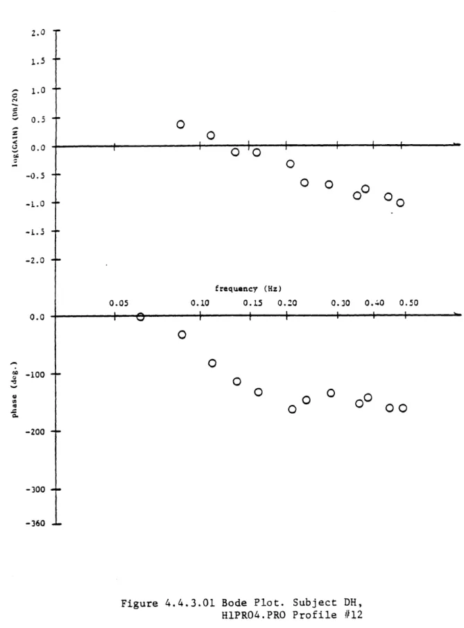
4.4.3 Profile

#12

4.4.4 Summary

4.5

Further Population Testing

4.5.1

Summary

Chapter 5 The Final Experiment

5.1 The Experimental Method

5.2 The Formal Test Procedure

Chapter 6 Results and Discussion

6.1 Results

6.2

Discussion of Individual Subject Results

6.3 The Transfer Function Model

6.4

Remnant Analysis

Chapter 7 Conclusions and Recommendations

7.1 Conclusions

7.2 Recommendations for Further Work

Appendix A: Sled System Pictures

Appendix B: Profile Generation Programs

Appendix C:

Response Analysis Programs

Appendix D: Test Procedure Checklist

D.1 Data Filename Convention Appendix E: Experimental Results

E.1 Plot Format Discussion

References

r

62 71 72 75

78

88

90

90

92

98

98

99

108

115

120

120

123 125 129 146 167 167 175 175 211

L

L.

CHAPTER 1 INTRODUCTION

The purpose of this work is to develop a test procedure that is sensitive

to changes in the response of the human otolith system to linear

accelerations. The test is a closed-loop test in which blindfolded subjects

are given a motion disturbance in the lateral direction and directed to

null their subjective velocity using a joystick controller. This type of

test avoids the magnitude estimation problem of open-loop testing. (Ref. 6)

However, it also involves more non-linear effects caused by the human

operator which will be elaborated upon throughout this work. The

experimental hardware used was the M.I.T. Man-Vehicle Laboratory Sled

facility which is

described in Chapter 3.

The test procedure is

to be used

in pre- and post-flight testing of astronauts. It is expected that the

testing will show changes in the way otolith information is processed by

the brain following exposure to a weightless environment. This information

will then be used to more fully understand space motion sickness.

From previous work with human subjects, Ref. 5,6,7,8, it is known that the acceleration disturbance must not be predictable, as subjects can then

learn the disturbance and respond accordingly. To avoid this a sum of

sinusoids velocity disturbance is used. The current system used on the Sled

has great flexibility in generating these velocity disturbance profiles.

This flexibility involves varying the number of sinusoids, the frequency of

each sinusoid, and the peak magnitude of the velocity or acceleration at

each frequency. Other variables of the system are the gain of the joystick

controller and the pole of the digital filter used to filter this joystick

profile and joystick response by adjusting these parameters.

From

previous work in defining otolith system response, Ref. 4,5,9, it

was found that good response of the otolith system is

obtained in the

0.05-0.5 Hz frequency range. This was the only range considered throughout

the

testing.

The

disturbance

frequencies are determined by

the prime

numbers used to multiply a base frequency. The base frequency is determined

by the desired period. This allows no harmonic multiples to interfere with the disturbance frequencies. The amplitudes of the disturbance 'frequencies can be found using many different techniques. These include defining the

disturbance by a flat position, velocity, or acceleration amplitude, with

or without

scaling by

a

first,

second or third order filter.

This

flexibility was heavily used in developing the final test procedure.

Very little

previous work has been done on otolith testing exclusively.

Meiry in 1965 attempted a closed-loop otolith test but quickly abandoned it

because subjects could not stay within the physical limits of the track.

(Ref. 5) This is because the otolith organs are sensitive to acceleration only, and also have an acceleration threshold of approximately 0.005 g's. Thus, constant velocity motion should be undetectable. These limitations

make the closed-loop task very difficult as will be shown. Also, the works

on human vestibular testing that the author is familiar with do not attempt

to rationalize their disturbance time histories. With no known background

in this specific area of otolith system testing the test procedure had to

be developed from the fundamentals.

Classical control theory describing function techniques are used in the

8

quasi-linear. A block diagram of the system under consideration is shown in

Fig. 1.01. The final criteria for determining if a particular test profile

was acceptable was to look at the frequency response of various signals

obtained

from

the

Sled

system.

The

outputs

available

are

position,

velocity, acceleration,

commanded velocity, and joystick signal. The most

important result is found in the transfer function of the HO which is the

Bode plot relating acceleration input to joystick output. Of secondary

importance, but valuable in qualitative terms, are frequency response plots

of velocity amplitude (with and without HO control) and joystick amplitude.

While the transfer function gives the overall response of the HO, the

amplitude plots give information on individual control differences and

qualitative indications of how well the HO performed the velocity nulling

ta sk.

The development of the final test procedure has proceeded using

experimental techniques. Based on past experience with the Sled some

initial velocity disturbance profiles were generated and tested on several

subjects. Based on this experience new profiles were developed and tested.

Computer simulations were not used in the development phase as most of the

problems discovered in the first tests were non-linear and subjective with

no previously known quantitative definition. Also, the basic model for the

otolith system is linear and would not have shown the non-linear effects

seen. Thus, the final procedure was determined based on actual test data

from all previous tests. Its justification has been by statistical and

qualitative reasoning, rather than by strict mathematical calculations. It

is felt that this gives a fully developed profile, as it is based on actual

velocity

velocity

command cart

ccart

distrbace + to art art accele ration

dynamics

human

joys tick Ioperator,

s ignal .dynamics

10

Thesis Organization

Chapter 2 discusses in more detail the space motion sickness problem and

slows how the test procedure will be utilized. It .also discusses previous

work

involving

the analysis of the human otolith system.

Chapter

3

discusses in detail the M.I.T. Sled facility hardware and software and the

data reduction techniques used. Chapter 4 is a narrative discussion that

reveals the steps taken to achieve the final test procedure. Chapters 5,6,

and 7 discuss the final experimental method, the results, and the significant discoveries of this work.

For those interested in only the method and results, it is suggested that

Chapters 1,5,6, and 7 be read. Those more interested in the full

development process used to obtain the results should read Chapter 2 and 4

also. Those interested in the details of the test facility and the data

BACKGROUND

2.1 Otolith System Testing for Spacelab

This work is part of the Scientific and Technical Proposal for Vestibular

Experiments in Spacelab. (Ref. 1) Its purpose is to define how the human operator changes response to linear accelerations after adapting to

weightlessness. This information will then be used to understand more

fully the causes of

space motion sickness.

A brief description of the

proposal and the scientific background follows.

The first step to achieve this result is to obtain baseline data in the

normal 1 g environment of man. This will be done in the five to six month

period before the Space Shuttle flight STS-9.

Six test

sessions will be

held during this period as shown in Table 2.1.01. The tests will be

conducted on a quick turnaround basis as the astronauts will be available

for only a limited time during each test session. It is also desired for

the test results to be obtained in a reasonable time. Baseline data will be

obtained for each participating astronaut of the STS-9 mission.

Within eight hours of the astronauts return to earth the first

post-flight testing will be done. Subsequent testing will be accomplished over

the next two week period as also seen in Table 2.1.01. This testing will

show how the HO response has changed due to the intervening weightlessness

and will also show a readaptation pattern. In later experiments on the

German 0-1 Spacelab Mission some sled acceleration tests could be performed

12

F0

7

timetable:

Baseline Data Collection

- - - -

-

-18-20 April 1983

28-30 June

21-22 July

31 Aug.-2 September

15-16 September

21-22 September

30 September-8 October

8 October

9-15 October

22-23 October

M.I.T.

Sled

at

U.S.

Lab Sled at

F

=

flight

L

- landing

TABLE 2.1.01

Spacelab

I

Linear Acceleration Sled Test Timetable

M.I.T.

Dryden

"f

F-180

F-90

F-60

F-3

0

F-15

F-8

Flight

L+O

L+1

to

L+l

4

L+7

I I

13

The -- st theory currently available to define the causes of space motion

,ickness is the conflict model theory. (Ref.1,2,3) This theory states that

upon encountering a weightless environment there is a conflict between

'visual, tactile, and semi-circular canal

sensory perception,

and otolith

system sensory perception. This conflict is

caused by the lack of a 1

g

"bias" to the otolith organs. Since the otolith organ output and

corresponding brain interpretation is based on millennia of development in

a 1 g environment this conflict is easily conceptualized. It is felt that

this specific conflict is the cause of space motion sickness.

There are two theories available to explain recovery from space motion

sickness based on the conflict model. The primary theory states that since

without a constant 1 g "bias" acting on the otolith organ the output is

questionable, it

is

inhibited by the brain. More reliance is

then placed on

vision to determine orientation. The HO response to linear acceleration is

therefore not based on the response of the otolith system and otolith

system sensitivity to linear accelerations would be decreased. The

secondary theory states that the brain can cancel the 1 g "bias" effects in

its processing and concentrate on purely linear acceleration. This would

cause an increase in otolith system sensitivity.

These theories must be considered in developing the test

procedure to

measure changes in the response of the otolith system. The procedure must

be able to show an increase or a decrease in otolith system response. The

required performance of the HO must not be maximized or minimized so that

with varying otolith sensitivities the tests can be completed and precise

results obtained.

14

2.2 The Otolith System Model

work in defining the otolith system response is found in Ref. 2. This

1ork

has resulted in the Young and Meiry model shown in Fig.

2.2.01.

,rhe original data for this model was obtained using a system in which the

subject was oscillated at one frequency and indicated the direction of the

motion with a joystick. (Ref. 5) The test was therefore an open-loop process in which only phase information was desired. No amplitude

information was obtained due to the magnitude estimation problem of

open-loop testing. (As stated in Chapter 1, the closed-loop velocity nulling

task was attempted but quickly abandoned due to the inability of subjects

to stay within the track limits for more than 40 seconds). As expected the

Bode plot shows good agreement with the phase data, but the amplitude

information is meaningless. It is this amplitude estimation problem that

the closed-loop task is expected to resolve.

It is noted that this otolith system transfer function is based on a

velocity or acceleration input to the subject and a perceived output

indicated by a hand operated joystick. Thus, it is a model for the complete path from the otolith organ output, through the processing of this

information by the brain which outputs a signal to the muscles of the hand,

and finally to the response of the hand itself.

As such,

this model can

also be used as a basis for the closed-loop task. It is expected that the

response of the subject in the closed-loop task will be similar to this

complete otolith system model.

Possible differences will be discussed in

section 2.3.

15

LATERAL SPECIFIC FOACX 1.5 ( S + 0.0765 1CRCEv(D TtLT AGLI t PERCEIVED

(TILT ANGLE WVRYT. EARTH) (s+0.191 (S+ .31 Oft LATERAL ACCELERATION S LHEAN VELOCITY

CKOUS)RLLN V-LOc1 -e 1 STD 1EVIATIO of 10 'OUmJENCT INAO/sC) to

Figure 2.2.01 The Young & Meiry Model (from Ref. 1)

-I

71, 3 z 11 to 0 *90 -20 * 40 *70p

16

0P-off of the phase at higher frequencies. Assuming the amplitude follows this model it would also show a similar drop-off. This means very little

response

of the HO to disturbances at the high frequencies. To avoid

possible control problems in the closed-loop

task a frequency range of

0.

0 5-0.5Hz was chosen. This allows a full octave range and also contains

the break frequency of 0.22 Hz (1.5 rad/sec) of the model. Good HO response should be obtained over this frequency range and the break

frequency should be indicated to enhance the results.

2.3 The Closed-Loop Task

As stated previously, the main reason for using the closed-loop task is

to resolve the magnitude estimation problem. This hopefully will mean more

correct magnitude response of the subject as well as correspondingly more

correct phase information. However, the closed-loop task contains some

additional effects which must be considered.

A block diagram for the closed-loop task is shown in Fig. 2.3.01. With the subject in the loop as shown, the task is not only motion estimation

but manual control. As in other manual control tasks different control

techniques can be used to achieve the same desired results. This technique,

or control strategy, then becomes a part of the HO response. Also, the HO

is not a linear system and so does not respond only to the disturbance. The

HO will generate some extra response, or remnant, which cannot be linearly

correlated with the disturbance. These aspects of the HO control are

indicated in the block diagram of Fig. 2.3.02. The V=0 summing point

indicates the velocity nulling task. The block diagram shows the complete

HO system, as considered in this work.

vvelocity

velocity + cosmmand cart

disturbance

to cart

cart

acceleration

20

3

dynamics human operator _joys velocity _{siga l} command human joystick operator filter dynamics

Figure 2.3.01 The Closed-Loop

System

cart

velocity velocity cart cr

disturbance command dyamic acceleration

+ +, G (jQ )

human operator

veLocity _remnant

_V-0

_otolith

command _{I+ +}

_control

₊

+ system

filter strategy _dynamics

Gg (jQ) _C 3OW _{G (jw)}

human operator

Figure 2.3,.02 The Closed-Loop Block Diagram

with Details of the Human Operator

L

18

The transfer function for the HO is taken across the human operator block

shown in Fig. 2.3.02. Thus, the transfer function is not that for the

otolith

system obtained by open-loop testing. The purpose of this thesis is

not to define the control strategy transfer function, but its

effects are

important and will be elaborated upon throughout this work. The transfer

function obtained in this thesis will contain the control strategy effects.

This will not effect the desired result, which is to measure HO performance

in the closed-loop task, but will effect the analysis and obseryations of

the data.

Of more minor importance from a scientific standpoint but important in a

practical sense is the limited track length of the Sled. Because the

otolith organs act as accelerometers only, no output will occur for

constant velocity motion. (Ref. 5,9) This will cause difficulties for the HO in the closed-loop task. Without an acceleration input deciding on a

control input will then be accomplished by guessing. Also, as noted in Ref.

4, subjects often indicate the wrong direction of motion in the open-loop

task. For the closed-loop task, then, this could mean initially a wrong

control input, as the HO should sense the wrong direction and correct

himself. This shows that there is ample opportunity for the HO to input

improper control and increase his motion instead of decreasing it. Also,

since the HO cannot exactly match the disturbance due to the limitations of

the otolith organs, the HO will never stop his motion completely. All this

leads to the HO possibly exceeding the limits of the Sled track and ending

a run before the disturbance profile is completed. This is of major

importance for the data analysis, since a full run is desired for

19

Overcome

in developing a satisfactory test proced -.

2.4 Engineering Units

in

Ref.

4,5 the otolith system transfer function is

shown with velocity

or acceleration input and corresponding perceived velocity or acceleration

output.

Therefore it is possible to construct transfer functions based on

the velocity or acceleration disturbance. Since the otolith organs sense

only acceleration it seems more correct from a physical viewpoint to use

the acceleration input. Therefore, the acceleration input is used in this

work.

The disturbance command to the Sled is a velocity command as will be

described in Chapter 3. The control of the cart by the HO is added to that of the disturbance command in the feedback loop and is therefore a velocity

control. The HO transfer function will have an acceleration input and

velocity output. All signals from the Sled are converted to engineering units by the method of Chapter 3; acceleration in m/s 2 and velocity in

m/s.

In order to use the Young and Meiry model with this input and output it is

necessary to add an integrator. This results in the transfer function and

Bode plot shown in Fig. 2.4.01. This transfer function was used as a

general guideline to verify the form of the Bode plots obtained from all

G -

1.5(tw

+ 0.076) Yfm (jW)(j +

0.19)(JW

+

1.5)

2.0

1.5

1.0 0.5 0.0 -0.5 -1.0 -1.5 -2.0 .4 0.05

0.10

frequency (Hz) 0.15 0.20 0.30 0.40 0.50

-100

4 -200

+

-300 -360

Figure 2.4.01 The Young & Meiry Model

Bode Plot, with Integrator

20

ii~

I I I I I C., 0

0.0

S I

THE EXPERIMENTAL SYSTEM

3.1 The M.I.T. Sled

The M.I.T. Sled is a rail mounted linear acceleration cart. Four pillow

block

bushings are mounted to the cart and slide along two circular rails.

The

cart is aligned for straightness along one rigidly fixed rail while the other rail is held loosely and aligned by the bushings. The total length of

travel of the cart is 4.7 m.

A chair is mounted to the cart which can be put at different positions

for testing along all three body axes. Lord vibration dampers, which

attenuate frequencies below 40 Hz,

insulate the chair from the cart frame.

The chair is a modified automobile racing seat in which subjects are firmly

supported. A lap belt and chest belt are attached to the chair and rigid

foam pads are wedged between the shoulders of the subject and the outside

chair supports. Two types of head restraints were used in the testing. Both

contained foam padding to firmly support the sides and back of the head.

One was open-faced, containing no structure in front of the

face.

This restraint was used in the initial development testing. The other head

restraint contained an attachment which is used to take pictures of the

subject's eyes in the occular torsion experiments. This attachment dropped

down in front of the subject's face and effectively sealed it from wind

generated by the cart motion. Speakers are mounted in both head restraints

in which white noise is generated to mask some of the cart motion noise.

22

one end of the rail support structure and a winch drum at the other. The

cable is held at 625 lbs. of tension to improve the dynamic response of the

cart.

The winch drum is driven by a 3.5 horsepower DC permanent magnet torque motor. (Fig. 3.1.01) The motor is controlled by an analog velocity

controller.

The controller is

a PWM (Pulse Width Modulation)

controller

that uses tachometer feedback. The controller functions as a current

generator allowing the velocity of the cart to be proportional to a low

current voltage signal applied to the controller. With this controller the

maximum

acceleration of the cart is 10.0

m/s

2 _{and the bandwidth is 7 Hz.}

In addition to the tachometer utilized by the analog controller, a ten-turn position potentiometer is mounted on the motor shaft, and an accelerometer i s mounted on the chair near the head of the subject. These transducers

give the cart position, velocity, and acceleration signals which are then

digitally stored.

Two types of joysticks were used by subjects to control the velocity of

the cart. The first joystick consists of a toothed wheel with the axis

mounted horizontally and aligned towards the subject. A one turn position

potentiometer was mounted to this wheel which gives an output of ±0.54

volts with full rotation of the wheel. (The ±15 volt system power supply is

used to power the joystick.) This joystick was used in the initial testing

only. The joystick used for most of the testing is a standard two-axis

joystick similar to the type

found on radio control transmitters.

The

centering spring was removed from the axis used for control allowing no

joystick position cue to influence the subject. The output of this joystick

with full stick deflection was ±0.17 volts. This voltage is important as

FI

rai

mtor

winch

24

boards which were placed between the cart supports in front of the subject.

This allowed the joysticks to be firmly attached to the cart frame. A ,,pport for the arm or hand was also mounted to the boards in

a

:onvenie-t .,sition. The joystick output voltage was also recorded. (Appendix A

contains

pictures of the Sled hardware.)

The hardware safety features on the Sled are numerous. Limit switches are

mounted on the Sled support structures near the rail ends. These switches

are activated by a probe on the cart frame which stops the system. Shock

cords are mounted near the rail ends which contain the cart to the

available track when the limit switch is activated. Subjects are given a

"panic button" thumb switch which also stops the system and can be

activated at any time during a run. The test conductor also has access to

two switches which can stop the system.

The Sled system is controlled by a remotely stationed Digital PDP 11/34

minicomputer and a Digital Laboratory Peripheral System (LPS). A fortran

program is used to calculate the velocity commands to the cart, which is

discussed in section 3.2. These digital commands are stored in a data file

and accessed by the test conductor to run the cart. A digital-to-analog

converter is used to generate the analog voltage velocity command to the

cart controller. If the joystick is used its output is scaled and added to

the stored velocity command to determine the final cart velocity command.

Analog-to-digital converters are used to convert the analog output signals

before they are recorded.

The sled system is controlled by a Sled control panel mounted in the same

room as the sled. This panel interacts with the minicomputer. This allows

the test conductor to run any stored velocity command file, set the

,,ystick and data storage to be enabled or disabled, check the digital

value of any signal output, and do other operations. The system can also be

stopped at any time from this panel.

This gives the test conductor full

control of the system during the tests.

3.1-1 Calibrations

The D/A converters used in the sled system have 12 bits and a range of

+100. volts. The A/D converters have 12 bits and a range of ±1.0 volts which gives a gain of 2048 counts/volt. Voltage dividers of

0.1

volts/volt

are used to scale the output signals before they are converted by the A/D.

This value and the calibrations of the individual transducers have resulted

in the following calibrations used to convert the stored digital values to

engineering units:

Acceleration 0.01

M/s

2/count

Velocity 0.002722

m/s/count

Position

0.001895 m/count

Commanded Velocity 0.003998 m/s/count

Joystick Velocity Command 0.003998/JSCALE m/s/count

The position calibration was found directly by a system calibration of the

position potentiometer.

The acceleration calibration was found using the

accelerometer calibration. The velocity calibration was found by measuring

the tachometer output and the motor RPM. Knowing the drum diameter, in m,

the theoretical cart velocity, in m/s, can then be found by

velocity=(RPM) ('r) (diameter) (1/60)

26

,,jecting a known voltage signal into the controller and measuring the

tachometer

output. Using the velocity calibration the velocity was found

and then the command calibration data could be found. The velocity

camnanded by the joystick follows this same path

as it

is also a commanded

,elocity.

The count values of the joystick signal are stored before they

are filtered and scaled and added to the stored velocity command. The

calibration is therefore the same except for the software scale factor,

JSCALE, which is explained in section 3.2. (As noted in section 3.2 the

break frequency of the digital joystick filter is 10.54 rad/sec. This is

sufficiently far fram the maximum disturbance frequency of 3.14 rad/sec so

that the filter is not a factor in the calibration.) The A/D and D/A

calibrations were used as required to find the final calibrations in engineering units/count.

In order to determine the proper JSCALE value it was decided to scale the

maximum commanded velocity to some percentage of the maximum commanded

joystick velocity, as described in section 4.5. Using the previously

defined calibrations, the following equation was used to find the correct

JSCALE:

JSCALE=(Voltmax )(P %)(

2

0

4 8

)(0.00

39 9 8

)/(Vmax)

where Volt

is the maximum output of the joystick: and

Vmax

is the

maximum commanded velocity of the profile in

m/s.

This results in the maximum commanded velocity being equal to the desired percentage, P, of the

maximum joystick commanded velocity.

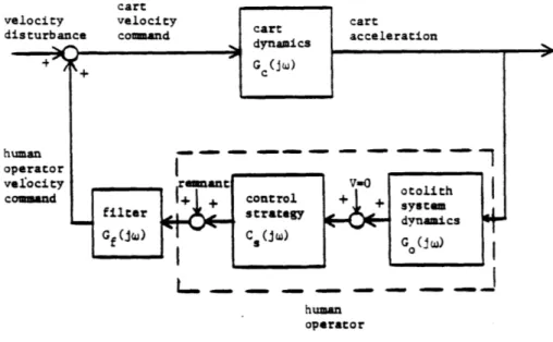
The cart system dynamics have been described in Ref. 12. The model

developed in this reference was found using bond graph techniques and an

assumed cart mass. In order to verify the model, data was taken for a few

runs without HO control. The final test profile was used. One run with no

Subject and one run with a 140 lb. subject were considered. The standard

diata reduction techniques

described in section 3.3 were used with the

velocity

command as the input and the cart acceleration as the output. A

Bode plot of the results is shown in Fig. 3.1.2.01.

This plot shows that the cart transfer

function

can be approximated by a

simple

dilferentiator with a gain

of

1.12. Although there is

some

scatter in the data at the low frequencies it is felt that the more simplified

model for the system is more useful for any further work. This plot and

model were used as required in all further work. It is also seen that the

additional mass of the subject had little effect on the results. This gives

assurances that the analog controller is performing satisfactorily with the

varying

subject mass. It is noted that this model differs from that of Ref.

12.

3.2 Sled System Software

All functions of the Sled are controlled by a single program called CART. Individual functions are accessed from the CART program by two letter

codes. The hierarchy of the CART program is explained in Ref. 13,14 and

will only be described as necessary here. It is noted that the software has

been designed to be "user friendly" and has great flexibility in its

current capability and potential for future growth. All program parameters, which are used extensively in the software descriptions, are denoted by

140 lb. subject no subject

§

0.05 0.10

frequency

(Hz) 0.13 0.20 0.30 0.40 0.50 -

0

mwLU

C

+360 -L.

Figure 3.1.2.01 The Cart Transfer Function Bode Plot

28

0

C

C C z

1.0

0.5 0.0 I'kJ -0. 5 -t--1.5 -2.0 + 0.0

100

+

+200 -+300 I _I

4-%

n

r-I

CM rl

capital

letters.

Safety features have also been incorporated in the cart system software.

checks are made on the commanded velocity to prevent an overvoltage

to the controller.

The cart position and velocity are checked at every

sa.ple to determine if

the cart could reach the track limits.

If

so the

software

decelerates

and stops the cart.

The deceleration

is limited,

however, so often the hardware switches are reached before the cart is

stopped. These are the principle software safety features.

3.2.1 Disturbance Profile Generation

In order to drive the cart with a sum of sinusoids velocity signal two

files have to be created. The first file contains the discrete velocity

commands as determined by the sum of sines. These files are generally

called velocity command profiles,

or profiles,

and their generation is

described in the next section. Each profile is defined by a different set

of parameters. Groups of these profiles are then assigned to files called

protocol files. Each protocol file is made up of a series of profiles. A

profile is run by accessing it from the protocol file using the Sled control panel described in section 3.1. Ref. 13,14 further describe the

file system.

I

All profiles used to run the cart in this work are sum of sinusoids

velocity commands. These profiles are defined by

v(t)

= ZA sin(jInT+p

)

where v(t) is the velocity time history in m/s: A. is the peak amplitude

30

i seconds/sample; n is the consecutive sample number: and t is time = nT.

The program used to generate a sum of sinusoids profile is accessed by

the

SO

command.

Ten parameters are needed to generate a sum of sines

profile. The profile run time, in seconds, is input as variable TRUN.

It is

used to determine the fundamental or base frequency in rad/sec by

b = 2'r/TRUN

The fundamental frequency is also input in Hz. This is used by the test

conductor for illustrative purposes. The number of sinusoids used in the

profile is input as variable NSINES. The disturbance frequencies used in

the profile are determined by the h numbers stored in a data file. Prime

numbers and one even number, if desired, can be used without having the

harmonics of the frequencies affect each other. The disturbance

frequencies are determinei by

W.

_{= h ib}

The FLAT input parameter sets the peak amplitudes at the disturbance

frequencies of either position, velocity, or acceleration constant. For a

constant velocity profile the velocity amplitudes, Ai, are set to

A = 1.0

For a constant position profile the velocity amplitudes are set to

Ai = W

For a constant acceleration profile the velocity amplitudes are set to

A = 1.0/wi

,pitudes before the limit checks are made. This will be discussed in

section

3.2.2.

The frequency variation of each sinusoid is adjusted by the DEL input

phase angle. This is done to give more flexibility and allow each sinusiod

to have a different starting point. The phase angle for each sine is found

by

9

=

i*DEL

i=0,1,....NSINES-1

DEL

is chosen so that no phase angle is duplicated.

With all these

parameters

chosen the sines are completely defined. The amplitudes can now be further adjusted by the input track length limit,

FPOS, in m, and the input acceleration limit, FACC, in g's. The track

length limit is checked first. The sum of sines velocity is integrated to give the position. With the input sampling time, T, the maximum and minimum

position of the run are found using

position(t)

=

Z(Ai/wi)sin(w nT+Pi-7)

If the maximum position excursion exceeds the FPOS limit then the

amnlitudes are scaled by

Ai

=

Ai(FPOS/(posmax

- Posm))

Using these newly defined amplitudes the maximum absolute acceleration, in

g's, is found by

acceleration(t)

=

ZAoW sin(winT+

(9+70)/9.81

If this acceleration exceeds the

FACC

limit the amplitudes are further

32

A = A. (FACC/laccma

I)

At

this point the profile is completely defined. The velocity is then checked to find the

first

zero crossing, at a time to. The phase angles are

then adiusteel so the profile will start at this point. This insures that

the first velocity commanded by the profile is small. The starting position

iq

then calculated by

finding

the position at t0 and then finding

starting position = pos(t₀) - (posmax - posn)/2.0

This centers the profile within the cart travel limits.

This completes the profile generation phase. Two more steps are then used

to store the profile in a data file, and assign this data file to a

protocol file. When these steps are complete the profile can then be used

to run the cart.

The profile generation program has been programmed on two different

computers. Appendix B contains the program listings and a brief

explanation of their use. Only the VAX output calculates the maximum

commanded velocity and the histogram values. The histogram data is found by

calculating each nT acceleration command value using the equation

previously defined. The values of these points are then filed into ranges

of multiples of 0.005 g

ani

counted.

The maximum value of each 0.005 g

range and the number of points in each range is then determined.

3.2.2 Profile Amplitude Scaling

As stated in the previous section the amplitudes of the disturbance

frequencies can be scaled by using the FILTER and FPOLE variables. These

Parameters define the order and pole location of a low pass filter. The

method used to define this scaling will now be developed.

The velocity command is written as

v(t)

=

ZAisin(winT+oi)

When

filtering

is used the amplitudes, Ai, are adjusted so that the power spectral density of the velocity is scaled according to

W.

imax

f

D

v

(w)dw=(K/(

FPOLE+j

w)

FI

LTER) 2

imi n

The amplitudes at each frequency are then chosen to be

imax

1/2A

=

AI

f

DV(V)dw=Ai

( imax)

-

imin)

imin

where

g(w)

is the indefinite integral of f@vv(w)dw

and the

W

imax and Wimin

are chosen to be the geometric means between the disturbance frequencies.

For interior points between disturbance frequencies these frequencies are

found by

Wimax

=

(uiWi+i)

0.5,

and

Wimin

=

(Wjw-1)0.5

The lowest Wimin frequency, w₀ , is found by assuming that the lowest

disturbance frequency,wl, is the geometric mean of the lowest wo and the

next lowest disturbance frequency, w ₂. Thusly , w, can be found by'

W1 = W0 2)0.5

Solving for w then gives

W0 = (12

2

Similarly the highest Wimax Frequency, WNSINES+1, is found by

34

Trhe K value is chosen by specifying the variance of the velocity pijtudes,

fran 0.0, to be 1.0. This gives:

WImax

WNSINESmax

W

NSINESmax

2 = 1.0 = 11/2A 2 f

vv(c)+dw++

04vv()dw - Kf

vv

Mdw

d

O1min

WNSINESmin

1min

so

, NSINESmax

F-1.0/

*1min

vv(w)dw

-

1.0/[g(wNSINES+1-

-Te final equation for the filtered amplitudes can now be written as

Ai

=

Ai

2

SgWNSINES+1)

~

g(WO

The indefinite integrals are readily calculated and will not be elaborated

upon here.

3.2.3 The Digital Joystick Filter

As stated in section 3.1 the joystick signal is filtered before it is

added to the stored velocity cammand. A digital first order low pass filter

is used. The software implementation of this digital filter is

Y(n) - (1-a)Y(n-1)+(a/JSCALE)U(n)

where Y(n)

is

the filtered

output:

U(n)

is the filter

input,

or raw

iovstick signal: and n is the sample number. JSCALE and

a

can be varied by

using the JO command in the CART program. In analog form this filter is

represented by

Y(s) = (K/(1.0/T+s))U(s)

K

=

1.0/JSCALE,

T=

T/ln(1.0-a)

X.5is seen the JSCALE variable is used to vary the gain of the Filter and

the

a variable

is used to vary the pole of the

filter. As is shown in

,haoter 4, JSCALE is an important oarameter in determining the success of a

profile -a

was

set

at

a

=0.1

and

never varied

throughout

the profile

ievel onment.

With a=0.1 the equivalent time constant is

T=0.095

sec. From the

stripcharts

of the cart velocity during full deflection tests of the

joystick it was seen that the cart response had no visible delay and no

overshoot. To increase the time constant would lower this response time

which would he easily noticed by the HO. Also, the human sensory system

operates with a 0.20 sec time constant which gives a sufficient safety

margin compared to

T=0.95

sec.

It would not be desirable to increase

T

as

this would decrease the safety margin and possibly cause resonance effects

similar to pilot induced oscillations. There is no reason to decrease

T,

as the response of the cart is quite acceptable. For these reasons a was

not varied.

3.3 Data Reduction

A data file is created

for

every run during which the data storage flag is enabled. The A/D's used to convert the output signals have 8 channels.

The 5 outputs available for this work are found in channels 1,2,3,4, and 6.

The data points are grouped into blocks of 256 noints which gives 32

samples of each channel per block. The PDP 11/34 minicomputer is used to

To

reduce this data each channel is accessed individually and stored in a

file.

This is done by storing every 3th + desired channel * point of the

original

data File. The data is then concatenated to produce 1024 points to

be

used to run the Fast Fourier Transform (FT) algorithm.

The total number of data points of each output of each run is Found by

run time/sampling rate = TRUN/0.01

The number of

noints for

each concatenation is then found by

N

=

TRUN/(0.01)A1024)

From

the ensemble of N points an average and standard deviation are

<ietermined. Any of the N noints which are more than two standard

deviations

from

the average are discarded and a new average is determined.

The percentage of the discarded points is printed out as REJECT. This new

average is then stored in an array of 1024 points. When all 1024 points are

found the averaqe, AVG, square root of the mean squared error, RMS, and the standard deviation, STD, are calculated.

With the concatenation of all channels comnlete, an FFT is used to find

the 'recuencv distribution. A simple fortran

FFT

proqram obtained from Ref. 1; was coded into the PDP-11/34 minicomputer. This allows the data to be

nrocessed directly

from

the stored data

files

obtained during the test

runs. Two programs are run sequentially to obtain the Final results.

The first

amplitude and phase obtained fram the FFT are the bias values.

The subsecuent values are associated with a frequency, f, defined by

here I is the array position. The I-1 factor is needed since the first

array values are the bias values as stated. The run time, TRUN, is

specified to be a multiple of 1024 times the

sampling rate.

This insures

that the disturbance frequencies can be exactly reproduced

by the FFT.

The

remnant

frequencies

and values are

found by averaging

the amplitudes,

phases, and frequencies of all the points between the disturbance

frequencies. Although this is not precisely correct, the real and imaginary

parts should be averaged and then the amplitude and phase determined, Ref.

8 shows that there is a negligible difference between the two methods of computation. The log(GAIN) and phases of the transfer function are then

determined by

FAMPJ(

N+1)

log(GAIN(N)

)=log

, phase(N)=PHASEJ(N+1)-PHASEA(N+1)+180

AMPA(N+1)

where AMPJ is the joystick amplitude: AMPA is the acceleration amplitude:

PHASEJ is the joystick phase angle: PHASEA is the acceleration phase angle. The 180 deg. correction is added since the subject opposes the cart motion.

All count values are converted to engineering units with the calibrations

of section 3.1 before entering the FFT program. The desired plots are then

created with this data. An explanation of the plots is contained in

Appendix E.

It is noted that the FFT does not correct for the run time used. This

means that the ouput is not scaled in a meaningful way.

This results in the

high amplitude values seen in the frequency spectrum plots. To keep this in

mind when looking at these plots, the designation FFT has been placed in

38

data as the scaling factors are canceled when the amplitude ratios are

ta ken

for

the GAIN

and

phase data.

For runs that are not completed; (i.e.

the subject did not stay within

tie track limits for the full run time) no FFT information

was obtained.

Since it was desired to work with only completed runs for the procedure

little effort was expended on analyzing incomplete runs. A program was

written to calculate the RMS, AVG, and STD values of all data points for a run, however. This was used for the initial testing since most of these

runs were incomplete. The RMS, AVG, and STD values were computed from only the concatenated 1024 points for all further runs. There is a few

precentage points of error between the two methods of computation but it is

not of significance for this work.

Listings of all the programs used to reduce data in this work are

provided in Appendix C. Brief descriptions of their use, along with input

and output samples, are included.

TEST PROCEDURE DEVELOPMENT

4.1 General Concepts

The background of the pre- and post-flight closed-loop otolith system

testing has been developed in Chapters 1 and 2. One key factor of this test

is that it is to be used on all participating astronauts. Therefore, there

could be some variation of otolith sensitivity among the subjects. Also, as

stated in Chapter 1, it is expected that adapting to weightlessness will cause a decrease in otolith sensitivity. This increases the range of

otolith sensitivity at the less sensitive end. Any test procedure must then

have two major goals:

1) yielding an accurate description of the HO response, 2) yielding this description for a wide range of otolith

sensitivities.

As mentioned in Chapter 2 the test period will be of limited duration and data analysis needs to be performed without delay. Because of this it is

felt that the test procedure should offer good chances for completing runs

with little practice. This also means that some margin for error in control

will

be available,

which

should be

helpful

for

subjects with varying

otolith sensitivities. Further, it means that the test is not so difficult

that results might be in question due to short runs. Finally it gives

confidence in the procedure itself.

The data analysis can also be performed in a more straightforward manner

40

problems of FFT analysis with incomplete runs and gives more consistent

reSults.

The run completion rate is therefore of major practical importance

developing a test procedure.

Initially a computer simulation of the closed-loop system was desired to

help determine the general ranges of the system parameters. With the first

testing, however, this idea was abandoned. The effects seen were very

non-linear and so would not have been evident in a non-linear simulation. The main

thrust of the development was then based on experimental results. Lessons

learned

from one set of tests were applied to determine the next profiles.

This was continued until a profile was found that fit the previous

criteria. A description of this development now follows.

4.2 The DHPR02.PRO Series, Part 1, and High Amplitude Problems

As stated previously the authors initial experience with the closed-loop

nulling task was as a subject in the tests of Ref. S. The parameters used to generate this profile are shown in Fig. 4.2.01. This initial experience

suggested that a smaller track length be used to help subjects remain

within the track limits. Also, it was felt that a run time of 184.32 sec.

was too long as in the author's experience fatigue became a factor after

about 120 sec.

Using this experience seven profiles were created. The flat velocity

calculation was used to scale the amplitudes as this lessened the number of

variables required to generate the profiles. The track length was lowered

to a range of 1.97-2.38 m while the corresponding maximum accelerations

41

IN THE SUM AMP CM/SJ 0.08 0.09 0.11 0.11 0.10 0.10 0.10 0.12 0.10 0.09 0.10 0.07 0.06 0.08 0.08 0.08 0.07 0.06 0.05 0.04 0.04 0.02 0.02 0.02 0.02 OF SINUSOIDS: ACCEL AMP CG3 0.001 0.002 0.003 0.004 0.05 0.006 0.006 0.009 0.010 0.010 0.012 0.010 0.010 0.013 0.015 0.018 0.018 0.019 0.019 0.018 0.017 0.013 0.013 0.013 0.012 MAXIMUM ACCELERATION IN SIGNAL: PERCENT USAGE OF TRACK: 100.00%

PHASE CDEGJ 0. 247. 134. 21. 268. 156. 43. 290. 177. 64. 311. 198. 85. 332. 220. 107. 355. 242. 130. 17. 265. 153. 40. 288. 176. 0.140 G STARTING POSITION: 0.00

Figure 4.2.01 Profile Parameters of Ref. 8

I

RESULTING FREO CHZ3 0.016 0.027 0.033 0.060 0.07t 0. 092 0.103 0.125 0.157 0.168 0.201 0.222 0.233 0.255 0.288 0.331 0.396 0.450 0.548 0.613

0.743

0.808 0.884 0.982 1.080

SUM OF SINES PROFILE

1. DURATION OF PROFILE: 184.32 SEC PARAMETERS OF SINUSOIDS:

2.

NUMDER OF

SINUSOIDS:

25 3. FUNDAMENTAL FREQUENCY* 0.0054 HZ

4. EQUAL AMPLITUDE DOMAIN: 0 (-1,P;oV;+1tA)

5.

SUCCESSIVE PHASE ANGLE: 247.

DEG

PARAMETERS OF SHAPING FUNCTION:

6. ORDER OF FILTER: 2

7. POLE: 0.28 HZ

PHYSICAL CONSTRAINTs:

8.

LENGTH OF TRACK 3.60 M

9. ALLOWED ACCELERATION 0.41 G

I

42

FREU. (HZ) 0.0488 0. 107 A 0.It60 0.1855 0. 2246 0.2$37 0.3027 0.3613 0.4004 0 .4 i90 0. 176 AMPi (M/S) 0.13 0.13 ) .13 0.13 0.13 0.13 0.13 0.13 0.13 0.13 0.13 ?MP2 (i) 0 1O 4 0.019 0.019 0 .024 0.02" 0.030 0.033 0.038 0.043 PHASE (DEG) 0. 247. 134. 21. 26. 155. 43. 290. 177. 64. 311.

Figure 4.2.02 DHPRO2.PRO Profile #6 Parameters

INFUI PARAMETERS TRUN- 102.400 NSINESj 11 FFRkU- 0.009766 FLAr : 0 DEL- 247.000 FILTERx 0 FPOLE- 0.310 FFlS-- 3.5t FACCz 0.300 TLOOP 0.010 ROFILE DESCRIPTION MAX ACCEL- 0.:'04 VELMAA- 1.1460 USEAGE U 1-FeCKz t7.50 ST ARrt IG POSITICN=-0.363 SCALE= 0.1881

,ere used to test the eF-cts of these variables. The same DEL=247 was used

to eliminate the effects of varying this value. One of the profiles is

_,,ownin Fig. 4.2.02. Five subjects were tested. The open-faced head

restraint was used and subjects were asked to close their eyes during the

runs. A blindfold was not used.

The results of these tests were most illuminating qualitatively. Very

few runs were completed. The main effects seen were as follows:

1) subjects often lost track of their direction of motion and it was

common to make the initial control in the wrong direction. Often this ended a run. This was probably caused by the vibration of the cart

giving a velocity cue without an acceleration cue during approximate

constant velocity motion.

2)- There was no tendency to end all runs at the same end of the track.

It is noted in Ref. 5 that for angular motion this is not the case.

3) Control was sensitive and HO induced oscillations were not uncommon. Often high frequency oscillations were injected by the subject to

decrease their response time and to attempt to find the zero input

range of the joystick. Also, the high input accelerations at the higher

frequencies probably contributed to the HO induced oscillations.

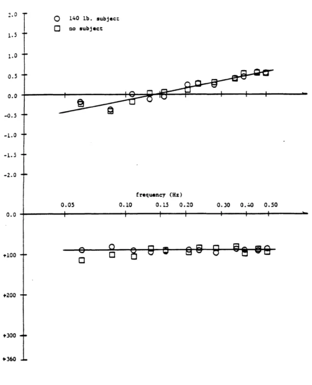
Bode plots were found for each completed run. A typical plot is shown in Fig. 4.2.03. (Appendix E contains a discussion of the plot formats.) The

plot shows the general trends expected by the Young and Meiry model. The

drop in gain with higher frequencies is clear, but the phase remains

relatively flat. There is much data scatter, especially in phase, which signifies a large number of direction reversals. This corresponds with the large amount of HO induced oscillations observed during test runs. This